Gravitational recoil in nonspinning black-hole binaries: The span of test-mass results

Abstract

We consider binary systems of coalescing, nonspinning, black holes of masses $m_{1}$ and $m_{2}$ and show that the gravitational recoil velocity for any mass ratio can be obtained accurately by extrapolating the waveform of the test-mass limit case. The waveform obtained in the limit $m_{1}/m_{2}\ll 1$ via a perturbative approach is extrapolated in $\nu=m_{1}m_{2}/(m_{1}+m_{2})^{2}$ multipole by multipole using the corresponding, analytically known, leading-in-$\nu$ behavior. The final kick velocity computed from this $\nu$-flexed waveform is written as $v(\nu)/c=0.04457\nu^{2}\sqrt{1-4\nu}\,(1-2.07106\nu+3.93472\nu^{2}-4.78404\nu^{3}+2.52040\nu^{4})$ and is compatible with the outcome of numerical relativity simulations

I Introduction

Interference between the multipoles of the gravitational waves (GW) emitted from coalescing black-hole binaries of masses $m_{1}$ and $m_{2}$ carries away linear momentum and thus imparts a recoil to the final merged black hole. The accurate calculation of this recoil velocity, also referred as kick, has been the topic of analytical and numerical studies in recent years Damour and Gopakumar (2006); Sopuerta et al. (2006); Schnittman et al. (2008); Baker et al. (2006); Gonzalez et al. (2007, 2009); Campanelli et al. (2007); Le Tiec et al. (2010); Lousto and Zlochower (2011a); Lousto and Zlochower (2013); Buchman et al. (2012). In particular, after assessing the properties of the kick velocity for nonspinning black-hole binaries, numerical relativity (NR) went on to investigate the effect the black-hole spins have on the final kick. The most interesting and astrophysically relevant result is that high recoil velocities, of about a few thousands of km/s, can be reached for nonaligned spin configurations Lousto and Zlochower (2011a); Lousto and Zlochower (2013).

When one black hole is much more massive than the other, ${\mathsf{M}}\equiv m_{2}\gg{\mathsf{m}}\equiv m_{1}$ (${\mathsf{m}}/{\mathsf{M}}\equiv 1/q\ll 1$), the kick is obtained from the GW emission computed using black hole perturbation theory Bernuzzi and Nagar (2010); Sundararajan et al. (2010). When the larger black hole is nonspinning, Ref. Bernuzzi and Nagar (2010) used Regge-Wheeler-Zerilli (RWZ) perturbation theory Nagar and Rezzolla (2005) to calculate the GW emission from the transition from inspiral to plunge of a point-particle source subject to leading-order (LO) analytical (effective-one-body), resummed radiation reaction force. When the larger black hole is spinning, Sundararajan et al. (2010) solved the Teukolsky equation with a point-particle source term subject to a numerical, adiabatic, radiation reaction force. In the nonspinning case, both studies essentially agreed on the value of the final recoil velocity: Ref. Sundararajan et al. (2010) got $v/[c({\mathsf{m}}/{\mathsf{M}})^{2}]=0.044$, using up to $\ell=6$ multipoles, while Ref. Bernuzzi and Nagar (2010) estimated $v/[c({\mathsf{m}}/{\mathsf{M}})^{2}]=0.0446$ using multipoles up to $\ell=8$. Reference Sundararajan et al. (2010) studied whether the perturbative result can be accurately extrapolated to any mass ratio using the $\nu$-scaling corresponding to the LO multipolar contribution Fitchett and Detweiler (1984)

$$v(\nu)/c=0.044\nu^{2}\sqrt{1-4\nu},$$ (1)

where $\nu=m_{1}m_{2}/M^{2}$, with $M=m_{1}+m_{2}$, is the symmetric mass ratio. It was found that this scaling is rather inaccurate when $\nu\sim 0.2$, as it predicts values that are larger by $\sim 50\%$ than the NR results.

In this paper we show that extrapolating in $\nu$ the test-mass waveform multipole by multipole up to multipole order $\ell=8$ and then computing the recoil from this $\nu$-flexed waveform, allows one to get an improved version of the LO scaling that is compatible with the NR results of Refs. Gonzalez et al. (2007, 2009); Buchman et al. (2012).

II Extrapolating in ${\bm{\nu}}$ test-mass results

Let us start by pointing out a systematic flaw in assuming the LO scaling (1). The RWZ-normalized multipolar decomposition of the waveform is (for equatorial motion)

$$\vspace{-2.5mm}h_{+}-{\rm i}h_{\times}=\dfrac{1}{r}\sum_{\ell=2}^{\ell_{\max}}\sum_{m=-\ell}^{\ell}\sqrt{\dfrac{(\ell+2)!}{(\ell-2)!}}\;{\rm i}^{{\epsilon}}\Psi^{(\epsilon)}_{{\ell m}}{}_{-2}Y^{{\ell m}}(\theta,\phi),$$

where $\epsilon=0,1$ is the parity of $\ell+m$. The functions $\Psi^{(\epsilon)}_{{\ell m}}\equiv\Psi_{{\ell m}}^{(\epsilon)}(t;\nu)$, (e.g., computed from a NR simulation), are normalized as in Ref. Bernuzzi and Nagar (2010). In the perturbative context $(\nu\to 0)$, they are a solution of the Zerilli ($\epsilon=0$) and Regge-Wheeler ($\epsilon=1$) equations with a point-particle source term Nagar et al. (2007); Bernuzzi and Nagar (2010). The GW linear momentum flux in the equatorial plane is

$${\cal F}_{x}^{\bf P}+{\rm i}{\cal F}_{y}^{\bf P}=\dfrac{1}{8\pi}\sum_{\ell=2}^{\ell_{\max}}\sum_{m=-\ell}^{\ell}{\rm i}\bigg{[}a_{{\ell m}}\dot{\Psi}_{\ell m}^{(0)}\dot{\Psi}^{(1)*}_{\ell,m+1}$$

$$+b_{\ell m}\sum_{\epsilon=0,1}\dot{\Psi}^{(\epsilon)}_{\ell m}\dot{\Psi}^{(\epsilon)*}_{\ell+1,m+1}\bigg{]},$$ (2)

where the numerical coefficients $(a_{\ell m},b_{\ell m})>0$ are given in Eqs. (16)-(17) of Bernuzzi and Nagar (2010), and $\Psi^{*}_{{\ell m}}=(-1)^{m}\Psi_{\ell,-m}$. The (complex) recoil velocity at time $t$ is obtained as

$$v_{x}+{\rm i}v_{y}=-\dfrac{1}{M}\int_{-\infty}^{t}\left({\cal F}_{x}^{\bf P}+{\rm i}{\cal F}_{y}^{\bf P}\right)dt^{\prime}.$$ (3)

For each multipole, the leading-in-$\nu$ (completely explicit) dependence is Damour et al. (2009) $\Psi_{\ell m}^{(\epsilon)}\propto\nu c_{\ell+\epsilon}(\nu)$, where $c_{\ell+\epsilon}(\nu)\equiv X_{2}^{\ell+\epsilon-1}+(-)^{m}X_{1}^{\ell+\epsilon-1}$, with $X_{i}=m_{i}/M$ so that $X_{1}+X_{2}=1$ and $X_{1}X_{2}=\nu$. The convention we adopt here is $X_{2}>X_{1}$, i.e., $X_{2}-X_{1}=\sqrt{1-4\nu}$, so that $c_{\ell+\epsilon}(0)=1$. The explicit $\nu$-dependence in Eq. (II) comes as sum of products of $c_{\ell+\epsilon}(\nu)$. Defining individual rescaled fluxes as $\hat{\cal F}_{\ell m\ell^{\prime}m^{\prime}}\equiv{\rm i}/(8\pi)\alpha_{{\ell m}}\dot{\Psi}_{{\ell m}}^{(\epsilon)}\dot{\Psi}_{\ell^{\prime}m^{\prime}}^{(\epsilon^{\prime})*}/[\nu^{2}c_{\ell+\epsilon}(\nu)c_{\ell^{\prime}+\epsilon^{\prime}}(\nu)]$ (with either $\alpha_{{\ell m}}=a_{{\ell m}}$ or $\alpha_{{\ell m}}=b_{{\ell m}}$), Eq. (II) reads

$${\cal F}_{x}^{\bf P}+{\rm i}{\cal F}_{y}^{\bf P}=\nu^{2}\sqrt{1-4\nu}\bigg{\{}\hat{\cal F}_{223-3}+\hat{\cal F}_{2-231}+\hat{\cal F}_{2-221}+\dots$$

$$+(1-3\nu)\hat{\cal F}_{334-4}+\dots+(1-3\nu)(1-2\nu)\hat{\cal F}_{445-5}+\dots\bigg{\}},$$ (4)

where we wrote just a few terms to indicate that the explicit (leading) $\nu$-dependence of the flux is more complicated than just the LO one.

Table 1: Final recoil velocity: comparing the (multipolar) $\nu$-extrapolated RWZ result, $v^{{\rm RWZ}_{\nu}}_{{\rm end}}$, the leading-order extrapolation, Eq. (1), $v^{{\rm RWZ}_{\rm LO}}_{\rm end}$ and the NR values of Buchman et al. (2012). As a conservative error estimate, the $v^{{\rm RWZ}_{\nu}}_{{\rm end}}$ can be larger by 1 to 2$\%$. See text for details.

$q$	$\nu$	$v^{\rm NR}_{\rm end}$[km/s]	$v^{{\rm RWZ}_{\nu}}_{\rm end}$[km/s]	$v^{{\rm RWZ}_{\rm LO}}_{\rm end}$[km/s]
2	$0.\bar{2}$	$148\pm 2$	151.3	219.9
3	$0.1875$	$174\pm 6$	169.5	234.8
4	$0.1600$	$157\pm 2$	154.2	205.2
6	$0.1224$	$118\pm 6$	114.1	143.1

Let us consider now the $\nu\to 0$ gravitational waveform $\Psi_{\ell m}^{(\epsilon)}(t;0)$ obtained solving the RWZ equations with a point-particle source subject to leading-order, resummed, analytical radiation reaction force. The mass ratio is ${\mathsf{m}}/{\mathsf{M}}=10^{-3}$. This waveform was computed in Ref. Bernuzzi et al. (2011) using the hyperboloidal layer approach Zenginoglu (2010), which allowed us to: i) extract waves at ${\mathrsfs{I}}^{+}$; ii) obtain high-resolution data (the numerical error is not an issue). The quasicircular inspiral starts at $r_{0}=7{\mathsf{M}}$. The recoil velocity obtained from Eq. (II) with $\ell_{\max}=7$ is $v(0)/[c({\mathsf{m}}/{\mathsf{M}})^{2}]=0.04457$, consistent with Bernuzzi and Nagar (2010). Analyzing the corresponding $\hat{{\cal F}}_{\ell m\ell^{\prime}m^{\prime}}(t;\,0)$’s ($\nu\equiv{\mathsf{m}}/{\mathsf{M}}$, $c_{\ell+\epsilon}(0)=1$), one finds that the (complex) coefficients of the different $\nu$-dependent terms in the curly bracket of Eq. (II) are essentially in phase. It follows that the $\nu$-extrapolation of $v(0)$ done using Eq. (1) [i.e., ignoring the extra factors $(1-3\nu)$, $(1-3\nu)(1-2\nu)$ etc. in Eq. (II)] is inaccurate (and in particular gives a value larger than the correct one) at least because the $\nu$ dependence of several subleading terms crucially contributing to the momentum flux is not taken into account correctly. For example, for $\nu=0.2$, where the function $\nu^{2}\sqrt{1-4\nu}$ gets its maximum, the values of the extra $\nu$-factors are $(1-3\times 0.2)=0.4$ and $(1-3\times 0.2)(1-2\times 0.2)=0.24$. The LO $\nu$-scaling is then incorrectly amplifying $\hat{{\cal F}}_{334-4}$ and $\hat{{\cal F}}_{445-5}$ by 2.5 and $4$ times respectively.

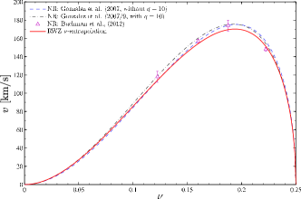
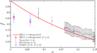
Figure 1: (color online) Top: magnitude of the final recoil velocity versus $\nu$. The data points of Buchman et al. (2012) and the fits to the NR data of Refs. Gonzalez et al. (2007, 2009) are compared with the result of the extrapolation in $\nu$ of the RWZ multipolar waveform (red curve). Bottom: the extrapolated reduced function $\tilde{f}(\nu)\equiv v(\nu)/[v(0)\nu^{2}\sqrt{1-4\nu}]$ contrasted with the actual NR data of Gonzalez et al. (2007, 2009); Lousto et al. (2010); Lousto and Zlochower (2011b); Buchman et al. (2012).

To extrapolate in $\nu$ the multipolar waveform, we take $\hat{\Psi}^{(\epsilon)}_{{\ell m}}(t;\,0)\equiv\Psi^{(\epsilon)}_{{\ell m}}(t;\,0)/({\mathsf{m}}/{\mathsf{M}})$, multiply it by the corresponding leading-order $\nu$ dependence, so to get the $\nu$-dependent function (addressed as RWZ_ν in the following) $\Psi_{{\ell m}}^{(\epsilon)}(t;\,0_{\nu})\equiv\nu c_{\ell+\epsilon}(\nu)\hat{\Psi}^{(\epsilon)}_{{\ell m}}(t;\,0)$. [The notation $0_{\nu}$ is a reminder that only the leading order $\nu$ dependence of each multipole is included and so $\Psi^{(\epsilon)}_{\ell m}(t;\,0_{\nu})\neq\Psi^{(\epsilon)}_{\ell m}(t;\,\nu)$]. Using $\Psi_{\ell m}^{(\epsilon)}(t;\,0_{\nu})$ in Eq. (II) we get the linear momentum flux versus time and then the kick velocity via Eq. (3). Since the waveform starts at time $t_{0}>-\infty$, the boundary condition $Mv_{0}\equiv-\int_{-\infty}^{t_{0}}({\cal F}^{\bf P}_{x}+{\rm i}{\cal F}^{\bf P}_{y})dt$ in Eq. (3) is fixed as the center of the velocity hodograph during the inspiral Bernuzzi and Nagar (2010).

Table 1 compares the final kick velocity $v\equiv|v_{x}+{\rm i}v_{y}|$ obtained from the RWZ_ν waveform with the most recent NR calculations Buchman et al. (2012), using the SpEC Scheel et al. (2009) code, with $q=(2,3,4,6)$ (and retaining only multipoles with $\ell\leq 6$). The extrapolated values are very close to the NR ones, in two cases within their error bars. By contrast, the last column of the table highlights how inaccurate the leading-order scaling is. The uncertainty on the RWZ_ν values has essentially two sources: (i) the fact that ${\mathsf{m}}/{\mathsf{M}}\ll 1$, but always ${\mathsf{m}}/{\mathsf{M}}\neq 0$ and (ii) the effect of multipoles selected by the condition $\ell_{\rm max}>7$. In Table III of Ref. Bernuzzi and Nagar (2010) it was shown that changing ${\mathsf{m}}/{\mathsf{M}}=10^{-3}$ to ${\mathsf{m}}/{\mathsf{M}}=10^{-4}$ was increasing the final kick by $\sim 0.5\%$. In addition, we checked that the relative difference between taking $\ell_{\rm max}=6$ $[v(0)({\mathsf{M}}/{\mathsf{m}})^{2}=0.04383]$ and $\ell_{\rm max}=7$ ($v(0)({\mathsf{M}}/{\mathsf{m}})^{2}=0.04457$) is as large as $\sim 1.7\%$ when ${\mathsf{m}}/{\mathsf{M}}=10^{-3}$, but becomes as small as $10^{-3}$ for $q=6$ and $10^{-4}$ for $q=2$. As a conservative error estimate, the extrapolated values of Table 1 can be larger by $1$ to $2\%$.

Figure 1 compares $v(\nu)$ with $0\leq\nu\leq 0.25$ (solid curve, red online) with available fits obtained from the comprehensive numerical study of Refs. Gonzalez et al. (2007, 2009). We also show the data of Ref. Buchman et al. (2012). The data of Refs. Gonzalez et al. (2007, 2009) are represented by two different fits: $v^{\rm NR}=1.20\times 10^{4}\nu\sqrt{1-4\nu}(1-0.93\nu)$ (dashed, blue online), proposed in Ref. Gonzalez et al. (2007) without including the $q=10$ data of Gonzalez et al. (2009), and $v^{\rm NR}/c=0.04396\nu^{2}\sqrt{1-4\nu}(1-1.3012\nu)$, with $c=299792.458$ km/s (dot-dashed) done in Bernuzzi and Nagar (2010) including the $q=10$ data. The maximum value of the RWZ_ν curve is $v_{\rm max}=170.164$ km/s (at $\nu=0.194$), quite close to $v_{\max}^{\rm NR}=175.2\pm 11$ km/s computed in Gonzalez et al. (2007). A more precise quantitative information is given by (bottom panel of Fig. 1) the normalized quantity $\tilde{f}=v(\nu)/[v(0)\nu^{2}\sqrt{1-4\nu}]$ obtained from the extrapolated $v(\nu)$ (solid line). For completeness, we also exhibit the raw NR data of Refs. Gonzalez et al. (2007, 2009); Buchman et al. (2012) as well as those of Refs. Lousto et al. (2010); Lousto and Zlochower (2011b) for the challenging values $q=15$ and $q=100$, the highest simulated so far. Note that for these $q$’s the recoil velocity is systematically underestimated since the multipoles with $\ell>4$ were neglected in Refs. Lousto et al. (2010); Lousto and Zlochower (2011b). Notably, if the extrapolation is done retaining only the multipoles with $\ell\leq 4$, the RWZ_ν result for $q=15$ and $q=100$ (red circles in the bottom panel of Fig. 1) is compatible with the NR points. The complete RWZ_ν $\tilde{f}(\nu)$ curve is accurately fitted ($\Delta\tilde{f}\equiv\tilde{f}-\tilde{f}^{\rm RWZ_{\nu}}\sim 10^{-5}$) by the quartic trend $\tilde{f}(\nu)=1-2.07106\nu+3.93472\nu^{2}-4.78404\nu^{3}+2.52040\nu^{4}$. [A cubic trend yields instead $\tilde{f}(\nu)=1-2.06407\nu+3.76663\nu^{2}-3.60498\nu^{3}$ with $\Delta\tilde{f}\sim 10^{-4}$, undistinguishable on the scale of Fig. 1. Note that the (less accurate) quadratic trend was instead suggested in both Ref. Damour and Gopakumar (2006) using the effective-one-body formalism and Ref. Sopuerta et al. (2006) using the close-limit approximation]. It would be interesting to extract $\tilde{f}(\nu)$ accurately from ad hoc NR simulations.

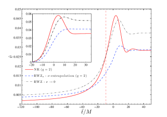
Figure 2: (color online) Time evolution of $\hat{v}\equiv v/(c\nu^{2}\sqrt{1-4\nu})$ for $q=2$ obtained from (a restricted sample of) multipoles of the NR waveform and from the $\nu$-extrapolated RWZ_ν ones. The vertical line indicates the NR merger. Inset: corresponding analytical approximations, Eq. (5), to $\hat{v}(t)$. The nonextrapolated $\nu\to 0$ curves are also shown for completeness.

Table 2: Final and maximal recoil velocity computed from the NR (boldface) and RWZ_ν $\nu$-extrapolated waveform for a restricted sample of waveform multipoles ($\ell,m)$ with $m=\ell$ up to $\ell=6$, (2,1) and (3,2). Here it is $\hat{v}\equiv v/(c\nu^{2}\sqrt{1-4\nu})$.

$q$	$v_{\rm end}$[km/s]	$\max(v)$[km/s]	$\hat{v}_{\rm end}$	$\max(\hat{v})$	$\Delta\hat{v}$
2	139.60	229.94	0.0283	0.0466	0.0183
	141.32	151.72	0.0286	0.0307	0.0029
3	162.04	243.74	0.0308	0.0462	0.0154
	156.70	170.58	0.0297	0.0324	0.0026
4	147.80	210.04	0.0321	0.0456	0.0135
	141.20	155.49	0.0307	0.0338	0.0031
6	107.80	144.17	0.0336	0.0449	0.0113
	102.82	115.12	0.0320	0.0358	0.0038
$\infty$	…	…	0.0374	0.0443	0.0070

Time evolution of kick velocity. – We investigate now if the $\nu$-extrapolation is able to reproduce the structure of the well-known (post-merger) local maximum of $v(t)$, predicted and analytically explained in Damour and Gopakumar (2006) (see also Price et al. (2011)) and now known as “antikick” Schnittman et al. (2008); Rezzolla et al. (2010). Since this information is not given in Buchman et al. (2012), we have to compute $v^{\rm NR}(t)$ from the (limited) number of NR $(\ell,m)$ waveform multipoles of Buchman et al. (2012) to which we have access. For both NR and RWZ_ν we use $\Psi_{{\ell m}}^{(\epsilon)}$ with $m=\ell$ up to $\ell=6$ plus (2,1) and (3,2). Table 2 lists the final and maximum velocity obtained from NR (boldface) and RWZ_ν data (cf. with Table 1), together with the magnitude of the antikick, $\Delta\hat{v}\equiv\max(\hat{v})-\hat{v}_{\rm end}$, with $\hat{v}\equiv v(t)/(c\nu^{2}\sqrt{1-4\nu})$. Even with a limited number of multipoles, the $\nu$-extrapolated $v_{\rm end}$ is accurate; by contrast, the extrapolated antikick is much smaller than the corresponding NR one. The table is complemented by the main panel of Fig. 2, where we contrast the $q=2$ $\hat{v}(t)$ for both NR and RWZ_ν data (the original $\nu\to 0$ curve is also added for completeness). Note that $\hat{v}(t)$ is plotted versus $\bar{t}\equiv t-t_{\rm max}$, where $t_{\rm max}$ corresponds to the maximum of ${\cal F}_{\bf P}\equiv|{\cal F}_{x}^{\bf P}+{\rm i}{\cal F}_{y}^{\bf P}|$. The vertical line indicates the NR merger, defined as the peak of $|\Psi_{22}|$.

Table 3: Characterization of $\max({\cal F}_{\bf P})$ for the NR (boldface) and RWZ_ν waveforms (with a restricted sample of dominant multipoles). Here is $\tilde{\bf{\cal F}}_{\bf P}^{\rm max}\equiv{\cal F}_{\bf p}^{\rm max}/\nu^{2}\times 10^{3}$. The analytical estimate $v^{\rm end}_{A}$ of the final recoil velocity (last two columns) is obtained from Eq. (6).

$q$	$\tilde{{\cal F}}_{\bf p}^{\rm max}$	$\tau_{\rm max}$	$Q$	$\epsilon_{\rm max}$	$v^{\rm end}_{\rm A}[{\rm km/s}]$	$\hat{v}^{\rm end}_{\rm A}$
2	${\bf 3.009}$	7.505	1.770	0.011	174.85	0.0354
	$1.463$	7.780	1.298	-0.486	202.57	0.0410
3	${\bf 4.22}$	7.485	1.666	-0.028	208.47	0.0396
	$2.330$	7.823	1.319	-0.465	224.30	0.0426
4	${\bf 4.816}$	7.526	1.607	-0.065	192.39	0.0418
	$2.930$	7.858	1.335	-0.447	201.621	0.0438
6	${\bf 5.347}$	7.689	1.552	-0.136	141.29	0.0440
	$3.730$	7.905	1.356	-0.422	146.07	0.0455
$\infty$	$6.499$	8.043	1.418	-0.330	…	0.0516

III Discussion

The results presented so far are consistent with the analytical explanation of the structure of the gravitational recoil given in Ref. Damour and Gopakumar (2006). Essentially, Ref. Damour and Gopakumar (2006) argued that the properties of $v(t)$ after the maximum of ${\cal F}_{\bf P}$ are approximately determined by what happens close to the peak of ${\bf{\cal F}}_{\bf P}$. At time $t$ we have the complex integral (3), i.e. $v_{x}+{\rm i}v_{y}={\rm i}{\cal I}={\rm i}\int_{-\infty}^{t}{\cal F}_{\bf P}(t)e^{i\varphi(t)}dt$. Due to the nonadiabatic character of the evolution of the momentum flux, this integral is dominated by what happens near $\max[{\cal F}_{\bf P}(t)]$. Expanding around $t_{\max}$ one gets Damour and Gopakumar (2006)

$$v_{x}+{\rm i}v_{y}\simeq{\rm i}{\cal F}_{\bf P}^{\rm max}e^{{\rm i}\varphi_{\max}}\sqrt{\dfrac{\pi}{2\alpha}}e^{\beta^{2}/(2\alpha)}{\rm erfc}(z),$$ (5)

with $z=-\sqrt{\alpha/2}(\bar{t}-\beta/\alpha)$, where $\alpha\equiv 1/\tau_{\rm max}^{2}(1-{\rm i}\epsilon_{\rm max})$ and $\beta={\rm i}Q/\tau_{\rm max}$. Here $\tau^{2}_{\rm max}\equiv-{\cal F}_{\bf P}^{\rm max}/(d^{2}{\cal F}_{\bf P}/d\tau^{2})^{\rm max}$ is the characteristic time scale associated to the “resonance peak” of ${\cal F}_{\bf P}$; $Q\equiv\omega_{\rm max}\tau_{\max}$, where $\omega\equiv\dot{\varphi}$ can be interpreted as the “quality factor” associated to the same peak, and $\epsilon_{\rm max}\equiv\dot{\omega}_{\rm max}\tau^{2}_{\rm max}$. When $\bar{t}\gg\tau_{\rm max}$, the integrated recoil is analytically expected to be Damour and Gopakumar (2006)

$$v^{\rm end}_{\rm A}\simeq\sqrt{2\pi}{\cal F}_{\bf P}^{\rm max}\dfrac{\tau_{\rm max}}{(1+\epsilon^{2}_{\rm max})^{1/4}}e^{-Q^{2}/[2(1+\epsilon^{2}_{\rm max})]}.$$ (6)

All relevant information to numerically evaluate Eqs. (5)-(6) for NR (boldface) and RWZ_ν data is listed in Table 3. Several observations can be made. First, the presence of the antikick is qualitatively explained by the behavior of the complementary error function ${\rm erfc}(z)$, Eq. (5), when $z$ is complex. Since $\epsilon_{\rm max}$ is small, one sees that $\Im(z)$ is essentially given by $Q$ Damour and Gopakumar (2006). When $Q>0$ the usual, monotonic, behavior of $\rm{erfc}(z)$ is modified so that a local peak (the antikick) appears (see inset of Fig. 2). In particular, when $Q$ is small one finds small or negligible antikicks; when $Q$ is larger the antikicks are larger. Second, looking at the values of Table 3 one sees that, from the quantitative point of view the analytical result leads to estimates of $v^{\rm end}_{\rm A}$ that are always systematically larger than the exact one, from $\sim 25\%$ ($q=2$) to $\sim 38\%$ ($q=\infty$). Third, focusing on the RWZ_ν data, from Table 3 one sees that the values of $\tau_{\rm max}$ and $Q$ do not vary much with the extrapolation with respect to the test-mass ones, contrary to ${\cal F}_{\bf P}^{\rm max}$, which is then the main responsible of getting $\hat{v}^{\rm end}_{\rm A}$ smaller than in the $\nu\to 0$ case. This gives a qualitative, analytical, consistency check of Table 1 and Fig. 1. In addition, from Table 3 one sees that $Q$ is always larger in the NR case than in the RWZ_ν one, which explains qualitatively Table 2. The reason for this is that the extrapolation acts only on the waveform modulus, and not on its phase (and frequency). As $Q=\omega_{\rm max}\tau_{\rm max}$, in the RWZ_ν case $\omega_{\rm max}$ is still driven by the underlying, less bound, dynamics of a particle on Schwarzschild spacetime, which, during late plunge and merger, spans frequencies that are smaller than the corresponding (more bound) NR ones. Similarly one explains the dependence of $\Delta\hat{v}$ on $q$.

IV Conclusions

In the context of coalescing, nonspinning, black-hole binaries, we have found a simple way to correct the leading-order $\nu$-extrapolation of the recoil velocity in the test-mass limit, Eq. (1) (obtained via a perturbative approach) that is fully compatible with state-of-the-art numerical relativity simulations. Our approach is based on extrapolating in $\nu$ the test-mass waveform multipole by multipole using the corresponding leading-in-$\nu$ behavior before computing the recoil. An analogous $\nu$-extrapolation to get the final recoil velocity can be applied to the the waveform generated by a (spinning) particle plunging on a Kerr black hole. In this case, the subtlety is to separately extrapolate in $\nu$ the spin-dependent and the spin-independent part of the waveform because of their different, leading-order, $\nu$-dependence. The accuracy of the procedure will be discussed in future work.

References

- Damour and Gopakumar (2006) T. Damour and A. Gopakumar, Phys. Rev. D73, 124006 (2006).
- Sopuerta et al. (2006) C. F. Sopuerta et al., Phys.Rev. D74, 124010 (2006).
- Schnittman et al. (2008) J. D. Schnittman et al., Phys.Rev. D77, 044031 (2008).
- Baker et al. (2006) J. G. Baker et al., Astrophys.J. 653, L93 (2006).
- Gonzalez et al. (2007) J. A. Gonzalez et al., Phys. Rev. Lett. 98, 091101 (2007).
- Gonzalez et al. (2009) J. A. Gonzalez et al., Phys. Rev. D79, 124006 (2009).
- Campanelli et al. (2007) M. Campanelli et al., Phys.Rev.Lett. 98, 231102 (2007).
- Le Tiec et al. (2010) A. Le Tiec et al., Class.Quant.Grav. 27, 012001 (2010).
- Lousto and Zlochower (2011a) C. O. Lousto and Y. Zlochower, Phys.Rev.Lett. 107, 231102 (2011a).
- Lousto and Zlochower (2013) C. O. Lousto and Y. Zlochower, Phys.Rev. D87, 084027 (2013).
- Buchman et al. (2012) L. T. Buchman et al., Phys.Rev. D86, 084033 (2012).
- Bernuzzi and Nagar (2010) S. Bernuzzi and A. Nagar, Phys. Rev. D81, 084056 (2010).
- Sundararajan et al. (2010) P. A. Sundararajan et al., Phys.Rev. D81, 104009 (2010).
- Nagar and Rezzolla (2005) A. Nagar and L. Rezzolla, Class.Quant.Grav. 22, R167 (2005).
- Fitchett and Detweiler (1984) M. Fitchett and S. L. Detweiler, Mon.Not.Roy.Astron.Soc. 211, 933 (1984).
- Nagar et al. (2007) A. Nagar et al., Class. Quant. Grav. 24, S109 (2007).
- Damour et al. (2009) T. Damour, B. R. Iyer, and A. Nagar, Phys. Rev. D79, 064004 (2009).
- Bernuzzi et al. (2011) S. Bernuzzi et al., Phys.Rev. D84, 084026 (2011).
- Zenginoglu (2010) A. Zenginoglu, Class. Quant. Grav. 27, 045015 (2010).
- Lousto et al. (2010) C. O. Lousto et al., Phys.Rev. D82, 104057 (2010).
- Lousto and Zlochower (2011b) C. O. Lousto and Y. Zlochower, Phys.Rev.Lett. 106, 041101 (2011b).
- Scheel et al. (2009) M. A. Scheel et al., Phys. Rev. D79, 024003 (2009).
- Price et al. (2011) R. H. Price et al., Phys.Rev. D83, 124002 (2011).
- Rezzolla et al. (2010) L. Rezzolla et al., Phys.Rev.Lett. 104, 221101 (2010).