Actuation, propagation, and detection of transverse magnetoelastic waves in ferromagnets

Abstract

We study propagation of ultrasonic waves through a ferromagnetic medium with special attention to the boundary conditions at the interface with an ultrasonic actuator. In analogy to charge and spin transport in conductors, we formulate the energy transport through the system as a scattering problem. We find that the magneto-elastic coupling leads to a non-vanishing magnetic (elastic) energy accompanying the acoustic (spin) waves with a resonantly enhanced effect around the anti-crossing in the dispersion relations. We demonstrate the physics of excitatinig of magnetization dynamics via acoustic waves injected around the ferromagnetic resonance frequency.

1 Introduction

While the exchange interaction is the largest energy scale of ferromagnets, explaining Curie temperatures of up to 1000 K, the static equilibrium and dynamic properties of the magnetization field in ferromagnetic materials are governed by the dipolar and crystal anisotropy fields [1]. Since the total angular momentum of an isolated system is conserved, any change of the magnetization exerts a torque on the underlying lattice, as measured by Einstein and de Haas [2]. Vice versa, a rotating lattice can magnetize a demagnetized ferromagnet [3]. The coupled equations of motion of lattice and magnetization fields have been treated in a seminal paper reported by Kittel [4]. The magnetoelastic coupling parameters are material constants well known for many ferromagnets [5].

Interest in magnetoelastic coupling has recently been revived in the context of the “spin mechanics” concept covered by the present special issue [Editorial SSC]. Here we are interested in the magnetization dynamics acoustically induced by injecting ultrasound into ferromagnets by piezoelectric actuators as bulk [6] or surface [7] plane acoustic waves. The magnetization dynamics in these experiments is conveniently detected by spin pumping [8] into a normal metal that generates a voltage signal via the inverse spin Hall effect [9].

Some of the consequences of magnetoelastic coupling have already been investigated theoretically [4, 10, 11] and experimentally [12, 13] in the literature. While the coupled magnetoelastic dynamics has been well understood decades ago [4, 10, 14], much less attention has been devoted to the interfaces that are essential in order to understand modern experiments on nanostructures and ultrathin films. The Landauer$-$Büttiker electron transport formalism based on scattering theory is well suited to handle these issues thereby helping to understand many problems in mesoscopic quantum transport and spintronics [15, 16]. Here we formulate scattering theory of lattice and magnetization waves in ferromagnets with significant magnetoelastic coupling. Rather than attempting to describe concrete experiments, we wish to illustrate here the usefulness of this formalism for angular momentum and energy transport.

We consider magnetization dynamics actuated by ultrasound for the simplest possible configuration in which the magnetization direction is parallel to the wave vector of sound with transverse polarization (shear waves). The corresponding bulk propagation of magnetoelastic waves was treated long ago by Kittel [4] who demonstrated that the axial symmetry reduces the problem to a quadratic equation. The injected acoustic energy is partially transformed into magnetic energy by the magnetoelastic coupling that can be detected by spin pumping into a thin Pt layer. For this symmetric configuration and to leading order a purely AC voltage is induced by the inverse spin Hall effect (ISHE) [17] that might be easier to observe by acoustically induced rather than rf radiation induced spin pumping, since in the former the Pt layer is not directly subjected to electromagnetic radiation. The configuration considered by Uchida et al. [6], in which pressure waves generate a DC ISHE voltage by a magnetization parallel to the interfaces, will be discussed elsewhere.

2 Kittel’s equations

We consider a ferromagnet with magnetization texture $\mathbf{M}\left(\mathbf{r},t\right)$ with constant saturation magnetization $\left|\mathbf{M}\right|=M_{0}$. In the following we consider small fluctuations around the equilibrium magnetization $M_{0}\mathbf{z.}$ The classical Hamiltonian can be written as the sum of different energies

$$\mathcal{H=H}_{Z}+\mathcal{H}_{ex}+\mathcal{H}_{me}+\mathcal{H}_{p}$$ (1)

The magnetic Zeeman energy reads

$$\mathcal{H}_{Z}=\frac{\omega_{0}}{2\gamma M_{0}}\left(M_{x}^{2}+M_{y}^{2}\right)$$ (2)

where $\gamma=\left|\gamma\right|$ is the gyromagnetic ratio, $\omega_{0}=\mu_{0}\gamma H$ is the magnetic resonance frequency for an effective magnetic field $H\mathbf{z}$ and $\mu_{0}$ the permeability of free space. The exchange energy cost of the fluctuations

$$\mathcal{H}_{ex}=\frac{A}{M_{0}^{2}}\left[\left(\nabla M_{x}\right)^{2}+\left(\nabla M_{y}\right)^{2}\right]$$ (3)

where $A$ is the exchange constant. The magnetoelastic energy for cubic crystals and magnetization in the $z$-direction can be parameterized by the magnetoelastic coupling constant $b_{2}:$

$$\mathcal{H}_{me}=\frac{b_{2}}{M_{0}}\left(M_{x}\frac{\partial R_{x}}{\partial z}+M_{y}\frac{\partial R_{y}}{\partial z}\right)$$ (4)

where $\mathbf{R}=\left(R_{x},R_{y},0\right)$ is the displacement vector of a transverse lattice wave propagating in the $z$-direction. $\mathcal{H}_{me}$ can be interpreted as a Zeeman energy associated with a dynamic transverse magnetic field $b_{2}\partial_{z}\mathbf{R}$. The corresponding elastic energy reads

$$\mathcal{H}_{p}=\frac{\rho}{2}\mathbf{\dot{R}}^{2}+\frac{\alpha}{2}\left[\left(\frac{\partial R_{x}}{\partial z}\right)^{2}+\left(\frac{\partial R_{y}}{\partial z}\right)^{2}\right]$$ (5)

in terms of the mass density $\rho$ and shear elastic constant $\alpha.$

The total Hamiltonian $\mathcal{H}$ defines the equations of motion of the coupled $\mathbf{R}$ and $\mathbf{M}$ fields. The results in momentum and frequency space $X\left(t\right)=x\left(k,\omega\right)e^{i\left(kx-\omega t\right)}$ can be simplified by introducing circularly polarized phonon and magnon waves $m^{\pm}=m_{x}+i\sigma m_{y}$, $r^{\pm}=r_{x}+i\sigma r_{y}$ $\left(\sigma=\pm 1\right)$, leading to [4]

$$\left(\begin{array}[c]{cc}i(\omega-\sigma\omega_{m})&\sigma\gamma b_{2}k\\ i\frac{b_{2}k}{M_{0}}&\omega^{2}\rho-k^{2}\alpha\end{array}\right)\left(\begin{array}[c]{c}m^{\sigma}\\ r^{\sigma}\end{array}\right)=0$$ (6)

where $\omega_{m}=\omega_{0}+Dk^{2}$ and $D=2A\gamma/M_{0}$ is the spin wave stiffness. This secular equation is quadratic in $k^{2}$ with 4 roots $\left(s=\pm 1\right):$

$$(k_{s}^{\sigma})^{2}=\frac{\rho\omega^{2}}{2\alpha}-\frac{\omega_{0}-\sigma\omega}{2D}+\frac{\gamma b_{2}^{2}}{2\alpha M_{0}}+s\sqrt{\Delta^{\sigma}}$$ (7)

with discriminants

$$\Delta^{\sigma}=\left(\frac{\rho\omega^{2}}{2\alpha}-\frac{\omega_{0}-\sigma\omega}{2D}+\frac{\gamma b_{2}^{2}}{2\alpha DM_{0}}\right)^{2}+\frac{\omega^{2}\rho}{\alpha D}\left(\omega_{0}-\sigma\omega\right).$$ (8)

The corresponding eigenstates are given by the spinor

$$\psi_{s}^{\sigma}\left(\omega\right)=\left(\begin{array}[c]{c}m_{s}^{\sigma}\\ r_{s}^{\sigma}\end{array}\right)=N_{s}^{\sigma}\left(\begin{array}[c]{c}M_{0}\\ ib_{2}k_{s}^{\sigma}/\left(\omega^{2}\rho-\left(k_{s}^{\sigma}\right)^{2}\alpha\right)\end{array}\right),$$ (9)

where $N_{s}^{\pm}$ is a dimensionless normalization factor.

The dispersion is plotted in Fig. 1 for the parameters appropriate for Yttrium Iron Garnet (YIG): $M_{0}=1.4\times 10^{5}\,\mathrm{A/m},$ $b_{2}=5.5\times 10^{5}\,\mathrm{J/m^{3}},$ $H=8\times 10^{4}\,\mathrm{A/m},$ $D=8.2\times 10^{-6}\,\mathrm{m^{2}/s},$ $\gamma=2.8\times 10^{10}\,\mathrm{Hz\,T}^{-1},$ $\rho=5170\,\mathrm{kg/m^{3}},\,\alpha=7.4\times 10^{10}\,\mathrm{Pa}$ [18, 19, 20] and $\mu_{0}=4\pi\times 10^{-7}\mathrm{NA}^{-2}$. In Fig. 1(a) we plot the solutions for waves rotating with the magnetization that appear to be completely phonon (small dispersion) or magnon like (large dispersion). The latter are evanescent ($k^{2}<0$) below the spin wave gap $\omega_{0}.$ The low-frequency anticrossing is better seen in Fig. 1(c) in which the momentum is plotted on an expanded scale. Spin waves precessing against the magnetization, $\sigma=-1,$ are always evanescent and there is no (anti)crossing with the propagating phonons. When the magnetoelastic coupling is switched off $\left(b_{2}\rightarrow 0\right)$ and $\alpha>4\rho D\omega_{0}$ the pure lattice wave $\omega_{p}=\sqrt{\alpha/\rho}k$ and spin wave $\omega_{m}=\omega_{0}+Dk^{2}$ dispersions may cross twice

$$\omega_{c}=\frac{\alpha}{2\rho D}\left(1\pm\sqrt{1-\frac{4\rho D\omega_{0}}{\alpha}}\right)$$ (10)

$$\overset{4\rho D\omega_{0}\ll\alpha}{=}\left\{\begin{array}[c]{c}\omega_{0}\\ \frac{\alpha}{\rho D}\end{array}=\begin{array}[c]{c}2.8\,\mathrm{GHz}\\ 1.7\,\mathrm{THz}\end{array}\right.$$ (15)

where in the second step we take the limit of small $D$. Around these degeneracy points, of which only the low frequency one is relevant here, the effects of the magnon$-$phonon coupling are most pronounced. In the zero frequency limit the solution with $(k_{s}^{\sigma})^{2}\rightarrow 0$ represents a phonon mode with zero wave number. $(k_{s}^{\sigma})^{\pm}=\gamma b_{2}^{2}/\left(\alpha M_{0}\right)-\omega_{0}/D$ is a purely evanescent magnon for small $b_{2}\$that in principle may become a real excitation when the coupling of the lattice is strong enough to overcome the spin wave gap.

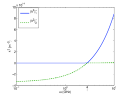
(a)

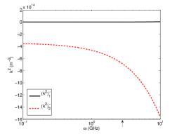
(b)

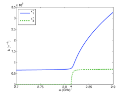
(c)

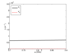
(d)

Figure 1: Dispersion relations of magnetoelastic waves in Yttrium Iron Garnets according to Eq. (7). (c-d) [(a-b)] depict the [squared] momenta of the eigenstates for polarization along and against the magnetic order parameter as a function of frequency. Imaginary momenta appear on the abscissa corresponding to zero real part. The FMR resonance frequency $\omega_{0}$ is indicated by the arrow on the abscissa.

3 Energy flux

Energy conservation implies $\mathbf{\nabla}\cdot\vec{F}=-\partial\mathcal{H}/\partial t,$ where the energy flux $\vec{F}=F\mathbf{\hat{z}}$ consists of phonon and magnon contributions. In time and position space [21]

$$F\left(z,t\right) =-\int dz\frac{\partial\mathcal{H}}{\partial t}=-\frac{2A}{M_{0}^{2}}\frac{\partial M_{x}}{\partial z}\frac{\partial M_{x}}{\partial t}$$

$$-\left(\alpha\frac{\partial R_{x}}{\partial z}+\frac{b_{2}}{M_{0}}M_{x}\right)\frac{\partial R_{x}}{\partial t}+\left(x\longleftrightarrow y\right).$$ (16)

For a plane wave oscillating with frequency $\omega$

$$X\left(z,t\right) =x\left(z,\omega\right)e^{-i\omega t}+x^{\ast}\left(z,\omega\right)e^{i\omega t}$$ (17)

$$=x\left(\omega\right)e^{i\left(kx-\omega t\right)}+x^{\ast}\left(\omega\right)e^{-i\left(kx-\omega t\right)}$$ (18)

the time-averaged energy flux reads

$$\bar{F}\left(z\right)_{x}=-2\omega\operatorname{Im}\left[\frac{D}{\gamma M_{0}}m_{x}\partial_{z}m_{x}^{\ast}+\alpha r_{x}\partial_{z}r_{x}^{\ast}+\frac{b_{2}}{M_{0}}r_{x}m_{x}^{\ast}\right].$$ (19)

In the absence of magnetoelastic coupling, pure phonon and magnon waves

$$\psi_{s}^{\left(m\right)} =N_{s}^{\left(m\right)}M_{0}\left(\begin{array}[c]{c}1\\ 0\end{array}\right)e^{i\left(k_{s}z-\omega t\right)}$$ (22)

$$\psi_{0}^{\left(p\right)} =N_{p}\left(\begin{array}[c]{c}0\\ k^{-1}\end{array}\right)e^{i\left(kz-\omega t\right)}$$ (25)

carry, respectively, the energy fluxes $\bar{F}^{\left(p\right)}$ and $\bar{F}_{s}^{\left(m\right)}:$

$$\bar{F}^{\left(p\right)}=N_{p}^{2}2\alpha\omega/k=N_{p}^{2}2\alpha\sqrt{\alpha/\rho}\,$$ (26)

$$\bar{F}_{s}^{\left(m\right)}=\left(N_{s}^{\left(m\right)}\right)^{2}\frac{2DM_{0}}{\gamma}\omega k_{s}$$ (27)

$$=\left(N_{s}^{\left(m\right)}\right)^{2}\left\{\begin{array}[c]{c}\frac{2D}{\gamma M_{0}}\omega\sqrt{\left|s\omega-\omega_{0}\right|/D}\\ 0\end{array}\,\text{for }\begin{array}[c]{c}s\omega>\omega_{0}\\ s\omega<\omega_{0}\end{array}\right..$$ (32)

One of the magnon states is always evanescent, while the other becomes propagating for frequencies above the magnon gap $\omega_{0}.$ It is then convenient to define

$$\left(N_{p}\right)^{2}=\frac{1}{2\alpha\sqrt{\alpha\rho}};\;\left(N_{s}^{\left(m\right)}\right)^{2}=\frac{\gamma}{2\omega M_{0}}\frac{\Theta\left(s\omega-\omega_{0}\right)}{\sqrt{D\left|s\omega-\omega_{0}\right|}}.$$ (33)

such that each state carries a unit of flux. The flux carried by propagating $\left(\operatorname{Im}k_{s}^{\sigma}=0\right)$ mixed states reads

$$\bar{F}_{s}^{\sigma} =2\omega k_{s}^{\sigma}\left(N_{s}^{\sigma}\right)^{2}\left[\alpha\left(\frac{b_{2}k_{s}^{\pm}}{\omega^{2}\rho-\left(k_{s}^{\pm}\right)^{2}\alpha}\right)^{2}\right.$$

$$\left.-\frac{b_{2}^{2}}{\omega^{2}\rho-\left(k_{s}^{\pm}\right)^{2}\alpha}+\frac{DM_{0}}{\gamma}\right].$$ (34)

while the time-averaged flux for evanescent waves with $\operatorname{Im}k_{s}^{\sigma}\neq 0$ and $\operatorname{Re}k_{s}^{\sigma}=0$ can be shown to vanish identically. By setting $\bar{F}_{s}^{\sigma}$ to unit flux in Eq. (34) we define the dimensionless flux normalization factor $N_{s}^{\sigma}$ for the mixed state. Here and in the following $\sigma$ is the chirality and $s$ the root of an eigenstate. Note that this normalization is rather arbitrary. We could have also used angular momentum flux normalization, or fix the amplitude of one component to unity. We believe, however, that for more general situations with reduced symmetry and many wave vectors, the present choice is most convenient.

4 Interface boundary conditions

We consider a weakly damped ferromagnetic structure actuated by a piezoelectric layer (Fig. 2) that is excited at a given resonance frequency $\omega.$ We assume that any reflection vanishes at the end of the ferromagnet, e.g. by attaching an acoustic absorber [6]. Both actuator and ferromagnet are thus considered to be reservoirs adiabatically connected to the scattering region. In and outgoing waves are then all propagating. We then may disregard negative wave numbers in the ferromagnet as well as the scattering coefficients $\mathfrak{r}^{\prime}$ and $\mathfrak{t}^{\prime}$, the reflection and transmission coefficients of waves from the magnetic side. On the left side we have incoming circularly polarized phonons with chirality $\sigma$ that is conserved when reflected at a flat interface to a ferromagnet with magnetization along the propagation direction

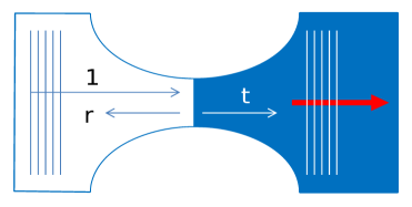
Figure 2: Schematic scattering problem of a phonon reflected and transmitted at the interface of a ferromagnet. The red arrow is the magnetization ($z$-) direction.

$$\chi_{L}^{\sigma}\left(z,t\right)=\frac{N_{p}^{L}}{k_{L}}\left[\left(\begin{array}[c]{c}0\\ 1\end{array}\right)e^{ik_{L}z}+\left(\begin{array}[c]{c}0\\ \mathfrak{r}_{L}^{\sigma}\end{array}\right)e^{-ik_{L}z}\right]e^{i\omega t},\;$$ (35)

where $N_{p}^{L}=\left(4\alpha_{L}^{3}\rho_{L}\right)^{-1/4},$ $k_{L}=v_{L}\omega=\sqrt{\alpha_{L}/\rho_{L}}\omega$ in terms of the acoustic parameters of the actuator and $\mathfrak{r}_{L}^{\sigma}$ is the reflection coefficient determined below. This state carries an energy flux of $F_{\sigma}=F_{0}^{\sigma}\left(1-\left|\mathfrak{r}_{L}^{\sigma}\right|^{2}\right),$ where $F_{0}^{\sigma}$ is the actuator power density. On the right side we can scatter into the two mixed eigenstates at the same frequency with transmission coefficients $\mathfrak{t}.$ The axial symmetry prevents mixing between states with different polarizations and

$$\chi_{R}^{\sigma}\left(z,t\right)=e^{i\omega t}\sum_{s}\mathfrak{t}_{s}^{\sigma}\left(\omega\right)\left(\begin{array}[c]{c}m_{s}^{\sigma}\\ r_{s}^{\sigma}\end{array}\right)e^{ik_{s}^{\sigma}z}$$ (36)

where the magnetic and lattice components are flux-normalized as described above. Energy conservation dictates that

$$\frac{F}{F_{0}}=1-\left|\mathfrak{r}_{L}^{\sigma}\right|^{2}=\sum_{s}\left|\mathfrak{t}_{s}^{\sigma}\right|^{2}$$ (37)

which reflects the unitarity of the scattering matrix composed by $\mathfrak{r}$ and $\mathfrak{t}$ (as well as by $\mathfrak{r}^{\prime}$ and $\mathfrak{t}^{\prime}$).

At the interface $z=0$ we demand continuity of the lattice $R^{\sigma}\left(0^{-}\right)=R^{\sigma}\left(0^{+}\right),$ which leads to

$$\frac{N_{p}^{L}}{k_{L}}\left(1+\mathfrak{r}_{L}^{\sigma}\right)=\sum_{s}\mathfrak{t}_{s}^{\sigma}r_{s}^{\sigma}.$$ (38)

Continuity of the stress or energy current at the interface $z=0$, $\bar{F}\left(0^{-}\right)=\bar{F}\left(0^{+}\right),$ leads to the boundary condition

$$\frac{b_{2}}{M_{0}}\sum_{s}\mathfrak{t}_{s}^{\sigma}m_{s}^{\sigma}=i\alpha_{L}\frac{N_{p}^{L}}{k_{L}}\left(1-\mathfrak{r}_{k_{L}}\right)-i\alpha_{R}\sum_{s}\mathfrak{t}_{s}^{\sigma}r_{s}^{\sigma}k_{s}^{\sigma}$$ (39)

Integrating the equation of motion over the interface leads to free boundary condition for the magnetization $\partial m^{\sigma}/\partial x\left(0^{+}\right)=0,$ which implies that the energy and angular momentum carried by spin waves vanish at the boundary, leading to a relation for the transmission coefficients

$$\sum_{s}\mathfrak{t}_{s}^{\sigma}m_{s}^{\sigma}k_{s}^{\sigma}=0$$ (40)

We have now three linear equations with three unknown variables for a choice of chirality, viz. $\mathfrak{t}_{1}^{\sigma},\,\mathfrak{t}_{2}^{\sigma}$ and $\mathfrak{r}_{L}^{\sigma}.\$We can easily derive the coefficients as analytic functions of $\omega$ and constituting parameters, but the expressions are lengthy, hence, not given here. We used parameters of gadolinium gallium garnet (GGG) for the actuator: $\rho_{L}=7085\,\mathrm{kg/m^{3}},\,\alpha_{L}=9.0\times 10^{10}\,\mathrm{Pa}$, which implies small but finite acoustic mismatch. In Fig. 3, the flux components at the interface are plotted as a function of frequency for the parameters used in the dispersion relations (Fig. 1).

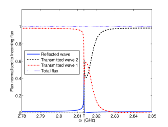
Figure 3: Normalized flux components $\left|\mathfrak{r}_{L}^{\sigma}\right|^{2},\left|\mathfrak{t}_{1}^{\sigma}\right|^{2},$ and $\left|\mathfrak{t}_{2}^{\sigma}\right|^{2}$ as a function of frequency close to the anticrossing between magnon and phonon modes. The labels of the transmitted waves are consistent with the labeling of the wave numbers in Fig. 1 (a) and (c). Flux conservation $\left|\mathfrak{r}_{L}^{\sigma}\right|^{2}+\left|\mathfrak{t}_{1}^{\sigma}\right|^{2}+\left|\mathfrak{t}_{2}^{\sigma}\right|^{2}=1$ is demonstrated. The FMR resonance frequency $\omega_{0}$ is indicated by the arrow on the abscissa.

Far from the (anti) crossing we observe weak reflection of the incoming sound wave, which is a consequence of the good acoustic impedance matching assumed here. Transmission into the phonon-like root $s$ that changes signs between low and high frequencies dominates. The transmission and reflection probabilities look complicated because the spin wave dispersion is so flat; the anticrossing overlaps with the FMR frequency $\omega_{0}$ for spin wave excitation, indicated by the arrow on the abscissa. This is so because the exchange energy at the anticrossing is insignificant as compared to the Zeeman energy. In the neighborhood of the anticrossing we observe the typical mode conversion plus an additional contribution to the back reflection of acoustic energy into the actuator.

5 Detection of magnetization dynamics by spin pumping

Uchida et al. [6] and Weiler et al. [7] detected the acoustically induced magnetization dynamics by the spin current pumped [8] into a thin layer of Pt with a significant spin Hall angle $\theta_{\mathrm{SH}}$ [22]. In terms of the spin mixing conductance $g_{r}^{\uparrow\downarrow}$ the magnitude and polarization of the spin current reads [8]

$$\mathbf{I}_{s}^{\mathrm{pump}} =\frac{\hbar}{4\pi}\frac{g_{r}^{\uparrow\downarrow}}{M_{0}^{2}}\mathbf{M}\times\frac{d\mathbf{M}}{dt}$$ (41)

$$=\frac{\hbar}{4\pi}\frac{g_{r}^{\uparrow\downarrow}}{M_{0}^{2}}\left(\begin{array}[c]{c}M_{0}\dot{M}_{x}\mathbf{\hat{y}}-M_{0}\dot{M}_{y}\mathbf{\hat{x}}\\ +\left(M_{x}\dot{M}_{y}-M_{y}\dot{M}_{x}\right)\mathbf{\hat{z}}\end{array}\right).$$ (44)

For $M_{x}^{2}+M_{y}^{2}\ll M_{0}^{2}$ the average cone angle

$$\Theta =\sqrt{\left\langle M_{x}^{2}+M_{y}^{2}\right\rangle_{z,t}}/M_{0}$$ (45)

$$=2\sqrt{\sum_{s}\left(\left|t_{s}^{+}\right|^{2}\left|m_{s}^{+}\right|^{2}+\left|t_{s}^{-}\right|^{2}\left|m_{s}^{-}\right|^{2}\right)}/M_{0}$$ (46)

is a convenient metric for the excitation of the magnetic degree of freedom per unit acoustic energy flux. The angular brackets indicate a time and position average over interference fringes that are an artifact of the one-dimensional and monochromatic approximations. $\Theta\left(\omega\right)$ is plotted in Fig. 4. The qualitative features can be understood in terms of competition between magnetic character and excitation efficiency of the eigenmodes. As the frequency approaches the anticrossing from below, the increasing magnetic character of the propagating normal mode leads to an increasing $\Theta$. Just below the FMR frequency, the normal mode becomes flat, corresponding to a small group velocity which reduces mode excitation efficiency (see Fig. 3). Just above the FMR frequency, a new propagating normal mode becomes available which restores a relatively efficient mode excitation. The highest $\Theta$ is achieved close to the crossing at which the acoustic and magnetic modes are fully mixed. Finite dissipation, finite quality factor of the actuator, and disorder disregarded here will broaden the sharp features and reduce the magnetization amplitude, but the effects are believed to be minor for high quality YIG and proper actuator design.

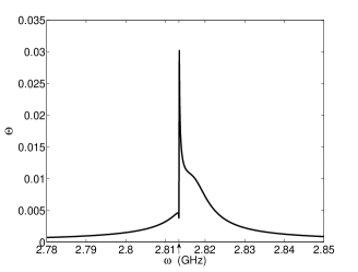
Figure 4: $\Theta$ (Eq. (45)) vs. frequency of the injected sound wave for unit injected acoustic energy $F_{0}=1\,\mathrm{J/}\left(\mathrm{m}^{2}\mathrm{s}\right)$ ($\Theta\sim\sqrt{F_{0}}$) . $\Theta$ is the average precession cone angle and a metric for the efficiency of acoustic excitation of the magnetic degree of freedom. The FMR resonance frequency $\omega_{0}$ is indicated by the arrow on the abscissa.

When the Hall contacts of the Pt layer are short circuited, the spin current induces a Hall charge current in the Pt layer with direction and magnitude [22]

$$\mathbf{I}_{c}=\frac{2e}{\hbar}\theta_{\mathrm{SH}}\mathbf{\hat{z}}\times\mathbf{I}_{s}^{\mathrm{pump}}$$ (47)

with

$$\left(\mathbf{I}_{c}\right)_{x,y} =-\frac{eg_{r}^{\uparrow\downarrow}}{2\pi}\theta_{SH}\frac{\dot{M}_{x,y}}{M_{0}}$$ (48)

$$\sqrt{\left\langle\left|\left(\mathbf{I}_{c}\right)_{x}\right|^{2}+\left|\left(\mathbf{I}_{c}\right)_{y}\right|^{2}\right\rangle} =\frac{eg_{r}^{\uparrow\downarrow}\theta_{SH}}{2\pi M_{0}}\sqrt{\left\langle(\dot{M}_{x})^{2}\right\rangle+\left\langle(\dot{M}_{y})^{2}\right\rangle}$$ (49)

$$=\frac{eg_{r}^{\uparrow\downarrow}\theta_{SH}\omega\Theta}{2\pi}.$$ (50)

We see that the DC spin current component does not generate an inverse spin Hall effect in this configuration, but a pure AC inverse spin Hall effect is expected [17]. The currents in the $x$ and $y$-direction oscillate at the frequency of the actuating ultrasound with amplitude $\sim\Theta,$ in contrast to the DC inverse spin Hall effect that scales with $\Theta^{2}$ and is orders of magnitude smaller for small acoustic energy fluxes. The FMR generated AC inverse spin Hall effect is difficult to observe since the Pt layer is directly subjected to rf radiation, which causes strong electrodynamic artifacts at the resonance frequency. The acoustically generated AC inverse spin Hall effect does not suffer from this disadvantage when the piezoelectric material is spatially separated from the magnetic material.

6 Conclusions

We computed the acoustically stimulated magnetization dynamics and the associated spin-pumping induced ac inverse spin Hall effect for a symmetric configuration of transverse acoustic waves polarized normal to the magnetization direction. The theory can be extended to include longitudinal phonons (pressure waves) and arbitrary magnetization direction, finite quality factor of the actuator, finite magnetizations damping, multilayered structures, diffuse scattering by disorder, etc., if necessary. In principle this formalism can be extended as well to obtain spin and heat transport through arbitrary structures under a temperature difference between the reservoirs by including incoming and outgoing waves with all wave vectors.

References

• [1] C. Kittel, Introduction to Solid State Physics, (John Wiley, Hoboken, 2005).
• [2] A. Einstein and W. J. de Haas, Deutsche Physikalische Gesellschaft, Verhandlungen 17, 152 (1915).
• [3] S. J. Barnett, Phys. Rev. 6, 239 (1915); S. J. Barnett, Rev. Mod. Phys. 7, 129 (1935).
• [4] C. Kittel, Phys. Rev. 110, 836 (1958).
• [5] S. Chikazumi, Physics of Ferromagnetism, (Oxford University Press, Oxford, 1997).
• [6] K. Uchida, H. Adachi, T. An, T. Ota, M. Toda, B. Hillebrands, S. Maekawa, and E. Saitoh, Nat. Mater. 10, 737 (2011).
• [7] M. Weiler, H. Huebl, F. S. Goerg, F. D. Czeschka, R. Gross, and S. T. B. Goennenwein, Phys. Rev. Lett. 108, 176601 (2012).
• [8] Y. Tserkovnyak, A. Brataas, and G. E.W. Bauer, Phys. Rev. Lett. 88, 117601 (2002).
• [9] E. Saitoh, M. Ueda, H. Miyajima, and G. Tatara, Appl. Phys. Lett. 88, 182509 (2006).
• [10] T. Kobayashi, R. C. Barker, J. L. Bleustein, and A. Yelon, Phys. Rev. B 7, 3273 (1973).
• [11] L. Dreher, M. Weiler, M. Pernpeintner, H. Huebl, R. Gross, M. S. Brandt, and S. T. B. Goennenwein, Phys. Rev. B 86, 134415 (2012).
• [12] H. Boemmel and K. Dransfeld, Phys. Rev. Lett. 3, 83 (1959).
• [13] I. Feng, M. Tachiki, C. Krischer, and M. Levy, J. Appl. Phys. 53, 177 (1982).
• [14] H. F. Tiersten, J. Math. Phys. 5, 1298 (1964).
• [15] S. Datta, Electronic Transport in Mesoscopic Systems, (Cambridge University Press, Cambridge, 2003).
• [16] Y.V. Nazarov and Y.M. Blanter, Quantum Transport: Introduction to Nanoscience, (Cambridge University Press, Cambridge, 2009).
• [17] H. Jiao and G.E.W. Bauer, Phys. Rev. Lett. 110, 217602 (2013).
• [18] F. G. Eggers and W. Strauss, J. Appl. Phys. 34, 1180 (1963).
• [19] P. Hansen, Phys. Rev. B 8, 246 (1973).
• [20] YIG Crystal Specification Sheet, Deltronic Crystal Industries (Inc.), http://deltroniccrystalindustries.com .
• [21] A. Akhiezer, V. Bar’yakhtar, and S. Peletminskii, Spin Waves (North Holland Publishing Company, Amsterdam 1968).
• [22] A. Hoffmann, IEEE Trans. Magn. 49, 5172 (2013).