Turbulent velocity spectra in a quantum fluid:
experiments, numerics and models

Abstract

Turbulence in superfluid helium is unusual and presents a challenge to fluid dynamicists because it consists of two coupled, inter penetrating turbulent fluids: the first is inviscid with quantised vorticity, the second is viscous with continuous vorticity. Despite this double nature, the observed spectra of the superfluid turbulent velocity at sufficiently large length scales are similar to those o ordinary turbulence. We present experimental, numerical and theoretical results which explain these similarities, and illustrate the limits of our present understanding of superfluid turbulence at smaller scales.

I Motivations

If cooled below a critical temperature ($T_{\lambda}\approx 2.18\,$K in ⁴He and $T_{\rm c}\approx 10^{-3}\,K$ in at ³He at saturated vapour pressure), liquid helium undergoes Bose-Einstein condensation Annett , becoming a quantum fluid and demonstrating superfluidity (pure inviscid flow). Besides the lack of viscosity, another major difference between superfluid helium and ordinary (classical) fluids such as water or air is that, in helium, vorticity is constrained to vortex line singularities of fixed circulation $\kappa=h/M$, where $h$ is Planck’s constant, and $M$ is the mass of the relevant boson (in the most common isotope ⁴He, $M=m_{4}$, the mass of an atom; in the rare isotope ³He, $M=2\,m_{3}$, the mass of a Cooper pair). These vortex lines are essentially one-dimensional space curves, like the vortex lines of fluid dynamics textbooks; for example, in ⁴He the vortex core radius $\xi\approx 10^{-10}$m is comparable to the inter atomic distance. This quantisation of the circulation thus results in the appearance of another characteristic length scale: the mean separation between vortex lines, $\ell$. In typical experiments (both in ⁴He and ³He) $\ell$ is orders of magnitude smaller than the outer scale of turbulence $D$ (the scale of the largest eddies) but is also orders of magnitudes larger than $\xi$.

There is a growing consensus Skrbek-Sreeni-2012 that on length scales much larger than $\ell$ the properties of superfluid turbulence are similar to those of classical turbulence if excited similarly, for example by a moving grid. The idea is that motions at scales $R\gg\ell$ should involve at least a partial polarization Hulton ; Laurie-2012 of vortex lines and their organisation into vortex bundles which, at such large scales, should mimic continuous hydrodynamic eddies. Therefore one expects a classical Richardson-Kolmogorov energy cascade, with larger “eddies” breaking into smaller ones. The spectral signature of this classical cascade is indeed observed experimentally in superfluid helium. In the absence of viscosity, in superfluid turbulence the kinetic energy should cascade downscale without loss, until it reaches the small scales where the quantum discreteness of vorticity is important. It is also believed that at this point the Richardson-Kolmogorov eddy-dominated cascade should be replaced by a second cascade which arises from the nonlinear interaction of Kelvin waves (helical perturbation of the vortex lines) on individual vortex lines. This Kelvin wave cascade should take the energy further downscale where it is radiated away by thermal quasi particles (phonons and rotons in ⁴He).

Although this scenario seems quite reasonable, crucial details are yet to be established. Our understanding of superfluid turbulence at scales of the order of $\ell$ is still at infancy stage, and what happens at scales below $\ell$ is a question of intensive debates. The “quasi-classical” region of scales, $R\gg\ell$, is better understood, but still less than classical hydrodynamic turbulence. The main reason is that at nonzero temperatures (but still below the critical temperature $T_{\lambda}$), superfluid helium is a two-fluid system. According to the theory of Landau and Tisza Donnelly , it consists of two inter–penetrating components: the inviscid superfluid, of density $\rho_{\text{s}}$ and velocity ${\bf{u}}_{\text{s}}$ (associated to the quantum ground state), and the viscous normal fluid, of density $\rho_{n}$ and velocity $\bm{u}_{\text{n}}$ (associated to thermal excitations). The normal fluid carries the entropy $S$ and the viscosity $\mu$ of the entire liquid. In the presence of superfluid vortices these two components interact via a mutual friction forceBDV1982 . The total helium density $\rho=\rho_{\text{s}}+\rho_{n}\approx~{}145~{}\rm kg/m^{3}$ is practically temperature independent, while the superfluid fraction $\rho_{\text{s}}/\rho$ is zero at $T=T_{\lambda}$, but rapidly increases if $T$ is lowered (it becomes 50% at $T\approx 2~{}\rm K$, 83% at $T\approx 1.6~{}\rm K$ and 95% at $T\approx 1.3~{}\rm K$ DB ). The normal fluid is essentially negligible below $1~{}\rm K$. One would therefore expect classical behaviour only in the high temperature limit $T\to T_{\lambda}$, where the normal fluid must energetically dominate the dynamics. Experiments show that this is not the case, thus raising the interesting problem of “double-fluid” turbulence which we study here.

The aim of this article is to present the current state of the art in this intriguing problem, clarify common features of turbulence in classical and quantum fluids, and highlight their differences. To achieve our aim we shall overview and combine experimental, theoretical and numerical results in the simplest possible (and, probably, the most fundamental) case of homogeneous, isotropic turbulence, away from boundaries and maintained in a statistical steady state by continuous mechanical forcing. The natural tools to study homogeneous isotropic turbulence are spectral, thus we shall consider the velocity spectrum (also known as the energy spectrum) and attempt to give a physical explanation for the observed phenomena.

II Classical vs. superfluid turbulence

We recall that ordinary incompressible viscous flows are described by the Navier-Stokes equation

$$\Big{[}\frac{\partial\,\bf u}{\partial t}+({\bf{u}}\cdot{\bf{\nabla}}){\bf{u}}\Big{]}=-\frac{1}{\rho}{{\bf{\nabla}}p}+\nu{{\bf{\nabla}}^{2}}{\bf{u}},$$ (1)

and the solenoidal condition ${\bf{\nabla}}\cdot{\bf{u}}=0$ for the velocity field ${\bf{u}}$, where $p$ is the pressure, $\rho$ the density, and $\nu=\mu/\rho$ the kinematic viscosity. The dimensionless parameter that determines the properties of hydrodynamic turbulence is the Reynolds number Re$=VD/\nu$. The Reynolds number estimates the ratio of nonlinear and viscous terms in Eq. (1) at the outer length scale $D$ (typically the size of a streamlined body), where $V$ is the root mean square turbulent velocity fluctuation. In fully developed turbulence (Re$\gg 1$) the $D$-scale eddies are unstable and give birth to smaller scale eddies, which, being unstable, generate further smaller eddies, and so on. This process is the Richardson-Kolmogorov energy cascade toward eddies of scale $\eta$, defined as the length scale at which the nonlinear and viscous forces in Eq. (1) approximately balance each other. $\eta$-scale eddies are stable and their energy is dissipated into heat by viscous forces. The hallmark feature of fully developed turbulence is the coexistence of eddies of all scales from $D$ to $\eta\simeq D{\rm Re}^{-3/4}\ll D$ with universal statistics; the range of length scales $D\ll R\ll\eta$ where both energy pumping and dissipation can be ignored is called the inertial range.

In the study of homogeneous turbulence it is customary to consider the energy density per unit mass $E(t)$ (of dimensions $\rm m^{2}/s^{2}$). In the isotropic case the energy distribution between eddies of scale $R$ can be characterized by the one–dimensional energy spectrum $E(k,t)$ of dimensions $\rm m^{2}/s^{2}$) with wavenumber defined as $k=2\pi/R$ (or as $k=1/R$), normalized such that

$$E(t)=\frac{1}{\cal V}\int\frac{1}{2}{{\bf{u}}}^{2}d{\cal V}=\int_{0}^{\infty}E(k,t)dk,$$

where ${\cal V}$ is volume. In the inviscid limit, $E(t)$ is a conserved quantity ($dE(t)/dt=0$), thus $E(k,t)$ satisfies the continuity equation

$$\frac{\partial E(k,t)}{\partial t}+\frac{\partial\varepsilon(k,t)}{\partial k}=0,$$ (2)

where $\varepsilon(k,t)$ is the energy flux in spectral space (of dimensions $\rm m^{2}/s^{3}$). In the stationary case, energy spectrum and energy flux are $t$–independent, thus Eq. (2) immediately dictates that the energy flux $\varepsilon$ is $k$-independent. Assuming that this constant $\varepsilon$ is the only relevant characteristics of turbulence in the inertial interval and using dimensional reasoning, in 1941 Kolmogorov and (later) Obukhov suggested that the energy spectrum is

$$E_{\text{K41}}(\varepsilon,k)=C_{\scriptscriptstyle\rm{K41}}\varepsilon^{2/3}k^{-5/3},$$ (3)

where the (dimensionless) Kolmogorov constant is approximately $C_{\scriptscriptstyle\rm{K41}}\approx 1$. This is the celebrated Kolmogorov-Obukhov $5/3$ law (KO–41), verified in experiments and numerical simulations of Eq. (1); it states in particular that in incompressible, steady, homogeneous, isotropic turbulence, the distribution of kinetic energy over the wavenumbers is $E(k)\propto k^{-5/3}$.

In the inviscid limit the energy flux goes to smaller and smaller scales, reaching finally the interatomic scale and accumulating there. To describe this effect, Leith Leith67 suggested to replace the algebraic relation (3) between $\varepsilon(k)$ and $E(k)$ by the differential form:

$$\varepsilon(k)=-{1\over 8}\,\sqrt{k^{11}E(k)}\ {d\,\over dk}\left(\frac{E(k)}{k^{2}}\right)\ .$$ (4)

This approximation dimensionally coincides with Eq. (3), but the derivative $d[E(k)/k^{2}]/dk$ guarantees that $\varepsilon(k)=0$ if $E(k)\propto k^{2}$. The numerical factor $1/8$, suggested in Nazar-Leith , fits the experimentally observed value $C_{\scriptscriptstyle\rm{K41}}=(24/11)^{2/3}\approx 1.7$ in Eq. (3).

A generic energy spectrum with a constant energy flux was found in Nazar-Leith as a solution to the equation  $\varepsilon(k)=\varepsilon$ constant:

$$E(\varepsilon,k)=C_{\scriptscriptstyle\rm{K41}}\frac{\varepsilon^{2/3}}{k^{5/3}}T_{\text{eq}}(k)\,,$$ (5)

$$T_{\text{eq}}(k)=\left[1+\Big{(}\frac{k}{k_{\text{eq}}}\Big{)}^{11/2}\right]^{2/3}.$$

Notice that at low $k$, Eq. (5) coincides with KO–41, while for $k\gg k_{\text{eq}}$ it describes a thermalized part of the spectrum, $E(k)\propto k^{2}$, with equipartition of energy (shown by the solid black line at the right of in Fig. 3A, and, underneath in the same figure, by the solid red line, although the latter occurs in slightly different contexts) .

We shall have also to keep in mind that although Eq. (3) is an important result of classical turbulence theory, it presents only the very beginning of the story. In particular, its well known Frisch that in the inertial range, the turbulent velocity field is not self–similar, but shows intermittency effects which modify the KO–41 scenario.

In this paper we apply these ideas to superfluid helium, explain how to overcome technical difficulties to measure the energy spectrum near absolute zero, and draw the attention to three conceptual differences between classical hydrodynamic turbulence and turbulence in superfluid ⁴He.

The first difference is that the quantity which (historically) is most easily and most frequently detected in turbulent liquid helium is not the superfluid velocity but rather the vortex line density $\cal L$, defined as the superfluid vortex length per unit volume; in most experiments (and numerical simulations) this volume is the entire cell (or computational box) which contains the helium. This scalar quantity $\cal L$ has no analogy in classical fluid mechanics and should not be confused with the vorticity, whose spectrum, in the classical KO–41 scenario, scales as $k^{1/3}$ correspondingly to the $k^{-5/3}$ scaling of the velocity. Notice that in a superfluid the vorticity is zero everywhere except on quantized vortex lines. In order to use as much as possible the toolkit of ideas and methods of classical hydrodynamics, we shall define in the next sections an ”effective” superfluid vorticity field ${\mbox{\boldmath$\omega$}}_{s}$; this definition (which indeed Baggaley-structures yields the classical $k^{1/3}$ vorticity scaling corresponding to the $k^{-5/3}$ velocity scaling) is possible on scales that exceed the mean intervortex scale $\ell$, provided that the vortex lines contained in a fluid parcel are sufficiently polarized. This procedure opens the way for a possible identification of ”local” values of ${\cal L}({\bf{r}},t)$ with the magnitude $|{\mbox{\boldmath$\omega$}}_{s}|$ of the vector field ${\mbox{\boldmath$\omega$}}_{s}$.

The second difference is that liquid helium is a two fluid system, and we expect both superfluid and normal fluid to be turbulent. This makes the problem of superfluid turbulence much richer than classical turbulence, but the analysis becomes more involved. For example, the existence of the intermediate scale $\ell$ makes it impossible to apply arguments of scale invariance to the entire inertial interval and calls for its separation into three ranges. The first is a “hydrodynamic” region of scales $\ell\ll R\ll D$ (corresponding to $k_{D}\ll k\ll k_{\ell}$ in k-space where $k_{D}=2\pi/D$ and $k_{\ell}=2\pi/\ell$), which is similar (but not equal) to the classical inertial range; the second is a “Kelvin wave region” $\xi\ll R\ll\ell$ where energy is transferred further to smaller scales by interacting Kelvin waves (helix-like deformations of the vortex lines). In the third, intermediate region $R\approx\ell$, the energy flux is caused probably by vortex reconnections.

Finally, the third difference is that mutual friction between normal and superfluid components leads to (dissipative) energy exchange between them in either direction.

Studies of classical turbulence are solidly based on the Navier-Stokes Eq. (1). Unfortunately, there are no well established equations of motion for ⁴He in the presence of superfluid vortices. We have only models at different levels of description (for an overview see Sec. IV). All these issues make the problem of superfluid turbulence very interesting from a fundamental view point, simultaneously creating serious problems in experimental, numerical and analytical studies.

A	B

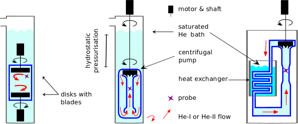
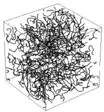
Figure 1: Panel A: Examples of flows sustaining steady turbulence in superfluid ⁴He for which spectral measurements were performed. From left to right : Von Karman flows (Tabeling ; Schmoranzer-2009 ; SHREK ), wind-tunnels (Salort-EPL-2012 ; Roche-2007 ) and pressurised circulator cooled through a heat exchanger Salort-2010 . Panel B: Snapshot of a vortex tangle calculated using the Vortex Filament Method (VFM) in a periodic box Sherwin-2013 .

III Experiments: flows, probes and spectra

In this section we shall limit our discussion to experimental techniques for ⁴He. The methods used in ³He, at temperatures which are one thousand times smaller, are rather different Fisher-Udine , and we shall only cite the results in ³He which are directly relevant to our aim.

Possibly the simplest method to generate turbulence in ⁴He is the application of a temperature gradient which creates a flow of the normal component carrying heat from the hot to the cold plate; this flow is compensated by the counterflow of the superfluid component in the opposite direction which maintains a zero mass flux. This form of heat conduction, called thermal counterflow, is unlike what happens in ordinary fluids. Moreover, under thermal drive, the energy pumping is dominated by the intervortex length scale $\ell$ and according to numerical simulations there is no inertial interval in which the energy flux scales over the wavenumbers as in the KO–41 scenario Sherwin-2012 . The resulting “quantum” superfluid turbulence Nemirovskii:PhysRep2013 is thus very different from classical turbulence at large level of drive and will not be discussed here.

From the experimental point of view, the generation of turbulence by mechanical means (more similar to what is done in the study of ordinary turbulence) is not as straightforward. Nevertheless, the literature reports a number of successful approaches, which can be classified into three main categories: (i) flows driven by vibrating objects, (ii) one-shot-flows driven by single-stroke-bellows, towed grids or spin-up/down of the container, and (iii) flows continuously driven by propellers. Most efforts in characterising the turbulent fluctuations have focused on the third category. The reason is simple: the resulting turbulent flows do not suffer from the lack of homogeneity and isotropy which is typical of the flows generated by vibrating objects, and allow better statistical convergence (and improved stationarity) than measurements in non-stationary flows.

To illustrate the different cryogenics experimental set-ups, it is useful to distinguish between the two liquid phases of ⁴He: liquid helium I (He-I) and helium II (He-II), respectively above $T_{\lambda}$ and below $T_{\lambda}$. The former is an ordinary viscous fluid, the latter is the quantum fluid of interest here. Since He-II is created by cooling He-I, in most cases the same apparatus or experimental technique can be used to probe classical as well as quantum turbulence, which helps making comparisons.

Panel A in Fig. 1 illustrates three different flow arrangements which have enabled spectral measurements of velocity and vortex line density. The configuration on the left is inspired by the historical experiment of Tabeling and collaborators Tabeling in which helium was driven by two counter-rotating propellers attached to motors operating at cryogenic temperature (or at room temperature in more recent experiments Schmoranzer-2009 ; SHREK ). The configuration in the middle is the TOUPIE wind-tunnel Salort-EPL-2012 which upgrades a smaller wind-tunnel Roche-2007 . A 1-m-high column of liquid ⁴He pressurises hydrostatically the bottom wind-tunnel section to allow operation in He-I up to velocities of 4 m/s without the occurrence of cavitation (prevented by the high thermal conductivity of superfluid helium below the superfluid transition). Without a dedicated pressurisation system, the bubbles which would form in He I above $T_{\lambda}$ would prevent the comparison of turbulence above and below the superfluid transition in the same apparatus. The configuration at the right illustrates the TSF circulator, which consists of a pressurised helium loop cooled by a heat exchanger Salort-2010 . All these flows are driven by the centrifugal force generated by propellers: such forcing does not rely on viscous nor thermal effects and is therefore well fitted to liquid helium irrespectively of its superfluid density fraction.

A	B	C

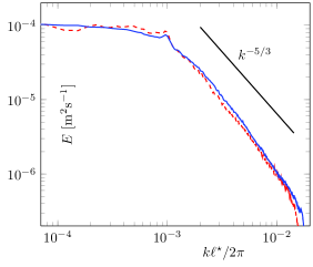
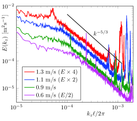
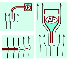
Figure 2: Color online. Measured spectra of superfluid turbulence in ⁴He. All cut-off at high $k$ or $f$ are caused by the resolution of the probes. Panel A: Energy spectrum measured in the TOUPIE wind-tunnel below the superfluid transition (solid blue line, 1.56 K$<T_{\lambda}$) and above $T_{\lambda}$ (dashed red line) Salort-EPL-2012 . Above $T_{\lambda}$, the parameter $\ell^{\star}$ on the x-axis is chosen such that the small peak separating the inertial scales plateau and the cascade matches the one estimated below $T_{\lambda}$ at $k_{z}\ell/2\pi=10^{-3}$ (this peak is associated with eddy shedding from the cylinder used upstream to generate turbulence). Panel B: Energy spectra for different mean flow velocities for $T=1.55~{}{\rm K}$ in a smaller He-II wind tunnel. An arbitrary vertical offset had been introduced for clarity (see legend). Panel C: Local velocity probes used in superfluid ⁴He for measurements of fluctuations at sub-millimetre scales. Stagnation pressure velocity probes without static pressure reference (top-left) (Tabeling ; Salort-2010 ), stagnation pressure velocity probe with a static pressure reference (right) (Salort-2010 ; Salort-EPL-2012 ), and cantilever-based velocity probe (bottom left) Salort-RSI-2012 .

Experience shows that probing cryogenic flows is often more challenging than producing the flow themselves, partly because dedicated probes often have to be designed and manufactured for each experiment. This is all the more true if good space and time resolutions are required to resolved the fluctuating scales of superfluid turbulence.

Below $T_{\lambda}$, the most commonly-used local velocity probe is based on the principle of the “Pitot” or “Prandtl” tube (sometimes called “total head pressure” tube), which is illustrated in the top-left and right sketches of Fig. 2C. One end of a tube is inserted parallel to the mean flow, while the other end is blocked by a pressure gauge. The stagnation point which forms at the open end of the tube is associated with an overpressure probed by the gauge. This stagnation-point overpressure $P$ is related to the incoming flow velocity $V$ using Bernoulli relation $P\simeq\rho V^{2}/2$. In the arrangement depicted in the right sketch of Fig. 2C, the use of a differential pressure probe allows to remove the “static” pressure variation of the flow associated with turbulent pressure fluctuations and acoustical background noise. The operation of such stagnation-pressure probes below the critical temperature and their limitations are discussed in Ref. Salort-2010 . In summary, the fluctuations $\delta P$ of $P$ are proportional to the fluctuations $\delta V$ of $V$ up to the second order term in $(\delta V/V)^{2}$ and the mean flow direction has to be well defined (excessive angles of attack lead to measurement bias). Pitot tubes achieving nearly 0.5-mm spatial resolution, and others with DC-4 kHz bandwidth have been operated successfully. At such scales and in the turbulent flows of interest, helium’s two components are expected to be locked together -as discussed later- and described by a single continuous fluid of total density $\rho$. Therefore stagnation pressure probes determine the common velocity of both fluid components.

The first experimental turbulent energy spectra below $T_{\lambda}$ were reported in 1998 Tabeling using the set-up illustrated in Fig. 1A-left. Energy spectra at 2.08 K and 1.4 K were found very similar to the spectrum measured in He I above the superfluid transition, at 2.3 K. In the range of frequencies corresponding to the length scale of the forcing scale and the smallest resolved length scale, the measured spectrum was compatible with KO–41. The next published confirmation of Kolmogorov’s law came in 2010 Salort-2010 from two independent wind-tunnels of the types depicted in the centre and at the right-side of Fig. 1A. Measurements obtained with the first type of wind-tunnel are reproduced in Fig. 2B, which shows energy spectra at 1.6 K for various mean velocities of the flow. We note that four decades separate the integral scale of the flow ($D\simeq$ 10 mm) and the intervortex scale $\ell\simeq 1\rm\mu m$, to be compared with the 1 mm effective resolution of the anemometer. Measurements obtained with the second type of wind-tunnel explored grid turbulence. Although the signal-to-noise ratio was not as good, the choice of a well-defined flow allowed to estimate independently both prefactors of Eq. (3): the Kolmogorov constant $C_{\scriptscriptstyle\rm{K41}}$ and the dissipation rate $\varepsilon$. Within accuracy (30% for $C_{\scriptscriptstyle\rm{K41}}$), it was found that both prefactors were similar above the superfluid transition and below it in He-II at $T=2.0~{}\rm K$. The energy spectrum shown in Fig. 2A has been recently obtained in the TOUPIE experiment both above and below $T_{\lambda}$ in the far wake of a disc. To normalise the x-axis of this plot, the mean intervortex distance $\ell$ in He-II was estimated using the relation $2{\ell}/{D}=$Re${}_{\kappa}^{-3/4}$ Salort-2011 where ${\rm Re}_{\kappa}=DV/\kappa$ is a Reynolds number defined using the root mean square velocity from the anemometer, and the prefactor $2$ was fitted to experimental and numerical data in the range $T\simeq 1.4-1.6\,K$.

The high signal-to-noise ratio of this dataset allowed to check the validity of the $-4/5$ Karman-Howarth law Salort-EPL-2012 . This law, sometimes described as the only exact relation known in turbulence, confirms that energy cascades from large to small scales without dissipation within the inertial range where the KO–41 scaling is observed.

Finally, it should be noticed that intermittency of velocity fluctuations were partially explored in two experimental studies Tabeling ; SalortIntermi:ETC13_2011 , but no specific signature of superfluid turbulence was reported. Both studies only explored the high and low temperature regimes ($\rho_{\text{s}}/\rho_{\text{n}}\simeq 0.29$ at $T=2.08\,K$ and $\rho_{\text{s}}/\rho>0.85$ at $T\leq 1.56\,K$).

In all published energy spectra, the limited resolution of the anemometer is responsible for the cut-off at high frequency/small scale. Thus, the observed spectra reveal only “half” of the picture, namely the integral scales and the upper half of the inertial scales. To circumvent this limitation in resolution, a first approach is to scale up the experiment (at given Reynolds number $Re_{\kappa}$) so that all characteristic flow scales are magnified and better resolved with existing probes. This approach has been undertaken with the construction of a 78-cm diameter He-II Von Karman flow in Grenoble SHREK that is one order of magnitude larger than the 1998’s reference cell. Another approach is to scale down the probes. For practical reasons it is difficult to miniaturise much further stagnation pressure probes without a significant decrease of their sensibility or time response. New types of anemometers need to be invented. One possibility arises from the recent development of fully micro-machined anemometers based on the deflection of a silicon cantilever (see the bottom left sketch of Fig. 2C). Preliminary spectral measurements with a resolution of $100\rm\mu m$ have been recently reported in a He-II test facility Salort-RSI-2012 .

A	B	C

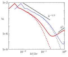
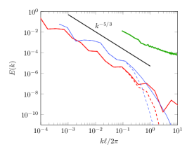
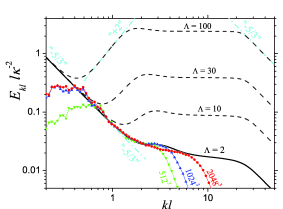
Figure 3: Color online. Numerical superfluid energy spectra vs normalised wavenumber for three hierarchical levels of motion Eqs. (9), (8) and (7): Panel A: Superfluid (solid line) and normal fluid (dashed line) energy spectra from simulation of the HVBK equations (9) at $T=1.15~{}\rm K$ (red) and $\simeq$2.16 K (blue) with truncation of phase space beyond the intervortex scale Salort-EPL-2012 . Panel B: Superfluid energy spectrum from VFM simulations  (8) at $T=2.164~{}\rm K$ (solid green line) Sherwin-2013 with synthetic turbulence prescribed for the normal component. Superfluid (red/blue solid line) and normal fluid (red/blue dashed line) energy spectra from shell model simulation of the HVBK equations at 1.44 K (red) and 2.157 K (blue) Wacks-2011 . Panel C: Superfluid energy spectrum from GPE simulations (7) complemented by dissipation at high $k$ Sasa-2011 . The numerical resolution is 2048³ (red line), 1024³ (dashed blue line) and 512³ (green dots). The intervortex distance $\ell$ results from a fit of the data (see original publication). In all panels, the normalisation of the x-axis (wavevector $k$) highlights the mean intervortex distance $\ell$. Black dashed lines show analytical predictions of the bottleneck LNR-2 discussed in Sec. 8A with different $\Lambda=\ln(\ell/\xi)$. The black solid line with $\Lambda=2$ corresponds to the simulation in Ref. Sasa-2011 . The dashed cyan lines show (from the left) the KO–41 (-5/3) scaling, the energy equipartition scaling ($+2$) and, at the right, the (-5/3) LN spectrum Eq. (13).

IV Equations of motion: three levels of description.

In the absence of superfluid vortices, Landau’s two-fluid equationsDonnelly for the superfluid and normal fluid velocities ${\bf{u}}_{\text{s}}$ and ${\bf{u}}_{\text{n}}$ account for all phenomena observed in He-II at low velocities, for example second sound and thermal counterflow. In the incompressible limit (${{\bf{\nabla}}}\cdot{{\bf{u}}_{\text{s}}}=0$, ${{\bf{\nabla}}}\cdot{{\bf{u}}_{\text{n}}}=0$) Landau’s equations are:

$$\Big{[}(\partial\,{\bf{u}}_{\text{s}}/\partial t)+({\bf{u}}_{\text{s}}\cdot{\bf{\nabla}}){\bf{u}}_{\text{s}}\Big{]} = -{\bf{\nabla}}p_{s}/\rho_{s},$$ (6a)

$$\Big{[}(\partial\,{\bf{u}}_{\text{n}}/\partial t)+({\bf{u}}_{\text{n}}\cdot{\bf{\nabla}}){\bf{u}}_{\text{n}}\Big{]} = -{\bf{\nabla}}p_{n}/\rho_{n}+\nu_{n}\nabla^{2}{{\bf{u}}_{\text{n}}}\,,$$ (6b)

where $\nu_{n}=\mu/\rho_{n}$ is the kinematic viscosity, and the efficient pressures $p_{s}$ and $p_{n}$ are defined by ${{\bf{\nabla}}}p_{s}=(\rho_{s}/\rho){{\bf{\nabla}}}p-\rho_{s}S{{\bf{\nabla}}}T$ and ${{\bf{\nabla}}}p_{n}=(\rho_{n}/\rho){{\bf{\nabla}}}p+\rho_{s}S{{\bf{\nabla}}}T$. On physical ground, Laudau argued that the superfluid is irrotational.

The main difficulty in developing a theory of superfluid turbulence is the lack of an established set of equations of motion for He-II in the presence of superfluid vortices. We have only models at different levels of description.

IV.1 First level

At the first, most microscopic level of description, we must account for phenomena at the length scale of the superfluid vortex core, $R\approx\xi$. Monte Carlo models of the vortex core Reatto , although realistic, are not suitable for the study of the dynamics and turbulent motion. A practical model of a pure superfluid is the Gross-Pitaevskii Equation (GPE) for a weakly-interacting Bose gas Annett :

$$i\hbar\frac{\partial\Psi}{\partial t}=-\frac{\hbar^{2}}{2M}\nabla^{2}\Psi+V_{0}|\Psi|^{2}\Psi-E_{0}\Psi\,,$$ (7)

where $\Psi({\bf{r}},t)$ is the complex condensate’s wave function, $V_{0}$ the strength of the interaction between bosons, $E_{0}$ the chemical potential and $M$ the boson mass. The condensate’s density $\tilde{\rho_{s}}$ and velocity $\tilde{{\bf{v}}_{\text{s}}}$ are related to $\Psi=|\Psi|\exp(i\Theta)$ via the Madelung transformation $\tilde{\rho_{s}}=M|\Psi|^{2}\,,\quad\tilde{{\bf{u}}_{\text{s}}}=\hbar{\bf{\nabla}}\Theta/M$, which confirms Landau’s intuition that the superfluid is irrotational. It can be shown that, at length scales $R\gg\xi=\hbar/\sqrt{2ME_{0}}$, the GPE reduces to the classical continuity equation and the (compressible) Euler equation. It must be stressed that, although the GPE accounts for quantum vortices, finite vortex core size (of the order of $\xi$), vortex nucleation, vortex reconnections, sound emission by accelerating vortices and Kelvin waves, it is only a qualitative model of the superfluid component. He-II is a liquid, not a weakly-interacting gas, and the condensate is only a fraction of the superfluid density $\rho_{s}$. No adjustment of $V_{0}$ and $E_{0}$ can fit both the sound speed and the vortex core radius, and the dispersion relation of the uniform solution of Eq. (7) lacks the roton’s minimum which is characteristic of He-II Donnelly . This is why, strictly speaking, we cannot identify $\tilde{\rho_{s}}$ with $\rho_{s}$ and $\tilde{{\bf{u}}_{\text{s}}}$ with ${\bf{u}}_{\text{s}}$. Nevertheless, when solved numerically, the GPE is a useful model of superfluid turbulence at low $T$ where the normal fluid fraction vanishes, and yields results which can be compared to experiments, as we shall see.

IV.2 Second level

Far away from the vortex core at length scales larger than $\xi$ and in the zero Mach number limit, the GPE describes incompressible Euler dynamics. This is the level of description of a second practical model, the Vortex Filament Model (VFM) of SchwarzSchwarz1988 . At this level (length scales $R\gg\xi$) we ignore the nature of the vortex core but distinguish individual vortex lines, which we describe as oriented space curves ${\bf{s}}(\xi,t)$ of infinitesimal thickness and circulation $\kappa$, parametrised by arc length $\zeta$. Their time evolution is determined by Schwarz’s equation

$$\frac{d{\bf s}}{dt}={\bf{u}}_{\text{si}}+{\bf{w}}\,,\quad{\bf{u}}_{\text{si}}({\bf{s}})=\frac{\kappa}{4\pi}\oint_{\cal L}\frac{({\bf s_{1}}-{\bf s})\times d{\bf s_{1}}}{|{\bf{s}}_{1}-{\bf{s}}|^{3}},$$ (8a)

where the self-induced velocity $${\bf{u}}_{\text{si}} {\bf{w}}$$ is given by the Biot-Savart law Saffman , and the line integral extends over the vortex configuration. At nonzero temperatures the term accounts for the friction between the vortex lines and the normal fluidBDV1982 :

$${\bf{w}}=\alpha{\bf s}^{\prime}\times{\bf{u}}_{\text{ns}}-\alpha^{\prime}{\bf s}^{\prime}\times[{\bf{s}}^{\prime}\times{\bf{u}}_{\text{ns}}]\,,\quad{\bf{u}}_{\text{ns}}={{\bf{u}}_{\text{n}}}-{{\bf{u}}_{\text{si}}}\,,$$ (8b)

where ${\bf{s}}^{\prime}=d{\bf{s}}/d\zeta$ is the unit tangent at ${\bf{s}}$, and $\alpha$, $\alpha^{\prime}$ are known DB temperature-dependent friction coefficients. In the very low temperature limit ($T\to 0$), $\alpha$ and $\alpha^{\prime}$ become negligibleDB , and we recover the classical result that each point of the vortex line is swept by the velocity field produced by the entire vortex configuration.

In numerical simulations based on the VFM, vortex lines are discretized in a Lagrangian fashion, Biot-Savart integrals are desingularised using the vortex core radius $\xi$, and reconnections are additional artificial ad-hoc procedures that change the way pairs of discretization points are connected. Reconnection criteria are described and discussed in Ref. Baggaley-tree ; Baggaley-recon ; Ref. Zuccher compares GPE and VFM reconnections with each other and with experiments. Simulations at large values of vortex line density are performed using a tree algorithmBaggaley-tree which speeds up the evaluations of Biot-Savart integrals from $N^{2}$ to $N\log{N}$ where $N$ is the number of discretization points. The major drawback of the VFM is that the normal fluid ${\bf{u}}_{\text{n}}$ is imposed (either laminar or turbulent), therefore the back-reaction of the vortex lines on ${\bf{u}}_{\text{n}}$ is not taken into account. The reason is the computational difficulty: a self-consistent simulation would require the simultaneous integration in time of Eq.  (8) for the superfluid, and of a Navier-Stokes equation for the normal fluid (implemented with suitable friction forcing at vortex lines singularities). Such self-consistent simulations were carried out only for a single vortex ring Kivotides-ring and for the initial growth of a vortex cloud Kivotides-2011 . This limitation is likely to be particularly important at low and intermediate temperatures (at high temperatures the normal fluid contains most of the kinetic energy, so it is less likely to be affected by the vortices).

IV.3 Third level

At a third level of description we do not distinguish individual vortex lines any longer, but rather consider fluid parcels which contain a continuum of vortices. At these length scales $R\gg\ell$ we seek to generalise Landau’s equations (6) to the presence of vortices. In laminar flows the vortex lines (although curved) remain locally parallel to each other, so it is possible to define the components of a macroscopic vorticity field ${\mbox{\boldmath$\omega$}}_{s}$ by taking a small volume larger than $\ell$ and considering the superfluid circulation in the planes parallel to the Cartesian directions (alternatively, the sum of the oriented vortex lengths in each Cartesian direction). We obtain the so-called Hall-Vinen (or HVBK) “coarse-grained” equations Hall-Vinen ; Hills-Roberts :

$$\hskip-19.91684pt\Big{[}\frac{\partial\,{\bf{u}}_{\text{s}}}{\partial t}+({\bf{u}}_{\text{s}}\cdot{\bf{\nabla}}){\bf{u}}_{\text{s}}\Big{]}=-\frac{1}{\rho_{s}}{{\bf{\nabla}}p_{s}}-{\bf{f}}_{\text{ns}},$$ (9c)

$$\hskip-19.91684pt\Big{[}\frac{\partial\,{\bf{u}}_{\text{n}}}{\partial t}+({\bf{u}}_{\text{n}}\cdot{\bf{\nabla}}){\bf{u}}_{\text{n}}\Big{]}=-\frac{1}{\rho_{n}}{{\bf{\nabla}}p_{n}}+\nu_{n}\nabla^{2}{{\bf{u}}_{\text{n}}}+\frac{\rho_{s}}{\rho}{\bf{f}}_{\text{ns}},$$

$$\hskip-19.91684pt{\bf{f}}_{\text{ns}}=\alpha{\hat{\mbox{\boldmath$\omega$}}_{s}}\times({\mbox{\boldmath$\omega$}}_{s}\times{\bf{u}}_{\text{ns}})+\alpha^{\prime}{\hat{\mbox{\boldmath$\omega$}}_{s}}\times{\bf{u}}_{\text{ns}},$$

where ${\mbox{\boldmath$\omega$}}_{s}=\nabla\times{\bf{u}}_{\text{s}}$, ${\hat{\mbox{\boldmath$\omega$}}}_{s}={\mbox{\boldmath$\omega$}}_{s}/|{\mbox{\boldmath$\omega$}}_{s}|$ and ${\bf{f}}_{\text{ns}}$ is the mutual friction force. These equations have been used with success to predict the Taylor-Couette flow of He-II, its stability Barenghi-Couette and the weakly nonlinear regime Henderson . In these flows, the vortex lines are fully polarised and aligned in the same direction, and their density and orientation may change locally and vary as a function of position (on length scales larger than $\ell$).

The difficulty with applying the HVBK equations to turbulence is that in turbulent flows the vortex lines tend to be randomly oriented with respect to each other, so the components of ${\bf{s}}^{\prime}$ cancel out to zero (partially or totally), resulting in local vortex length (hence energy dissipation) without any effective superfluid vorticity. In this case, the HVBK equations may become a poor approximation and underestimate the mutual friction coupling. Nevertheless, they are a useful model of large scale superfluid motion with characteristic scale $R\gg\ell$, particularly because (unlike the VFM) they are dynamically self-consistent (normal fluid and superfluid affect each other). We must also keep in mind that Eq. (9) do not have physical meaning at length scales smaller than $\ell$. In the next sections we shall describe numerical simulations of equations (9) as well as shell models and theoretical models based on these equations. In some models the mutual friction force is simplified to ${\bf{f}}_{\text{ns}}=-\alpha\kappa{\cal L}{\bf{u}}_{\text{ns}}$ where ${\cal L}=1/\ell^{2}$.

Numerical simulations in the framework of all three approaches (7), (8) and (9) are shown in Figs. 3. They clearly show KO–41 scaling, in agreement with the experimental results shown in Figs. 2. Details of this simulations will be described below.

V Numerical experiments.

Since the pioneering work of Schwarz Schwarz1988 , numerical experiments have played an important role, allowing the exploration of the consequences of limited sets of physical assumptions in a controlled way, and providing some flow visualization.

V.1 The GPE

Numerical simulations of the GPE in a three-dimensional periodic box have been performed for decaying turbulence Nore following an imposed arbitrary initial condition, and for forced turbulence Kobayashi ; Sasa-2011 . Besides vortex lines, the GPE describes compressible motions and sound propagation; therefore, in order to analyse turbulent vortex lines, it is necessary to extract from the total energy of the system (which is conserved during the evolution) its incompressible kinetic energy part whose spectrum is relevant to our discussion. To reach a steady state, large-scale external forcing and small-scale damping was added to the GPE Sasa-2011 . The resulting turbulent energy spectrum, shown in Fig. 3C, agrees with the KO–41 scaling (shown by cyan dot-dashed line), and demonstrates bottleneck energy accumulation near the intervortex scale at zero temperature predicted earlier in LNR-2 and discussed in Sect. 8A. The KO–41 scaling observed in GPE simulations was found to be consistent with the VFM at zero temperature Araki ; Baggaley-structures and has also been observed when modelling a trapped atomic Bose–Einstein condensate Tsubota-PLTP .

The GPE can be extended to take into account finite temperature effects. Different models have been proposed Proukakis:2008 ; Brachet:CRPhys2012 ; Allen2013 ; Krstulovic:PRB2011 .

V.2 The VFM

Most VFM calculations have been performed in a cubic box of size $D$ with periodic boundary conditions. In all relevant experiments we expect that the normal fluid is turbulent because its Reynolds number $Re=DV_{n}/\nu_{n}$ is large (where $V_{n}$ the root mean square normal fluid velocity). Recent studies thus assumed the form Sherwin-2012 ; Kivotides-2002 ; Laurie-2012

$${\bf u}_{n}({\bf s},t)=\sum_{m=1}^{M}({\bf A}_{m}\times{\bf k}_{m}\cos{\phi_{m}}+{\bf B}_{m}\times{\bf k}_{m}\sin{\phi_{m}}),$$

where $\phi_{m}={\bf k}_{m}\cdot{\bf s}+f_{m}t$, ${\bf k}_{m}$ and $f_{m}=\sqrt{k^{3}_{m}E(k_{m})}$ are wave vectors and angular frequencies. The random parameters ${\bf A}_{m}$, ${\bf B}_{m}$ and ${\bf k}_{m}$ are chosen so that the normal fluid’s energy spectrum obeys KO–41 scaling $E(k_{m})\propto k_{m}^{-5/3}$ in the inertial range $k_{1}<k<k_{M}$. This synthetic turbulent flow Osborne-2006 is solenoidal, time-dependent, and compares well with Lagrangian statistics obtained in experiments and direct numerical simulations of the Navier-Stokes equation. Other VFM models included normal-fluid turbulence generated by the Navier–Stokes equation Morris and a vortex-tube model Kivotides-2006 , but, due to limited computational resources, only a snapshot of the normal fluid, frozen in time, was used to drive the superfluid vortices.

In all numerical experiments, after a transient from some initial condition, a statistical steady state of superfluid turbulence is achieved, in the form of a vortex tangle (see Fig. 1-B) in which the vortex line density $\cal{L}$$(t)$ fluctuates about an average value independent of the initial condition.

Recent analytical LNR-1 and numerical studiesSherwin-2012 ; Laurie-2012 of the geometry of the vortex tangle reveal that the vortices are not randomly distributed, but there is a tendency to locally form bundles of co-rotating vortices, which keep forming, vanish and reform somewhere else. These bundles associate with the Kolmogorov spectrum: if turbulence is driven by a uniform normal fluid (as in the original work of SchwarzSchwarz1988 recently verified in Ref. Adachi ), there are nor Kolmogorov scaling nor bundles. Laurie et al.Laurie-2012 decomposed the vortex tangle in a polarised part (of density $L_{\parallel}$) and a random part (of density $L_{\times}$), as argued by Roche & Barenghi Roche-2008 , and discovered that $L_{\parallel}$ is responsible for the $k^{-5/3}$ scaling of the energy spectrum, and $L_{\times}$ for the $f^{-5/3}$ scaling of the vortex line density fluctuations, as suggested in Ref.Roche-2007 .

V.3 The HVBK equations

From a computational viewpoint, the HVBK equations are similar to the Navier-Stokes equation (1). Not surprisingly, standard methods of classical turbulence have been adapted to the HVBK equations, e.g. Large Eddy Simulations Merahi:2006 , Direct Numerical Simulations Roche2fluidCascade:EPL2009 ; Salort-2011 and Eddy Damped QuasiNormal Markovian simulations Tchoufag:POF2010 .

The HVBK equations are ideal to study the coupled dynamics of superfluid and normal fluid in the limit of intense turbulence at finite temperature. Indeed, by ignoring the details of individual vortices and their fast dynamics, HVBK simulations do not suffer as much as VFM and GPE simulations from the wide separation of space and time scales which characterize superfluid turbulence. Moreover, well optimized numerical solvers have been developed for Navier-Stokes turbulence and they can be easily adapted to the HVBK model. Thus, simulations over a wide temperature range ($1.44<T<2.157~{}{\rm K}$ corresponding to $0.1\leq\rho_{n}/\rho_{s}\leq 10$) evidence a strong locking of superfluid and normal fluid (${\bf{u}}_{\text{s}}\approx{\bf{u}}_{\text{n}}$) at large scales, over one decade of inertial range (Roche2fluidCascade:EPL2009 ). In particular, it was found that even if one single single fluid is forced at large scale (the dominant one), both fluids still get locked very efficiently.

Fig. 3A illustrates velocity spectra generated by direct numerical simulation of the HVBK equations, while the red and blue solid lines of Fig. 3B show spectra obtained using a shell model of the same equations (see paragraph at the end of the section). In both case, a clear $k^{-5/3}$ spectrum is found for both fluid components, at all temperature and large scale.

Information about the quantization of vortex lines is lost in the coarse graining procedure which leads to Eqs. (9). As discussed in Sect. 8B, a quantum constrain can be re-introduced in this model by truncating superfluid phase space for $|{\bf{k}}|\leq\ell^{-1}$, causing an upward trend of the low temperature velocity spectrum of Fig. 3A which can be interpreted as partial thermalization of superfluid excitations. This procedure also leads to the prediction ${\cal L}D^{2}=4\mbox{Re}^{3/2}$ Salort-2011 which is consistent with experiments and allows to identify the spectrum of $\cal L$$(r)/\kappa$ with the spectrum of the scalar field $|\omega_{s}(r)|$. It is found that this spectrum is temperature–dependent in the inertial range with a flat part at high temperature (reminiscent of the corresponding spectrum of the magnitude of the vorticity in classical turbulence) which contrasts the $k^{-5/3}$ decreases at low temperature (consistent with experiments Roche-2007 ).

Essential simplification of the HVBK Eqs. (9) can be achieved with the shell-model approximationWacks-2011 ; Boue:PRB2012 ; Boue:PRL2013 . The complex shell velocities $u_{m}^{\text{s}}(k_{m})$ and $u_{m}^{\text{n}}(k_{m})$ mimic the statistical behaviour of the Fourier components of the turbulent superfluid and normal fluid velocities at wavenumber $k$. The resulting ordinary differential Eqs. for $u_{m}^{\text{n,s}}$ capture important aspects of the HVBK Eqs. (9). Because of the geometrical spacing of the shells ($k_{m}=2^{m}k_{0}$), this approach allows more decades of $k$-space than Eqns. (9) (see Fig. 4 with eight decades in $k$-space Boue:PRL2013 ). This extended inertial range allows detailed comparison of intermittency effects in superfluid turbulence and classical turbulence (see Sec. 6C).

VI Models: the hydrodynamic range

In this section we discuss theoretical models of large scale (eddy dominated) motions at wavenumbers $k\ll k_{\ell}$ which are important at all temperatures from 0 to $T_{\lambda}$. These motions can be tackled using the hydrodynamic HVBK Eqs. (9), thus generalising what we know about classical turbulence. We shall start by considering the simpler case of ³He (Sect. VI.1), in which there is only one turbulent fluid, then move to more difficult case of ⁴He (Sect. VI.2) in which there are two coupled turbulent fluids, and finally discuss intermittency (Sect. VI.3).

VI.1 One turbulent fluid: ³He

The viscosity of ³He is so large that, in all ³He turbulence experiments, we expect the normal fluid to be at rest (${\bf{u}}_{\text{n}}=0$) or in solid body rotation in rotating cryostat (in which case our argument requires a slight modification). Liquid ³He thus provides us with a simpler turbulence problem (superfluid turbulence in the presence of linear friction against a stationary normal fluid) than ⁴He (superfluid turbulence in the presence of normal fluid turbulence). At scales $R\gg\ell$, we expect Eq. (9c) to be valid, provided we add a suitable model for the friction. Following Ref. LNV , we approximate ${\bf{f}}_{\text{ns}}$ as

$${\bf{f}}_{\text{ns}}=-\alpha\kappa{\cal L}{{\bf{u}}_{\text{ns}}}=-\Gamma{{\bf{u}}_{\text{ns}}}\,,\ \langle|{\mbox{\boldmath$\omega$}}_{s}|^{2}\rangle\approx 2\int_{k_{0}}^{1/\ell}k^{2}E(k)dk\,,$$ (10)

with ${{\bf{u}}_{\text{n}}}={\bf 0}$. Here $\Gamma=\alpha\kappa\o_{\scriptscriptstyle\rm{T}}$, $\o_{\scriptscriptstyle\rm{T}}\equiv\sqrt{\langle|{\mbox{\boldmath$\omega$}}_{s}|^{2}\rangle}$ is the characteristic “turbulent” superfluid vorticity, estimated via the spectrum $E(k)$. $k_{0}$ is the energy pumping scale. Using the differential approximation (4) for the energy spectrum, the continuity Eq. (2) in the stationary case becomes

$$\frac{1}{8}\frac{d}{dk}\Big{[}\sqrt{k^{11}E_{\text{s}}(k)}\frac{d}{dk}\frac{E_{\text{s}}(k)}{k^{2}}\Big{]}+\Gamma E_{\text{s}}(k)=0.$$ (11)

Analytical solutions of Eq. (11) are in good agreement LNV ; He3spectra with the results of numerical simulation of the shell model to the hydrodynamic Eq. (9c), providing us with quasi-qualitative description of turbulent energy spectra in ³He over a wide region of temperatures.

VI.2 Two coupled turbulent fluids: ⁴He

In ⁴He, we have to account for motion of the normal component, which has very low viscosity and is turbulent in the relevant experiments. Eqs. (9c), (9c) and (10) (now with ${\bf{u}}_{\text{n}}\neq 0$) result in a system of energy balance equations for superfluid and normal fluid energy spectra $E_{\text{s}}(k)$ and $E_{\text{n}}(k)$ that generalises Eq. (11) LNS :

$$\hskip-4.26773pt\frac{d\varepsilon_{\text{s}}(k)}{dk}+\Gamma\big{[}E_{\text{s}}(k)-E_{\text{ns}}(k)]=0\,,$$ (12a)

$$\hskip-14.22636pt\frac{d\varepsilon_{\text{n}}(k)}{dk}+\frac{\rho_{\text{s}}}{\rho_{\text{n}}}\Gamma\big{[}E_{\text{n}}(k)-E_{\text{ns}}(k)]=-2\nu_{n}k^{2}E_{\text{n}}(k)\ .~{}~{}~{}~{}~{}~{}~{}$$ (12b)

Here superfluid and normal fluid energy fluxes $$\varepsilon_{\text{s}}(k) \varepsilon_{\text{n}}(k) E_{\text{s}}(k) E_{\text{n}}(k) E_{\text{ns}}(k) \int E_{\text{ns}}(k)dk=\langle{\bf{u}}_{\text{s}}\cdot{\bf{u}}_{\text{n}}\rangle k E_{\text{ns}}(k)=E_{\text{s}}(k)=E_{\text{n}}(k) E_{\text{ns}}(k)=0 E_{\text{ns}}(k)$$ and can be expressed via and by differential closure (4). The cross-correlation function is normalized such that . If, at given , superfluid and normal fluid eddies are fully correlated (locked), then . If they are statistically independent (unlocked), then . The closure equation for was proposed in Ref. LNS :

$$E_{\text{sn}}(k) = \frac{\rho_{\text{s}}E_{\text{s}}(k)+\rho_{\text{n}}E_{\text{n}}(k)}{\rho\,[1+K(k)]},$$ (12c)

$$K(k) \equiv \frac{\rho_{\text{n}}[\nu_{n}k^{2}+\gamma_{\text{n}}(k)+\gamma_{\text{s}}(k)]}{\rho\,\alpha\omega_{\text{T}}}\ .$$ (12d)

Here $\gamma_{\text{n}}(k)\simeq k\sqrt{kE_{\text{n}}(k)}$ and $\gamma_{\text{s}}(k)\simeq k\sqrt{kE_{\text{s}}(k)}$ are characteristic interaction frequencies (or turnover frequencies) of eddies in the normal and superfluid components. They are related to the well known effective turbulent viscosity $\nu_{\scriptscriptstyle\rm{T}}$ by $\nu_{\scriptscriptstyle\rm{T}}k^{2}=\gamma(k)$.

For large mutual friction or/and small $k$, when $K(k)\ll 1$ and can be neglected, Eq. (12c) has a physically motivated solution

$$E_{sn}(k)=E_{s}(k)=E_{n}(k)$$

corresponding to full locking ${\bf{u}}_{\text{n}}({\bf{r}},t)={\bf{u}}_{\text{s}}({\bf{r}},t)$. In this case the sum of Eq. (9c) (multiplied by $\rho_{\text{s}}$) and Eq. (9c) (multiplied by $\rho_{\text{n}}$) yields the Navier-Stokes equation with effective viscosity $\widetilde{\nu}=\nu\rho_{\text{n}}/\rho$. Thus, in this region of $k$, one expects classical behaviour of hydrodynamic turbulence with KO–41 scaling (3) (up to intermittency corrections discussed in Sec. 6C).

For small mutual friction or/end large $k$, when $K(k)\gg 1$, Eqs. (12c) gives LNS

$$E_{\text{sn}}(k)\ll\sqrt{E_{\text{n}}(k)E_{\text{s}}(k)}\,,$$

i.e. full decorrelation of superfluid and normal fluid velocities. In this case normal component will have KO–41scaling (3),

$$E_{\text{n}}(k)\simeq\varepsilon_{\text{n}}^{2/3}k^{-5/3}\,,$$

up to the Kolmogorov micro-scale $k_{\eta}$ that can be found from the condition $\nu_{n}k_{\eta}^{2}\simeq\gamma_{\text{n}}(k_{\eta})$, giving the well known estimate

$$k_{\eta}\simeq\varepsilon_{\text{n}}^{1/4}/\nu_{n}^{3/4}\ .$$

Simultaneously, the superfluid spectrum also obeys the same KO–41 scaling, $E_{\text{s}}(k)\simeq\varepsilon_{\text{s}}^{2/3}k^{-5/3}$. Moreover, since at small $k$ the two fluid components are locked, we expect that $\varepsilon_{\text{s}}\approx\varepsilon_{\text{n}}$. Assuming that the $5/3$ scaling is valid up to wavenumber $k_{\ell}=1/\ell$, we estimate that

$$k_{\ell}\simeq\varepsilon_{s}^{1/4}/\kappa^{3/4}\,,$$

which is similar to the estimate for $k_{\eta}$ with the replacement of $\nu_{n}$ with $\kappa$. In He-II, the numerical values of $\nu_{\text{n}}$ and $\kappa$ are similar, thus we conclude that the viscous cutoff $k_{\eta}$ for the normal component and the quantum cutoff $k_{\ell}$ for the superfluid component are close to each other.

At a given temperature, the decorrelation crossover wave vector $k_{*}$ between the two regimes described above can be found from the condition $K(k_{*})=1$ using the estimate

$$\gamma_{\text{n}}(k_{*})\simeq\gamma_{\text{s}}(k_{*})\simeq\varepsilon_{\text{s}}^{1/3}k_{*}^{2/3}\gtrsim\nu k^{2}_{*}$$

with $\omega_{\scriptscriptstyle\rm{T}}\simeq\varepsilon_{\text{s}}^{1/3}k^{2/3}_{\ell}$. We obtain $k_{*}\ell\simeq(\rho_{\text{n}}/\alpha\rho)^{3/2}$. The quantity $\alpha\rho/\rho_{\text{n}}$ varies between 1.2 and 0.5 DB in the temperature range $0.68<(T/T_{\lambda})<0.99$ where the motion of the normal fluid is important. We conclude that $k_{*}\simeq k_{\ell}$, which means that normal fluid and superfluid eddies are practically locked over the entire inertial interval. Nevertheless, dissipation due to mutual friction cannot be completely ignored, leading to intermittency enhancement described next.

VI.3 Intermittency enhancement in ⁴He

The first numerical study of intermittent exponents SalortIntermi:ETC13_2011 did not find any intermittent effect peculiar to superfluid turbulence neither at low temperature ($T\simeq 0.5T_{\lambda}$, $\rho_{\text{s}}/\rho_{\text{n}}=40$) nor at and high temperature ($T\simeq 0.99T_{\lambda}$, $\rho_{\text{s}}/\rho_{\text{n}}=0.1$), in agreement with experiments performed at the same temperatures (see Sect. III).

Recent shell model simulations Boue:PRL2013 with eight decades of $k$-space allowed detailed comparison of classical and superfluid turbulent statistics in the intermediate temperature range corresponding to $\rho_{\text{s}}\approx\rho_{\text{n}}$. The results were the following. For $T$ slightly below $T_{\lambda}$, when $\rho_{\text{s}}/\rho_{\text{n}}\ll 1$, the statistics of turbulent superfluid ⁴He appeared similar to that of classical fluids, because the superfluid component can be neglected, see green lines in Fig. 4 with $\rho_{\text{s}}/\rho=0.1$. The same result applies to $T\ll T_{\lambda}$ ($\rho_{\text{n}}\ll\rho_{\text{s}}$), as expected due to the inconsequential role played by the normal component, see blue lines with $\rho_{\text{s}}/\rho=0.9$. In agreement with the previous study the intermittent scaling exponents appeared the same in classical and low-temperature superfluid turbulence (indeed the nonlinear structure of the equation for the superfluid component is the same as of Euler equation, and dissipative mechanisms are irrelevant.)

A difference between classical and superfluid intermittent behaviour in a wide (up to three decades) interval of scales was found in the range $0.8T_{\lambda}<T<0.9T_{\lambda}$ ($\rho_{\text{s}}\approx\rho_{\text{n}}$), as shown by red lines in Fig. 4 with $\rho_{\text{s}}/\rho=0.5$. The exponents of higher order correlation functions also deviate further from the KO–41 values. What is predicted is thus an enhancement of intermittency in superfluid turbulence compared to the classical turbulence.

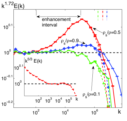
Figure 4: Superfluid (solid lines) and normal fluid (dash lines) compensated energy spectra $k^{1.72}E(k)$; the compensation factor is the classical energy spectrum with intermittency correction. Inset: $k^{5/3}E(k)$ for $T=0.9\,T_{\lambda}$. Shell model simulation of the HVBK model at $T/T_{\lambda}=0.99$ K (green), 0.9 (red) and 0.9 (blue), corresponding to $\rho_{\text{s}}/\rho=0.1\,,\ 0.5\,,$ and 0.9 respectively Boue:PRL2013 . The vertical dash lines indicate $k_{\ell}\equiv 1/\ell$.

VII Models: the Kelvin wave range

Now we come to the more complicated and more intensively discussed aspect of the superfluid energy spectrum: what happens for $k\ell\gg 1$, where the quantisation of vortex lines becomes important. This range acquires great importance at low temperatures, typically below 1 K in ⁴He, and is relevant to turbulence decay experiments. Here we shall describe only the basic ideas, avoiding the most debated details.

For $k\ell\gg 1$ we neglect the interaction between separate vortex lines (besides the small regions around vortex reconnection events, which will be discussed later). Under this reasonable assumption, at large $k$ superfluid turbulence can be considered as a system of Kelvin waves (helix-like deformation of vortex lines) with different wavevectors interacting with each other on the same vortex. The prediction that this interaction results in turbulent energy transfer toward large $k$ Svi95 was confirmed by numerical simulations in which energy was pumped into Kelvin waves at intervortex scales by vortex reconnections Carlo2 or simply by exciting the vortex lines Tsubota3 . The first analytical theory of Kelvin wave turbulence (propagating along a straight vortex line and in the limit of small amplitude compared to wavelength) was proposed by Kozik and Svistunov KS (KS), who showed that the leading interaction is a six-wave scattering process (three incoming waves and three outgoing waves). Under the additional assumption of locality of the interaction (that only compatible wave-vectors contribute to most of the energy transfer) KS found that (using the same normalisation of other hydrodynamic spectra such as Eqs. (3)) the energy spectrum of Kelvin waves is
$\displaystyle E^{{}^{\text{KS}}}_{\scriptscriptstyle\rm{KW}}(k)\simeq\Lambda\,\varepsilon^{1/5}_{\scriptscriptstyle\rm{KW}}\kappa^{7/5}\,\ell^{-8/5}k^{-7/5},\ \qquad\mbox{(KS spectrum).}$
Here $\Lambda\equiv\ln(\ell/\xi)\simeq 12$ or $15$ in typical ⁴He and ³He experiments, and $\varepsilon_{\scriptscriptstyle\rm{KW}}$ is the energy flux in three dimensional ${\bf{k}}$-space.

Later L’vov-Nazarenko (LN) LN criticised the KS assumption of locality and concluded that the leading contribution to the energy transfer comes from a six waves scattering in which two wave vectors (from the same side) have wavenumbers of the order of $1/\ell$. LN concluded that the spectrum is

$$E^{{}^{\text{LN}}}_{\scriptscriptstyle\rm{LN}}(k)\simeq\Lambda\,\varepsilon^{1/3}_{\scriptscriptstyle\rm{KW}}\kappa\,\ell^{-4/3}k^{-5/3},\ \ \mbox{(LN spectrum).}\\$$ (13)

This KS vs LN controversy triggered an intensive debate (see e.g. Refs LN-debate1 ; LN-debate2 ; LN-debate3 ; KS-debate ; Sonin ; LN-Sonin ), which is outside the scope of this article. We only mention that the three–dimensional energy spectrum $E_{KW}(k)$ can be related to the one–dimensional amplitude spectrum $A_{KW}(k)$ by $E_{KW}(k)\sim\hbar\omega n$ where $\omega(k)\sim k^{2}$ is the angular frequency of a Kelvin wave of wavenumber $k$, $\hbar\omega$ the energy of one quantum, and $n\sim A_{KW}$ the number of quanta; therefore, in terms of the Kelvin waves amplitude spectrum (which is often reported in the literature and can be numerically computed), the two predictions are respectively $A_{KW}^{KS}\sim k^{-17/5}=k^{-3.40}$ (KS) and $A_{KW}^{LN}\sim k^{-11/3}=k^{-3.67}$ (LN). The two predicted exponents (-3.40 and -3.67) are very close to each other; indeed VFM simulations Carlo4 could not distinguish them (probably because the numerics were not in the sufficiently weak regime of the theory in terms of ratio of amplitude to wavelength). Nevertheless, more recent GPE simulations by Krstulovic Krs based on long time integration of Eq. (7) and averaged over initial conditions (slightly deviating from a straight line) support the LN spectrum (13).

At finite temperature, it was shown in Ref. BoueLvovProcaccia:EPL2012 that the Kelvin wave spectrum (13) is suppressed by mutual friction for $k>k_{*}$, reaching core scale ($k_{*}\xi\approx 1$) at $T\simeq 0.07\,$K and fully disappears at $T\simeq 1\,$K, when $k_{*}\ell\approx 1$.

VIII Models: near the intervortex scale.

The region of the spectrum near the intervortex scale $k\ell\approx 1$ is difficult because both eddy-type motions and Kelvin waves are important, and the discreteness of the superfluid vorticity prevents direct application of the tools of classical hydrodynamic. Nevertheless, some progress can be made: Sect. VIII.1 presents a differential model for the $T\to 0$ limit LNR-2 , and Sect. VIII.2 describes a complementary truncated HVBK model Salort-2011 designed for the $T>1~{}\rm K$ temperature range.

VIII.1 Differential model of ⁴He at zero temperature

The description of superfluid turbulence for $k\ell\approx 1$ is more complicated than $k\ell\gg 1$ because there are no well justified theoretical approaches (like in the problem of Kelvin wave turbulence at $k\ell\gg 1$) or even commonly accepted uncontrolled closure approximations. Nevertheless, there some qualitative predictions can be tested numerically and experimentally, at least in the zero temperature limit.

Comparison LNR-1 of the hydrodynamic spectrum (3) with the Kelvin wave spectrum at $T=0$ suggests that the one dimensional nonlinear transfer mechanisms among weakly nonlinear Kelvin waves on individual vortex lines is less efficient than the three–dimensional, strongly nonlinear eddy-eddy energy transfer. The consequence is an energy cascade stagnation at the crossover between the collective eddy-dominated scales and the single vortex wave-dominated scales. Ref. LNR-2 argued that the superfluid energy spectrum $E(k)$ at $k\ell\approx 1$ should be a mixture of three–dimensional hydrodynamics modes and one–dimensional Kelvin waves motions; the corresponding spectra should be

$$E^{{}^{\text{HD}}}\!(k)\equiv g(k\ell)E(k)\,,\quad E^{{}^{\text{KW}}}\!(k)\equiv[1-g(k\ell)]E(k)\ .$$

Here

$$g(x)\simeq\big{[}1+x^{2}\exp(x)/4\pi(1+x)\big{]}^{-1}$$

is the“blending” function which was found LNR-2 by calculating the energies of correlated and uncorrelated motions produced by a system of $\ell$-spaced wavy vortex lines.

The total energy flux, $\varepsilon(k)$ arising from hydrodynamic and Kelvin-wave contributions, was modelled LNR-2 by dimensional reasoning in the differential approximation, similar to Eq. (4): for $k\to 0$ the energy flux is purely hydrodynamic and $E(k)$ is given by Eq. (5), while for $k\to\infty$ it is purely supported by Kelvin waves and $E(k)$ is given by Eq. (13). This approach leads to the ordinary differential equation $\varepsilon(k)=$ constant, which was solved numerically. The predicted energy spectra $E(k)$ for different values of $\Lambda$ are shown in Fig. 3C, exhibit a bottleneck energy accumulation $E(k)\propto k^{2}$ in agreement with Eq. (5).

VIII.2 Truncated HVBK model of ⁴He at finite temperature

Recently a model Salort-2011 has been proposed that accounts for the fact that (according to numerical evidence Schwarz1988 ; Mineda:JLTP2012 ; Kivotides-2011 and analytical estimates Samuels1999 ; Vinen:2002 ; BoueLvovProcaccia:EPL2012 ) small scales excitations ($R<\ell$), such as Kelvin waves and isolated rings, are fully damped for $T\gtrsim 1\,$K. Thus, at these temperatures, the energy flux $\varepsilon_{s}(k)$ should be very small at scales $k\gtrsim k_{\ell}$. The idea Salort-2011 was to use the HVBK Eqs. (9) but truncating the superfluid beyond a cutoff wavenumber $k_{\ell^{\star}}=\beta k_{\ell}$, where $\beta$ is a fitting parameter of order one. Obviously, a limitation of this model is the abruptness of the truncation (a more refined model could incorporate a smoother closure which accounts for the dissipation associated with vortex reconnections and the difference between ${\cal L}$ and $|\omega_{s}|/\kappa$).

Direct numerical simulations of this truncated HVBK model for temperatures $1~{}\rm K<T<T_{\lambda}$ with $\beta=0.5$ confirmed the KO–41 scaling of the two locked fluids in the range $k_{D}\ll k<k_{\text{meso}}$ (see Fig. 3A). At smaller scales, an intermediate (meso) regime $k_{\text{meso}}<k<k_{\ell}$ was found that expands as the temperature is lowered Salort-2011 . Apparently, superfluid energy, cascading from larger length scales, accumulates beyond $k_{\text{meso}}$. At the lowest temperatures, this energy appears to thermalize, approaching equipartition with $E_{s}(k)\propto k^{2}$, as shown by the red curve of Fig. 3A. The process saturates when the friction coupling with the normal fluid becomes strong enough to balance the incoming energy flux $\varepsilon(k_{\text{meso}})$. In physical space, this mesoscale thermalization should manifest itself as a randomisation of the vortex tangle. The effect is found to be strongly temperature dependentRoche:EC13 : $k_{\text{meso}}\propto k_{\ell}\sqrt{\rho_{\text{n}}/\rho}$.

The truncated hydrodynamic model reproduces the decreasing spectrum of the vortex line density fluctuations at small $k$ and reduces to the classical spectrum in the $T\rightarrow T_{\lambda}$ limit. This accumulation of thermalized superfluid excitations at small scales and finite temperature was predicted by an earlier model developed to interpret vortex line density spectra Roche-2008 .

IX Conclusions

We conclude that, at large hydrodynamic scales $k_{D}\ll k\ll k_{\ell}$, the evidence for the KO–41 $k^{-5/3}$ scaling of the superfluid energy spectrum which arises from experiments, numerical simulations and theory (across all models used) is strong and consistent, and appears to be independent of temperature (including the limit of zero temperature in the absence of the normal fluid Nore ; Kobayashi ; Araki ; Baggaley-structures ). This direct spectral evidence is also fully consistent with an indirect body of evidence arising from measurements of the kinetic energy dissipation (Walstrom1988a ; Rousset:Pipe1994 ; Abid1998 ; Fuzier:2001p235 ; Salort-2010 ) and vortex line density decay Skrbek2001 ; Niemela:2005p260 in turbulent helium flows. The main open issue is the existence of vortex bundles Baggaley-structures ; Sherwin-2012 predicted by the VFM, for which there is no direct experimental observation yet. Intermittency effects, predicted by shell models Boue:PRL2013 , also await for experimental evidence.

What happens at mesoscales just above $k\approx k_{\ell}$ is less understood. The differential model (at $T=0$, Sect. VIII.1) and the truncated HVBK model (at finite $T$, Sec. VIII.2), predict an upturning of the spectrum (temperature-dependent for the latter model) in this region of $k$-space. If confirmed by the experiments and the VFM model, this would signify the striking appearance of quantum effects at scales larger than $\ell$. Further insight could arise from better understanding of fluctuations of the vortex line density. It is worth noticing that similar macroscopic manifestation of the singular nature of the superfluid vorticity was also predicted for the pressure spectrum Vassilicos-pressure .

At length scales of the order of $\ell$ and less than $\ell$ the situation is even less clear. This regime is very important at the lowest temperatures, where the Kelvin waves are not damped, and energy is transferred from the eddy–dominated, three–dimensional Kolmogorov-Richardson cascade into a Kelvin wave cascade on individual vortex lines, until the wavenumber is large enough that energy is radiated as sound. The main open issues which call for better understanding concern the cross–over and more elaborated description of the bottleneck energy accumulation around $\ell$ in the wide temperature range from 0 to about $T_{\lambda}$ and the role of vortex reconnections in the strong regime (large Kelvin wave amplitudes compared to wavelength) of the cascade. At the moment, there is much debate on these problems but no direct experimental evidence for these effects. It is however encouraging that the most recent GPE simulations Krs in the weak regime (small amplitude compared to wavelength) seem to agree with theoretical predictions.

- (1) A.F. Annett (2004) Superconductivity, superfluids and condensates (Oxford University Press, Oxford).
- (2) L. Skrbek and K.R. Sreenivasan (2012), Developed quantum turbulence and its decay, Phys. Fluids (24): 011301.
- (3) C.F. Barenghi, S. Hulton and D.C. Samuels (2002), Polarization of superfluid turbulence, Phys. Rev. Lett. (89): 275301.
- (4) A.W. Baggaley, J. Laurie, and C.F. Barenghi (2012), Vortex-density fluctuations, energy spectra, and vortical regions in superfluid turbulence, Phys. Rev. Lett. (109): 205304.
- (5) R.J. Donnelly (1991) Quantised Vortices In Helium II (Cambridge University Press, Cambridge, UK).
- (6) C.F. Barenghi, R.J. Donnelly, and W.F. Vinen (1982), Friction on quantized vortices in helium II J. Low Temp. Phys. (52): 189–247.
- (7) R.J. Donnelly and C.F. Barenghi (1998), The observed properties of liquid helium at the saturated vapor pressure, J. Phys. Chem. (6): 1217–1274.
- (8) C. Leith (167), Diffusion approximation to inertial energy transfer in isotropic turbulence, Phys. Fluids (10): 1409–1416.
- (9) C. Connaughton and S. Nazarenko (2004), Warm Cascades and Anomalous Scaling in a Diffusion Model of Turbulence, Phys. Rev. Lett. (92): 044501.
- (10) U. Frisch (1995), Turbulence. The legacy of A.N. Kolmogorov (Cambridge University press, Cambridge, UK).
- (11) A.W. Baggaley, C.F. Barenghi, A. Shukurov, and Y.A. Sergeev (2012), Coherent vortex structures in quantum turbulence, Europhys. Lett. (98): 26002.
- (12) W.F. Vinen (2001), Decay of superfluid turbulence at very low temperature: the radiation of sound from a Kelvin wave on a quantized vortex, Phys. Rev. B (64): 134520.
- (13) S.N. Fisher (2008), Turbulence experiments in superfluid 3He at very low temperatures, in Vortices and Turbulence at Very Low Temperatures, edited by C.F. Barenghi and Y.A. Sergeev, CISM Courses and Lectures, vol. 501, Springer Verlag (2008), 157–257.
- (14) A.W. Baggaley, L.K. Sherwin, C.F. Barenghi, and Y.A. Sergeev (2012), Thermally and mechanically driven quantum turbulence in helium II, Phys. Rev. B (86): 104501.
- (15) S. K. Nemirovskii (2013), Quantum turbulence: Theoretical and numerical problems Physics Reports, (524): 85–120.
- (16) J. Maurer, and P. Tabeling (1998), Local investigation of superfluid turbulence, Europhys. Lett. (43): 29–34.
- (17) D. Schmoranzer, M. Rotter, J. Sebek, and L. Skrbek (2009), Experimental setup for probing a von Karman type flow of normal and superfluid helium, Experimental Fluid Mechanics 2009, Proceedings of the International Conference, 304
- (18) B. Rousset et al., The SHREK superfluid Von Karman flow experiment, Proc. of CEC/ICMC, Anchorage USA, June 2013
- (19) J. Salort, B. Chabaud, Lévêque E. and P.-E. Roche (2012), Energy cascade and the four-fifths law in superfluid turbulence, Europhys. Lett. (97): 34006.
- (20) P.E. Roche, P. Diribarne, T. Didelot, O. Francais, L. Rousseau, and H. Willaime (2007), Vortex density spectrum of quantum turbulence, Europhys. Lett. (77): 66002.
- (21) J. Salort J, et al. (2010), Turbulent velocity spectra in superfluid flows, Phys. Fluids (22): 125102.
- (22) J. Salort, P.-E. Roche and E. Lévêque (2011), Mesoscale Equipartition of kinetic energy in Quantum Turbulence, Europhys. Lett. (94): 24001.
- (23) J. Salort, B. Chabaud, E. Lévêque, and P.-E. Roche (2011). Investigation of intermittency in superfluid turbulence. In J. Phys.: Conf. Ser., volume 318 of Proceedings of the 13th EUROMECH European Turbulence Conference, Sept 12-15, 2011, Warsaw, page 042014. IOP Publishing.
- (24) J. Salort, A. Monfardini, and P.-E. Roche (2012), Cantilever anemometer based on a superconducting micro-resonator: Application to superfluid turbulence, Rev. Sci. Instrum. (83): 125002.
- (25) S.A. Vitiello, L. Reatto, G.V. Chester, and M.H. Kalos (1996), Vortex line in superfluid 4He: A variational Monte Carlo calculation, Phys. Rev. B (54): 1205–1212.
- (26) K.W. Schwarz (1988), Three-dimensional vortex dynamics in superfluid 4He: Homogeneous superfluid turbulence, Phys. Rev. B (38): 2398–2417.
- (27) P.G. Saffman (1992), Vortex Dynamics (Cambridge University Press, Cambridge, UK).
- (28) A.W. Baggaley and C.F. Barenghi (2012), Tree method for quantum vortex dynamics, J. Low Temp. Phys. (66): 3–20.
- (29) A.W. Baggaley (2012), The sensitivity of the vortex filament method to different reconnections models, J. Low Temp. Phys. (68): 18.
- (30) S. Zuccher, M. Caliari, and C.F. Barenghi (2012), Quantum vortex reconnections, Phys. Fluids (24): 125108.
- (31) D. Kivotides, C.F. Barenghi, and D.C. Samuels (2000), Triple vortex ring structure in superfluid helium II, Science (290): 777–779.
- (32) D. Kivotides (2011), Spreading of superfluid vorticity clouds in normal-fluid turbulence, J. Fluid Mech. (668): 58–75.
- (33) H.E. Hall and W.F. Vinen (1956), The rotation of liquid helium II. II. The theory of mutual friction in uniformly rotating helium II. Proc. Roy. Soc. London A (238): 215–234.
- (34) R.N. Hills and P.H. Roberts (1977), Superfluid mechanics for a high density of vortex lines, Arch. Rat. Mech. Anal. (66): 43–71.
- (35) C.F. Barenghi (1992), Vortices and the Couette flow of helium II, Phys. Rev. B (45): 2290–2293.
- (36) K.L. Henderson, C.F. Barenghi and C.A. Jones (1995), Nonlinear Taylor Couette flow of helium II, J. Fluid Mech. (283): 329–340.
- (37) C. Nore, M. Abid, and M.E. Brachet (1997), Kolmogorov turbulence in low temperature superflows, Phys. Rev. Lett. (78): 3896–3899.
- (38) M. Kobayashi, and M. Tsubota (2005), Kolmogorov spectrum of superfluid turbulence: numerical analysis of the Gross-Pitaevskii equation with a small-scale dissipation, Phys. Rev. Lett. (94): 065302.
- (39) N. Sasa, T. Kano, M. Machida, V. S. L’vov, O. Rudenko and M. Tsubota (2011), Energy spectra of quantum turbulence: Large-scale simulation and modelling, Phys. Rev. B (84): 054525.
- (40) V. S. L’vov, S. V. Nazarenko, O. Rudenko (2008), Gradual eddy-wave crossover in superfluid turbulence, J. Low Temp. Phys. (153): 140–161.
- (41) T. Araki, M. Tsubota, and S.K. Nemirovskii (2002), Energy Spectrum of Superfluid Turbulence with No Normal-Fluid Component, Phys. Rev. Lett. (89): 145301.
- (42) M. Tsubota and M. Kobayashi (2009), Energy spectra of quantum turbulence, in Progress of Low Temperature Physics, 1–43, ed. by M. Tsubota and W.P. Halperin, Elsevier.
- (43) N. P. Proukakis and B. Jackson (2008), Finite-temperature models of Bose-Einstein condensation, J Phys B-At Mol Opt 41 (2008): 203002.
- (44) M. E. Brachet (2012), Gross-Pitaevskii description of superfluid dynamics at finite temperature: A short review of recent results, C. R. Physique (13): 954.
- (45) A.J. Allen, E. Zaremba, C.F. Barenghi, and N.P. Proukakis (2013), Observable vortex properties in finite-temperature Bose gases Phys. Rev. A (87): 013630.
- (46) G. Krstulovic and M. Brachet (2011), Anomalous vortex-ring velocities induced by thermally excited Kelvin waves and counterflow effects in superfluids. Phys. Rev. B (83): 132506.
- (47) R.G.K.M. Aarts, and A.T.A.M. de Waele (1994), Numerical investigation of the flow properties of He II, Phys. Rev. B (50) 10069–10079.
- (48) D. Kivotides, C.J. Vassilicos, D.C. Samuels, and C.F. Barenghi (2002), Velocity spectra of superfluid turbulence, Europhys. Lett. (57): 845–851.
- (49) D.R. Osborne, J.C. Vassilicos, K. Sung, and J.D. Haigh (2006), Fundamentals of pair diffusion in kinematic simulations of turbulence, Phys. Rev. E (74): 036309.
- (50) K. Morris, J. Koplik, and D.W.I. Rouson (2008), Vortex locking in direct numerical simulations of quantum turbulence, Phys. Rev. Lett. (101): 015301.
- (51) D. Kivotides (2006), Coherent structure formation in turbulent thermal superfluids, Phys. Rev. Lett. (96): 175301.
- (52) V. S. L’vov, S. V. Nazarenko, O. Rudenko (2007), Bottleneck crossover between classical and quantum superfluid turbulence, Phys. Rev. B 76, 024520.
- (53) H. Adachi, S. Fujiyama, and M. Tsubota (2010), Steady state counterflow turbulence: simulation of vortex filaments using the full Biot-Savart law. Phys. Rev. B (81): 104511.
- (54) P.E. Roche, and C.F. Barenghi (2008), Vortex spectrum in superfluid turbulence: interpretation of a recent experiment, Europhys. Lett. (81): 36002.
- (55) L. Merahi, P. Sagaut, and Z. Abidat (2006), A closed differential model for large-scale motion in HVBK fluids, Europhys. Lett. (75): 757.
- (56) P.-E. Roche, C. F. Barenghi, and E. Lévêque (2009), Quantum turbulence at finite temperature: the two-fluids cascade, Europhys. Lett. (87): 54006.
- (57) J. Tchoufag and P. Sagaut (2010), Eddy damped quasi normal Markovian simulations of superfluid turbulence in helium II , Phys. Fluids, (22): 125103.
- (58) D. H. Wacks and C. F. Barenghi (2011), Shell model of superfluid turbulence, Phys. Rev. B (84): 184505.
- (59) L. Boué, V. L’vov, A. Pomyalov, and I. Procaccia (2013)r,. Enhancement of intermittency in superfluid turbulence. Phys. Rev. Lett. (110): 014502.
- (60) L. Boué, V. L’vov, A. Pomyalov, and I. Procaccia (2012)r,. Energy spectra of superfluid turbulence in 3He Phys. Rev.B (85): 104502.
- (61) V. S. L’vov, S. V. Nazarenko, G. E. Volovik (2004), Energy spectra of developed superfluid turbulence, JETP Letters (80) 479.
- (62) L. Boué, V.S. L’vov, A. Pomyalov, and I. Procaccia (2012), Energy spectra of superfluid turbulence in 3He Phys. Rev. B (85): 104502.
- (63) V. S. L’vov, S. V. Nazarenko, L. Skrbek (2006), Energy Spectra of Developed Turbulence in Helium Superfluids, J. Low Temp. Phys. (145): 125.
- (64) B. V. Svistunov (1995), Superfluid turbulence in the low-temperature limit, Phys. Rev. B (52): 3647.
- (65) D. Kivotides, J.C. Vassilicos, D.C. Samuels, and C.F. Barenghi (2001), Kelvin Waves Cascade in Superfluid Turbulence, Phys. Rev. Lett. (86): 3080.
- (66) W. F. Vinen, M. Tsubota, and A. Mitani (2003), Kelvin-Wave Cascade on a Vortex in Superfluid 4He at a Very Low Temperature, Phys. Rev. Lett. (91): 135301.
- (67) E. Kozik, B.V. Svistunov (2004), Phys. Rev. Lett. (92): 035301.
- (68) V.S. L’vov, S. Nazarenko (2010), Spectrum of Kelvin-wave turbulence in superfluids Pisma v ZhETFf (91): 464.
- (69) J. Laurie, V.S. L’vov, S. Nazarenko, O. Rudenko (2010), Interaction of Kelvin waves and nonlocality of energy transfer in superfluids, Phys. Rev. B. (81): 104526.
- (70) V.V. Lebedev, V.S. L’vov (2010), Symmetries and interaction coefficient of Kelvin waves J. Low Temp. Phys, (161): 548–554.
- (71) V.V. Lebedev, V.S. L’vov, S.V. Nazarenko (2010), Reply: On role of symmetries in Kelvin wave turbulence J. Low Temp. Phys, (161): 606–610.
- (72) E. Kozik, B.V. Svistunov (2010), Geometric symmetries in superfluid vortex dynamics, Phys. Rev. B (82):(R) 140510.
- (73) E.B. Sonin (2012), Symmetry of Kelvin-wave dynamics and the Kelvin-wave cascade in the T=0 superfluid turbulence, Phys. Rev. B (85): 104516.
- (74) V.S. L’vov, S.V. Nazarenko (2012), Comment on Symmetry of Kelvin-wave dynamics and the Kelvin-wave cascade in the T=0 superfluid turbulence, Phys. Rev. B (86): 226501
- (75) A.W. Baggaley and C.F. Barenghi (2011), Spectrum of turbulent Kelvin-waves cascade in superfluid helium, Phys. Rev. B (83): 134509.
- (76) G. Krstulovic (2012), Kelvin-wave cascade and dissipation in low-temperature superfluid vortices Phys. Rev. E (86): 055301.
- (77) L. Boué, V. L’vov, and I. Procaccia (2012). Temperature suppression of Kelvin-wave turbulence in superfluids, Europhys. Lett. (99): 46003.
- (78) Y. Mineda, M. Tsubota, and W. Vinen (2012). Decay of counterflow quantum turbulence in superfluid 4He, J. Low Temp. Phys. 1 10.1007/s10909-012-0800-7
- (79) D. C. Samuels and D. Kivotides (1999), A damping length scale for superfluid turbulence Phys. Rev. Lett. (83): 5306.
- (80) W. F. Vinen and J. J. Niemela (2002), Quantum turbulence, J. Low Temp. Phys. (128): 167.
- (81) P.-E. Roche (2013), Energy spectra and characteristic scales of quantum turbulence investigated by numerical simulations of the two-fluid model, To appear in the Proc. of the 14th EUROMECH European Turbulence Conference, Sept 1-4, 2013, Lyon.
- (82) D. Kivotides, J.C. Vassilicos, C.F. Barenghi, M.A.I. Khan, and D.C. Samuels (2001), Quantum signature of superfluid turbulence Phys. Rev. Lett. (87): 275302.
- (83) LK Sherwin, AW Baggaley and CF Barenghi, in preparation
- (84) P. Walstrom, J. Weisend, J. Maddocks, and S. Van Sciver (1988) Turbulent flow pressure drop in various He II transfer system components. Cryogenics (28):101
- (85) B. Rousset, G. Claudet, A. Gauthier, P. Seyfert, A. Martinez, P. Lebrun, M. Marquet, and R. van Weelderen (1994) Pressure drop and transient heat transport in forced flow single phase helium II at high Reynolds numbers. Cryogenics (34):317
- (86) M. Abid, M. E. Brachet, J. Maurer, C. Nore, and P. Tabeling (1998) Experimental and numerical investigations of low-temperature superfluid turbulence Eur. J. Mech B-Fluid (17):665
- (87) S. Fuzier, B. Baudouy, and S. W. Van Sciver (2001) Steady-state pressure drop and heat transfer in He II forced flow at high Reynolds number Cryogenics (41):453
- (88) L. Skrbek, J. J. Niemela, and K. R. Sreenivasan (2001) Energy spectrum of grid-generated HeII turbulence Phys. Rev. E, (64):067301
- (89) J. Niemela, K. Sreenivasan, and R. Donnelly (2005) Grid generated turbulence in helium II J. Low Temp. Phys. (138):537