Bright solitons from the nonpolynomial Schrödinger equation
with inhomogeneous defocusing nonlinearities

Abstract

Extending the recent work on models with spatially nonuniform nonlinearities, we study bright solitons generated by the nonpolynomial self-defocusing (SDF) nonlinearity in the framework of the one-dimensional (1D) Muñoz-Mateo - Delgado (MM-D) equation (the 1D reduction of the Gross-Pitaevskii equation with the SDF nonlinearity), with the local strength of the nonlinearity growing at $|x|\rightarrow\infty$ faster than $|x|$. We produce numerical solutions and analytical ones, obtained by means of the Thomas-Fermi approximation (TFA), for nodeless ground states, and for excited modes with $\ 1$, $2$, $3,$ and $4$ nodes, in two versions of the model, with steep (exponential) and mild (algebraic) nonlinear-modulation profiles. In both cases, the ground states and the single-node ones are completely stable, while the stability of the higher-order modes depends on their norm (in the case of the algebraic modulation, they are fully unstable). Unstable states spontaneously evolve into their stable lower-order counterparts.

Introduction - The experimental realization of the Bose-Einstein condensates (BECs) of dilute atomic gases AndersonSCi95 ; BradleyPRL95 ; DavisPRL95 allows the investigation of a great many of fascinating phenomena, such as the Anderson localization of matter waves BillyNAT08 ; RoatiNAT08 , production of bright KhaykovichSCi02 ; StreckerNAT02 ; Rb85 ; Cornish and dark solitons BurgerPRL99 , dark-bright complexes dark-bright , vortices MatthewsPRL99 and vortex-antivortex dipoles Anderson ; Hall ; Bagnato ; dipole , persistent flows in the toroidal geometry flow ; flow2 , skyrmions skyrmion , emulation of gauge fields gauge and spin-orbit coupling SO , quantum Newton’s cradles cradle , etc. This subject has been greatly upheld by the use of the Feshbach-resonance (FR) technique, i.e., the control of the strength of the inter-atomic interactions by externally applied fields InouyeNAT98 ; CourteillePRL98 ; RobertsPRL98 , which opens the possibility to implement sophisticated nonlinear patterns. In particular, the management of localized solutions of the Gross-Pitaevskii equation (GPE) GPE by means of the spatially inhomogeneous nonlinearity, which may be created by external nonuniform fields that induce the corresponding FR landscape, has attracted a great deal of interest in theoretical studies Malomed06 ; KartashovRMP11 ; BBPRL08 ; SalasnichPRA09 ; AvelarPRE09 ; CardosoNA10 ; AvelarPRE10 ; CardosoPLA10 ; CardosoPLA10-2 ; CardosoPRE12 .

In this vein, the existence of bright solitons in systems with purely repulsive, alias self-defocusing (SDF) nonlinearity, in the absence of external linear potentials, was recently predicted BorovkovaPRE11 . This result is intriguing because the existence of such solutions, supported by SDF-only nonlinearities, without the help of a linear potential, was commonly considered impossible. In the setting introduced in Ref. BorovkovaPRE11 , the system is described by a nonlinear Schrödinger (NLS) equation with the SDF cubic term, whose strength increases in space rapidly enough towards the periphery. The discovery of bright solitons in this setting has ushered studies of solitary modes in other models with spatially growing repulsive nonlinearities, both local BorovkovaOL11 ; KartashovOL11 ; Zeng12 ; LobanovOL12 ; KartashovOL12 ; Young-SPRA13 and nonlocal He . More specifically, in Ref. BorovkovaOL11 it was demonstrated that spatially inhomogeneous defocusing nonlinear landscapes modulated as $1+|r|^{\alpha}$, with $\alpha>D$ in the space of dimension $D$, support stable fundamental and higher-order bright solitons, as well as localized vortices, with algebraically decaying tails. Further, it was shown in Ref. KartashovOL11 that bimodal systems with a similar spatial modulation of the SDF cubic nonlinearity can support stable two-component solitons, with overlapping or separated components. Work Zeng12 addressed the possibility of supporting stable bright solitons in 1D and 2D media by the SDF quintic term with a spatially growing coefficient. In work LobanovOL12 , it was predicted that a practically relevant setting, in the form of a photonic- crystal fiber whose strands are filled by an SDF nonlinear medium, gives rise to stable bright solitons and vortices. Asymmetric solitons and domain-wall patterns, supported by inhomogeneous defocusing nonlinearity were reported in Ref. KartashovOL12 . Going beyond the limits of BEC and optics, in Ref. Young-SPRA13 self-trapped ground states were predicted to occur in a spin-balanced gas of fermions with repulsion between the spinor components, provided that the repulsion strength grows from the center to periphery, in the combination with the usual harmonic-oscillator trapping potential acting in one or two transverse directions. A very recent result demonstrates that the 2D isotropic or anisotropic nonlinear potential, induced by the strength of the local self-repulsion growing $\sim r^{4}$, can efficiently trap fundamental solitons and vortices with topological charges $1$ and $2$ in the dipolar BEC, with the long-range repulsion between dipoles polarized perpendicular to the system’s confinement plane Kishor .

In the present work, we address the existence of stable bright solitons in the framework of the nonpolynomial Muñoz-Mateo-Delgado (MM-D) equation MateoPRA08 ; Delgado2 (see also Ref. Gerbier ), which is a one-dimensional (1D) reduction of the full three-dimensional GPE for cigar-shaped condensates with repulsive interatomic interactions. Because of the repulsive sign of the intrinsic nonlinearity, the MM-D equation is drastically different from the nonpolynomial NLS equation derived as a result of the dimensional reduction for the self-attractive BEC Luca . In this work, we consider the spatially modulated nonpolynomial nonlinearity whose strength increases rapidly enough towards the periphery, similar to what was originally introduced in Ref. BorovkovaPRE11 for the cubic SDF nonlinearity. Results are obtained analytically by means of the Thomas-Fermi approximation (TFA), and in a numerical form.

The theoretical model - We start with the GPE written in 3D as

$$i\hbar\frac{\partial\Psi}{\partial t}=-\frac{\hbar^{2}}{2m}\nabla^{2}\Psi+g(\mathbf{r})N|\Psi|^{2}\Psi+\frac{1}{2}m\omega_{\perp}^{2}\left(y^{2}+z^{2}\right)\Psi,$$ (1)

where $\Psi(\mathbf{r},t)$ is the mean-field wave function, $\nabla^{2}$ is the Laplacian, $g(\mathbf{r})$ is the spatially-dependent local coefficient of the self-repulsive nonlinearity, $\omega_{\perp}$ is the strength of the harmonic-oscillator (HO) trapping potential applied in the transverse plane, $\left(y,z\right)$, while $m$ and $N$ are the atomic mass and the number of particles, respectively. In Refs. MateoPRA07 and MateoPRA08 it has been shown that the effective 1D equation governing the axial dynamics of cigar-shaped condensates with the repulsive interatomic interactions can be derived as a reduction of the 3D equation (1):

$$i\hbar\frac{\partial\psi}{\partial t}=-\frac{\hbar^{2}}{2m}\frac{\partial^{2}\psi}{\partial x^{2}}+\hbar\omega_{\bot}\sqrt{1+4a(x)N|\psi|^{2}}\psi,$$ (2)

with $a(x)>0$ being the $s$-wave scattering length, whose dependence on axial coordinate $x$ may be imposed by means of the FR management. The corresponding 3D wave function is approximated by the factorized ansatz,$\ \Psi=\psi(x,t)\Phi(\mathrm{r}_{\bot},n_{1}(x,t))$, where $n_{1}$ is the axial density, $n_{1}=N\int\int\mathrm{d}y\mathrm{d}z\mathrm{~{}}|\Psi\left(x,y,z\right)|^{2}$, and $\Phi(\mathrm{r}_{\bot},$$n_{1})$ is the transverse wave function satisfying equation [see Eq. (15) of Ref. MateoPRA08 )]

$$\left(-\frac{1}{2}\overline{\nabla}^{2}+\frac{1}{2}\overline{r}_{\bot}^{2}+4\pi an_{1}|\overline{\Phi}|^{2}\right)\overline{\Phi}=\overline{\mu}_{\bot}\overline{\Phi},$$ (3)

written in scaled variables $\overline{r}_{\bot}=r_{\bot}/a_{\bot}$, $\overline{\Phi}=a_{\bot}\Phi$, and $\overline{\mu}_{\bot}=\mu_{\bot}/\hbar\omega_{\bot}$. Here $\mu_{\bot}=\mu_{\bot}(n_{1})$ is the local chemical potential, and $a_{\bot}=\sqrt{\hbar/m\omega_{\bot}}$ is the confinement length in the transverse direction. Equation (3) admits explicit approximate solutions in the limit cases of $an_{1}\ll 1$ and $an_{1}\gg 1$, treating $\overline{\Phi}$, severally, as the Gaussian ground state of the HO potential, or the TFA wave function MateoPRA08 .

Finally, Eq. (2) is transformed into a scaled form,

$$i\frac{\partial\varphi}{\partial t}=-\frac{1}{2}\frac{\partial^{2}\varphi}{\partial x^{2}}+\sqrt{1+\sigma(x)|\varphi|^{2}}\varphi,$$ (4)

where $\sigma(x)\equiv 4a(x)/a_{\bot}$. Stationary solutions to Eq. (4) with (longitudinal) chemical potential $\mu$ are looked for as usual,

$$\varphi(x,t)=\phi(x)e^{-i\mu t}.$$ (5)

The application of the TFA, which neglects the kinetic-energy term GPE , to Eq. (4) immediately yields

$$\phi_{\mathrm{TFA}}^{2}=\frac{\mu^{2}-1}{\sigma(x)},$$ (6)

provided that the chemical potential takes values $\mu>1$. In the same approximation, the norm (scaled number of atoms) of the condensate is

$$N_{\mathrm{TFA}}=\left(\mu^{2}-1\right)\int_{-\infty}^{+\infty}\frac{dx}{\sigma(x)},$$ (7)

provided that $\sigma(x)$ grows at $|x|\rightarrow\infty$ faster than $|x|$, to secure the convergence of the integral. In fact, the latter condition is the exact one which is necessary and sufficient for the existence of physically relevant self-trapped modes in the MM-D equation.

The results produced by the TFA in the form of Eq. (6) were used as the initial guess for finding numerically exact stationary solutions by means of the well-known method of the imaginary-time integration, in the framework of which the convergence of stationary solutions may be related to their stability against small perturbations in real time Yang10 . As characteristic examples, we use two different axial nonlinearity-modulation profiles,

$$\sigma_{\mathrm{A}}(x)=\cosh^{2}(2x);~{}~{}\sigma_{\mathrm{B}}(x)=1+x^{6},$$ (8)

cf. Refs. BorovkovaPRE11 -Zeng12 . Below, these two profiles are referred to as Cases A and B, respectively.

The stability of the self-trapped modes was investigated in the framework of the linearized equations, taking the perturbed solutions as

$$\varphi=\left\{\phi(x)+\left[v(x)+w(x)\right]e^{\lambda t}+\left[v^{\ast}(x)-w^{\ast}(x)\right]e^{-\lambda^{\ast}t}\right\}e^{i\mu t},$$ (9)

where $v(x)$ and $w(x)$ are small perturbations, and $\lambda$ is the respective eigenvalue. The ensuing linear-stability eigenvalue problem was solved by means of the Fourier Collocation Method, as described in Ref. Yang10 .

First, we have analyzed the stability for the ground-state solutions produced by the TFA (used as the initial guess for the numerical stationary solutions). It has been found that they are stable for all $\mu>1$, see further details below. It is also worthy to note that, as it follows from Eq. (7) and corroborated below by numerical results, the families of the ground-state modes obey the anti-Vakhitov-Kolokolov (anti-VK) criterion, $dN/d\mu>0$, which is a necessary stability condition for localized modes supported by SDF nonlinearities anti (the VK criterion per se, relevant to the usual solitons supported by the self focusing nonlinearity, VakhitovRQE73 ; BergePR98 , has the opposite form, $dN/d\mu<0$).

Numerical Results - The integration in imaginary time was carried out by means of the split-step code, which was composed so as to restore the original norm of the solution at the end of each step of marching forward in imaginary time. The dispersive part of Eq. (4) was handled by means of the Crank-Nicolson algorithm with spatial and temporal steps $\Delta x=0.04$ and $\Delta t=0.001$.

To find higher-order stationary solutions with nodes, the Gram-Schmidt orthogonalization was performed at the end of each time step. The ground-state and higher-order solutions were thus obtained, using the Hermite-Gaussian input profiles of orders $n=0,1,2,3,4.$ To check the correctness of the stationary solutions, we have also reproduced them by means of the standard relaxation method, concluding that the solutions obtained by dint of both techniques were indistinguishable. Finally, the stability was checked via the real-time simulations of the perturbed evolution of input profiles to which random noise was added at the $5\%$ amplitude level, as well as through the computation of the stability eigenvalues for perturbed solution taken as in Eq. (9).

Case A) As said above, the exponential modulation profile of the nonlinearity coefficient, corresponding to $\sigma_{\mathrm{A}}(x)$ in Eq. (8), is suggested by its counterpart that was used with the quintic nonlinearity in Ref. Zeng12 . In Fig. 1(a) we display the relation between the chemical potential $\mu$ and norm $N$ for stationary solutions $\phi_{k}$ of different orders (number of nodes) $k$, obtained with this profile. Typical examples of the stationary modes are shown in panels 1(b-f).

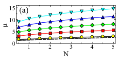
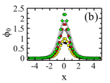
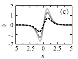
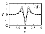
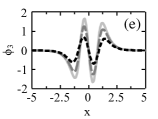
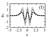
Figure 1: (Color online) The model with the nonlinearity-modulation function $\sigma_{\mathrm{A}}(x)=\cosh^{2}\left(2x\right)$. (a) Chemical potential $\mu$ versus norm $N$ for the ground-state solution, $\phi_{0}$ (the yellow curve with circles), the first excited state, $\phi_{1}$ (the red curve with box-shaped symbols), the second-order mode, $\phi_{2}$ (the green curve with diamond symbols), the third-order mode, $\phi_{3}$ (the blue curve with triangles), and the fourth-order mode, $\phi_{4}$ (the cyan curve with inverted triangles). The dashed line shows the TFA prediction for the ground state, see Eqs. (6) and (7). Profiles of stationary solutions produced by the imaginary-time integration method: $\phi_{0}$ (b), $\phi_{1}$ (c), $\phi_{2}$ (d), $\phi_{3}$ (e), and $\phi_{4}$ (f), with norms $N=1$ (dashed lines), $N=3$ (long-dashed lines), and $N=5$ (solid lines). In panel (b), the corresponding TFA-predicted shapes are shown by chains of circles ($N=1$), boxes ($N=3$), and diamonds ($N=5$).

All the solution branches satisfy the above-mentioned anti-VK criterion. We have checked that, in agreement with this fact, the ground-state modes, $\phi_{0}$, are stable for all $\mu>1$. However, for higher-order modes this criterion is necessary but not sufficient for the stability. We have thus found that the first excited state, $\phi_{1}$, is fully stable, while higher-order ones, $\phi_{2,3,4}$ are stable only in specific regions (we have checked this up to the value of the total norm $N=15$). This trend (the full stability of the ground and first excited states, and partial instability of the higher-order ones) is similar to that featured by the model with the spatially growing local strength of the cubic SDF nonlinearity BorovkovaPRE11 .

Results of the linear-stability analysis, based on Eq. (9), are presented in Fig. 2, which displays the largest real part of the eigenvalue, $\lambda_{R}$, versus the norm for solutions $\phi_{2}$ (a), $\phi_{3}$ (b), and $\phi_{4}$ (c). It is seen that the instability sets in with the increase of the norm. As examples, in Figs. 3 and 4 we show the density profiles, $|\psi(x)|^{2}$, for $N=1$ and $N=5$, respectively, generated in the direct simulations of the perturbed evolution of the input states $\phi_{2}$, $\phi_{3}$, and $\phi_{4}$, with the addition of the $5\%$ random noise. The results agree with the predictions of the linear-stability analysis, cf. Fig. 2.

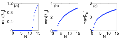
Figure 2: (Color online) The model with $\sigma_{\mathrm{A}}(x)=\cosh^{2}\left(2x\right)$. The largest instability growth rate, $\lambda_{R}$, produced by the linear-stability analysis based on Eq. (9), versus the norm of the unperturbed solution, for the second-order mode, $\phi_{2}$ (a), third-order model, $\phi_{3}$ (b), and the fourth-order one, $\phi_{4}$ (c).

Direct simulations confirm the predictions of the linear-stability analysis, as shown in Figs. 3 and 4. All unstable higher-order modes (at least, up to norm $N=15$) are spontaneously transformed into stable modes of lower orders (with fewer nodes). In particular, the unstable $\phi_{4}$ mode in Fig. 4(c) decays into $\phi_{1}$, although mode $\phi_{2}$ is stable here too. In some other cases, the unstable mode decays directly to the ground state, $\phi_{0}$, although the stable $\phi_{1}$ mode exists too.

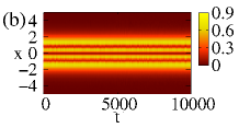
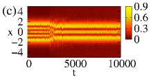
Figure 3: (Color online) The model with $\sigma_{\mathrm{A}}(x)=\cosh^{2}\left(2x\right)$: The real-time evolution of perturbed modes of orders $k=2$ (a), $k=3$ (b), and $k=4$ (c) with norm $N=1$. In panels (a) and (b) the solutions are stable, while in (c) $\phi_{4}$ is unstable, decaying into $\phi_{2}$.

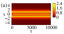
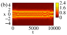
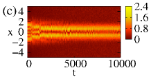
Figure 4: (Color online) The same as in Fig. 3, but for norm $N=5$. The solution is stable in (a), and unstable in (b) and (c).

Case B) The algebraic (mild) modulation of the nonlinearity coefficient is represented by $\sigma_{\mathrm{B}}(x)$ from Eq. (8). For this version of the model, chemical potential $\mu$ is shown, as a function of norm $N$, in Fig. 5(a) for different modes $\phi_{k}$ [the prediction of the TFA for the ground state, given by Eq. (6), in shown by the dashed line].

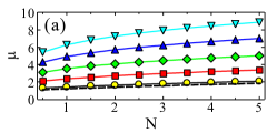
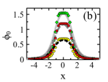
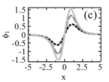
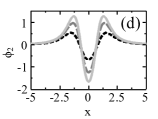
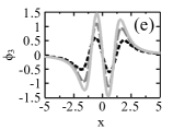
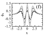
Figure 5: (Color online) The same as in Fig. 1, but for the nonlinearity-modulation function $\sigma_{\mathrm{B}}(x)=1+x^{6}$.

Numerical simulations confirm the stability of all the ground-state solutions, $\phi_{0}$, for all $\mu>1$. However, the stability regions for higher-order modes differ from the version of the model corresponding to $\sigma_{\mathrm{A}}(x)$ in Eq. (8), as concerns instability regions for higher-order modes. In this case too, we have checked the stability for $N\leq 15$, concluding that $\phi_{1}$ is completely stable, while $\phi_{2,3,4}$ are unstable at all values of the norm. Similarly to Case A, but much faster, unstable solutions decay into lower-order stable states, $\phi_{0}$ or $\phi_{1}$. As typical examples, in Fig. 6 we display a stable single-node solution, $\phi_{1}$, and the spontaneous decay of multi-node solutions into lower-order states, for $N=5$. In the model with the modulated local strength of the cubic self-repulsive term, the mild algebraic form of the modulation also gives rise to solitons families which are less stable than their counterparts obtained in the model with the steep exponential modulation, cf. Refs. BorovkovaOL11 and BorovkovaPRE11 .

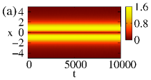
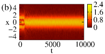
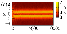
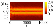
Figure 6: (Color online) The same as in Fig. 4, but for $\sigma_{\mathrm{B}}(x)=1+x^{6}$. (a): The stable evolution of mode $\phi_{1}$. (b), (c), and (d): Unstable evolution of modes $\phi_{2}$, $\phi_{3}$, and $\phi_{4}$, respectively.

Conclusion - We have shown that the MM-D (Muñoz-Mateo - Delgado) equation, which is the 1D nonpolynomial reduction of the 3D GPE with the self-repulsive cubic nonlinearity, supports stable fundamental and higher-order self-trapped modes (“solitons”), provided that the local strength of the nonlinearity grows faster than $|x|$ at $|x|\rightarrow\infty$. We have studied in detail two nonlinearity-modulation patterns, one steep (exponential), and one mild (algebraic). In these models, the ground state (which was approximated analytically by means of the TFA), and the single-node excited state are completely stable, while the stability of higher-order (multi-node) excited modes depends on their norm, and is different in the two models. In direct simulations, the evolution of unstable modes always leads to their spontaneous transformation into stable ones of lower orders.

It may be interesting to extend the analysis for fundamental solitons and solitary vortices in the 2D setting, with the tight confinement acting in the transverse direction, and the nonlinearity strength growing along the radius, $r$, faster than $r^{2}$.

Acknowledgments - W.B.C, A.T.A, and D.B. thank Brazilian agencies, CNPq, CAPES, FAPESP, and Instituto Nacional de Ciência e Tecnologia-Informação Quântica, for partial support. J.Z. acknowledges support from the Natural Science Foundation of China (Project No. 11204151). The work of B.A.M. was supported, in a part, by the German-Israel Foundation (Grant No. I-1024-2.7/2009), and Binational (US-Israel) Science Foundation (Grant No. 2010239).

References

- (1) M. H. Anderson, J. R. Ensher, M. R. Matthews, C. E. Wieman, and E. A. Cornell, Science 269, 198 (1995).
- (2) C. C. Bradley, C. A. Sackett, J. J. Tollett, and R. G. Hulet , Phys. Rev. Lett. 75, 1687 (1995).
- (3) K. B. Davis, M.-O. Mewes, M. R. Andrews, N. J. van Druten, D. S. Durfee, D. M. Kurn, and W. Ketterle , Phys. Rev. Lett. 75, 3969 (1995).
- (4) J. Billy, V. Josse, Z. Zuo, A. Bernard, B. Hambrecht, P. Lugan, D. Clément, L. Sanchez-Palencia, P. Bouyer, and A. Aspect, Nature 453, 891 (2008).
- (5) G. Roati, C. D’Errico, L. Fallani, M. Fattori, C. Fort, M. Zaccanti, G. Modugno, M. Modugno, and M. Inguscio, Nature 453, 895 (2008).
- (6) L. Khaykovich, F. Schreck, G. Ferrari, T. Bourdel, J. Cubizolles, L. D. Carr, Y. Castin, and C. Salomon, Science 296, 1290 (2002).
- (7) K. E. Strecker, G. B. Partridge, A. G. Truscott, and R. G. Hulet, Nature (London) 417, 150 (2002).
- (8) S. L. Cornish, S. T. Thompson, and C. E. Wieman, Phys. Rev. Lett. 96, 170401 (2006).
- (9) A. L. Marchant, T. P. Billam, T. P. Wiles, M. M. H. Yu, S. A. Gardiner, and S. L. Cornish, Nature Commun. 4, 1865 (2013).
- (10) S. Burger, K. Bongs, S. Dettmer, W. Ertmer, K. Sengstock, A. Sanpera, G. V. Shlyapnikov, and M. Lewenstein, Phys. Rev. Lett. 83, 5198 (1999).
- (11) C. Becker, S. Stellmer, P. Soltan-Panahi, S. Dörscher, M. Baumert, E.-M. Richter, J.Kronjäger, K. Bongs, and K. Sengstock, Nature Phys. 4, 496 (2008).
- (12) M. R. Matthews, B. P. Anderson, P. C. Haljan, D. S. Hall, C. E. Wieman, and E. A. Cornell , Phys. Rev. Lett. 83, 2498 (1999).
- (13) T. W. Neely, E. C. Samson, A. S. Bradley, M. J. Davis, and B. P. Anderson, Phys. Rev. Lett. 104, 160401 (2010).
- (14) D. V. Freilich, D. M. Bianchi, A. M. Kaufman, T. K. Langin, and D. S. Hall, Science 329, 1182 (2010).
- (15) J. A. Seman, E. A. L. Henn, M. Haque, R. F. Shiozaki, E. R. F. Ramos, M. Caracanhas, P. Castilho, C. Castelo Branco, P. E. S. Tavares, F. J. Poveda-Cuevas, G. Roati, K. M. F. Magalhães, and V. S. Bagnato, Phys. Rev. A 82, 033616 (2010).
- (16) S. Middelkamp, P. J. Torres, P. G. Kevrekidis, D. J. Frantzeskakis, R. Carretero-González, P. Schmelcher, D. V. Freilich, and D. S. Hall, Phys. Rev. A 84, 011605(R) (2011).
- (17) C. Ryu, M. F. Andersen, P. Cladé, V. Natarajan, K. Helmerson, and W. D. Phillips, Phys. Rev. Lett. 99, 260401 (2007).
- (18) A. Ramanathan, K. C. Wright, S. R. Muniz, M. Zelan, W. T. Hill, C. J. Lobb, K. Helmerson, W. D. Phillips, and G. K. Campbell, Phys. Rev. Lett. 106, 130401 (2011).
- (19) S. Wüester, T. E. Argue, and C. M. Savage, Phys. Rev. A 72, 043616 (2005).
- (20) Y-J. Lin, R. L. Compton, K. Jiménez-García,W. D. Phillips, J. V. Porto and I. B. Spielman, Nature Phys. 7, 531 (2011).
- (21) Y.-J. Lin, K. Jiménez-García, and I. B. Spielman, Nature 471, 83 (2011).
- (22) T. Kinoshita, T. Wenger and D. S. Weiss, Nature 440, 900 (2006).
- (23) S. Inouye, M. R. Andrews, J. Stenger, H.-J. Miesner, D. M. Stamper-Kurn, and W. Ketterle, Nature 392, 151 (1998).
- (24) Ph. Courteille, R. S. Freeland, D. J. Heinzen, F. A. van Abeelen, and B. J. Verhaar, Phys. Rev. Lett. 81, 69 (1998).
- (25) J. L. Roberts, N. R. Claussen, J. P. Burke, Jr., C. H. Greene, E. A. Cornell, and C. E. Wieman, Phys. Rev. Lett. 81, 5109 (1998).
- (26) L. P. Pitaevskii and A. Stringari, Bose-Einstein Condensation (Clarendon Press: Oxford, 2003).
- (27) B. A. Malomed, Soliton Management in Periodic Systems (Springer, New York, 2006).
- (28) Y. V. Kartashov, B. A. Malomed, and L. Torner, Rev. Mod. Phys. 83, 247 (2011).
- (29) J. Belmonte-Beitia, V. M. Pérez-García, V. Vekslerchik, and V. V. Konotop, Phys. Rev. Lett. 100, 164102 (2008).
- (30) L. Salasnich and B. A. Malomed, Phys. Rev. A 79, 053620 (2009).
- (31) A. T. Avelar, D. Bazeia, and W. B. Cardoso, Phys. Rev. E 79, 025602(R) (2009).
- (32) W. B. Cardoso, A. T. Avelar, and D. Bazeia, Nonlin. Anal. RWA 11, 4269 (2010).
- (33) A. T. Avelar, D. Bazeia, and W. B. Cardoso, Phys. Rev. E 82, 057601 (2010).
- (34) W. B. Cardoso, A. T. Avelar, and D. Bazeia, Phys. Lett. A 374, 2640 (2010).
- (35) W. B. Cardoso, A. T. Avelar, D. Bazeia, and M. S. Hussein, Phys. Lett. A 374, 2356 (2010).
- (36) W. B. Cardoso, A. T. Avelar, and D. Bazeia, Phys. Rev. E 86, 027601 (2012).
- (37) O. V. Borovkova, Y. V. Kartashov, L. Torner, and B. A. Malomed, Phys. Rev. E 84, 035602(R) (2011).
- (38) O. V. Borovkova, Y. V. Kartashov, B. A. Malomed, and L. Torner, Opt. Lett. 36, 3088 (2011).
- (39) Y. V. Kartashov, V. A. Vysloukh, L. Torner, and B. A. Malomed, Opt. Lett. 36, 4587 (2011).
- (40) J. Zeng and B. A. Malomed, Phys. Rev. E 86, 036607 (2012).
- (41) V. E. Lobanov, O. V. Borovkova, Y. V. Kartashov, B. A. Malomed, and L. Torner, Opt. Lett. 37, 1799 (2012).
- (42) Y. V. Kartashov, V. E. Lobanov, B. A. Malomed, and L. Torner, Opt. Lett. 37, 5000 (2012).
- (43) L. E. Young-S., L. Salasnich and B. A. Malomed, Phys. Rev. A 87, 043603 (2013).
- (44) Y. He and B. A. Malomed, Phys. Rev. A 87, 053812 (2013).
- (45) R. Kishor Kumar, P. Muruganandam and B. A. Malomed, arXiv:1308.0468; J. Phys. B: At. Mol. Opt. Phys., in press.
- (46) A. Muñoz Mateo and V. Delgado, Phys. Rev. A 77, 013617 (2008).
- (47) A. Muñoz Mateo and V. Delgado, Ann. Phys. (N.Y.) 324, 709 (2009).
- (48) F. Gerbier, Europhys. Lett. 66, 771 (2004).
- (49) L. Salasnich, A. Parola, and L. Reatto, Phys. Rev. A 65, 043614 (2002).
- (50) A. Muñoz-Mateo and V. Delgado, Phys. Rev. A. 74, 065602 (2006); 75, 063610 (2007).
- (51) J. Yang, Nonlinear Waves in Integrable and Nonintegrable Systems (SIAM, Philadelphia, 2010).
- (52) H. Sakaguchi and B. A. Malomed, Phys. Rev. A 81, 013624 (2010).
- (53) M. Vakhitov and A. Kolokolov, Radiophys. Quantum Electron. 16, 783 (1973).
- (54) L. Bergé, Phys. Rep. 303, 259 (1998); E. A. Kuznetsov and F. Dias, ibid. 507, 43 (2011).