Extrapolation of Stationary Random Fields

Abstract

We introduce basic statistical methods for the extrapolation of stationary random fields. For square integrable fields, we set out basics of the kriging extrapolation techniques. For (non–Gaussian) stable fields, which are known to be heavy tailed, we describe further extrapolation methods and discuss their properties. Two of them can be seen as direct generalizations of kriging.

1 Introduction

In this chapter, we consider the problem of extrapolation (prediction) of random fields arising mainly in geosciences, mining, oil exploration, hydrosciences, insurance, etc. It is one of the fundamental tools in geostatistics that provides statistical inference for spatially referenced variables of interest. Examples of such quantities are the amount of rainfall, concentration of minerals and vegetation, soil texture, population density, economic wealth, storm insurance claim amounts, etc.

The origins of geostatistics as a mathematical science can be traced back to the works by B. Mathérn (1960) Matern60 , L. Gandin (1963) Gan63 , G. Matheron (1962-63) Ma62 ; Ma63 . However, the mathematical foundations were already laid in the paper by A.N.Kolmogorov (1941) Kol41 as well as in the book by N.Wiener (1949) Wie49 , where the extrapolation of stationary time series was studied, whereas their practical application is known since 1951 due to mining engineer D. G. Krige Kri51 . Typical practical problems to solve are e.g. plotting the contour concentration map of minerals (interpolation), inference of the the mean areal precipitation and evaluation of accuracy of the estimate from spatial measurements (averaging or generalization), selection of locations of new monitoring points so that the concentration can be evaluated with sufficient accuracy (monitoring network design).

The remainder of this chapter is divided into three sections. Section  2 contains preliminaries about distributional invariance properties and dependence structure of random fields. In Section 3, we concentrate on kriging which is a widely used probabilistic extrapolation technique for the fields with the finite second moment. Section 4 contains recent results on the extrapolation of heavy tailed random fields with infinite variance, namely of stable random fields.

In Sections 2 and 3 we mainly follow the books CD99 ; Cres91 ; BS12 ; Wack03 . Section 4 is based on the paper KSS12 , it also contains some new results for stable fields with the infinite first moment, see Section 4.4.

2 Basics of Random Fields

Let $(\Omega,{\cal{F}},\mathbf{P})$ be a probability space.

Definition 1

A random field $X$ is a random function on $(\Omega,{\cal{F}},\mathbf{P})$ indexed by points of $\mathbb{R}^{d},$ $d\in\mathbb{N}$, i.e. $X$ is a measurable mapping $X:\Omega\times\mathbb{R}^{d}\to\mathbb{R}$.

For an introduction into the theory of random functions see e.g. (BS12, , Chap. 9).

2.1 Random Fields with Invariance Properties

A random field with the finite-dimensional distributions that are invariant with respect to the action of a group $G$ of transformations of $\mathbb{R}^{d}$ is called $G$-invariant in strict sense. In case if this invariance is given only for the first two moments of the field which are assumed to be finite we speak about the $G$–invariance in wide sense. Thus, if $G$ is the group of all translations of $\mathbb{R}^{d}$ then one calls such random fields stationary (in respective sense). For $G$ being the group of rotations $SO_{d}$ one claims the random field to be isotropic. If $G$ is the group of all rigid motions then such field is called motion invariant. The same notions of invariance can be transferred to the increments of random fields. In this case, the stationarity is often called intrinsic. The intrinsic stationarity in wide sense is called intrinsic stationarity of order two. For more details on invariance properties confer (BS12, , Sect. 9.5).

Exercise 1

Show that the expectation (if it exists) of any process ($d=1$) with stationary increments is a linear function, i.e., $\mathbf{E}X(t)=a\cdot t+c$ for all $t\in\mathbb{R}$, $a\in\mathbb{R}$, $c\in\mathbb{R}$.

A popular class of random fields are Gaussian fields.

Definition 2

A random field $X=\{X(t),\;t\in\mathbb{R}^{d}\}$ is Gaussian if all its finite dimensional distributions are Gaussian.

Their use for modelling purposes in applications is explained mainly by the simplicity of their construction and analytic tractability combined with the normal distribution of marginals which describes many real phenomena due to the Central Limit Theorem.

By Kolmogorov’s theorem, the probability law of a Gaussian random field is defined uniquely by its mean value and covariance function; see (BS12, , Sect. 9.2.2) for more details. If the mean value function $\mathbf{E}\,X(t),$ $t\in\mathbb{R}^{d}$ is identically zero we call $X$ to be centered. Without loss of generality we tacitly assume all random fields of this chapter to be centered.

Exercise 2

Show that for Gaussian random fields stationarity (isotropy, motion invariance) in strict sense and stationarity (isotropy, motion invariance) in wide sense are equivalent. In this case we call a Gaussian field just stationary (isotropic, motion invariant).

Examples of Gaussian Random Fields

1. Ornstein-Uhlenbeck Process

A centered Gaussian process $X=\{X(t),\;t\in\mathbb{R}\}$ with the covariance function $\mathbf{E}\left(X(s)X(t)\right)=e^{-|s-t|/2}$, $s,t\in\mathbb{R}$ is called Ornstein-Uhlenbeck Process. Breiman (1968) (Brei68, , p. 350) has shown that $X$ is the only stochastically continuous stationary Markov Gaussian process. Additionally, it has short memory, i.e.,

$$X(t)\stackrel{{\scriptstyle d}}{{=}}e^{-t/2}X(0)+V(t),\quad t>0,$$

where $V(t)$ does not depend on the past $\{X(s),s\leq 0\}$, cf. (Lif12, , Example 2.6, p.11). Defined on $\mathbb{R}_{+}$, $X$ is the strong solution of the Langevin stochastic differential equation

$$dX(t)=-1/2X(t)dt+dW(t)$$

with initial value $X(0)\sim N(0,1)$, where $W=\{W(t),\;t\geq 0\}$ is the standard Wiener process, see e.g. (Bulinski2, , Chapt. 8, Theorem 7). It holds also $X\stackrel{{\scriptstyle d}}{{=}}\left\{e^{-t/2}W\left(e^{\;t}\right),\;t\in\mathbb{R}\right\}$, cf. (Bulinski2, , Chapt. 3, p.107).

2. Gaussian Linear Random Function

A Gaussian linear random function $X=\{X(t),\;t\in l_{2}\}$ is defined by $X(t)=\langle N,t\rangle_{2}$, $t\in l_{2}$, where $N=\{N_{i}\}_{i=1}^{\infty}$ is an i.i.d. sequence of $N(0,1)$-random variables, and $l_{2}$ is the Hilbert space of sequences $t=\{t_{i}\}_{i=1}^{\infty}$ such that $\|t\|^{2}_{2}:=\sum_{i=1}^{\infty}t_{i}^{2}<\infty$ with scalar product $\langle s,t\rangle_{2}=\sum_{i=1}^{\infty}s_{i}t_{i}$, $s,t\in l_{2}$. Since $N$ is not an element of $l_{2}$ a.s., the expression $\langle N,t\rangle_{2}$ is understood formally as the series $\sum_{i=1}^{\infty}N_{i}t_{i}$ which converges in the mean square sense:

$$\mathbf{E}\left|\sum_{i=n}^{m}N_{i}t_{i}\right|^{2}=\sum_{i=n}^{m}t_{i}^{2}\rightarrow 0,\quad n,m\rightarrow\infty.$$

It holds

$$X(t)\sim N(0,\|t\|^{2}_{2}),\quad X(t)-X(s)=X(t-s),\quad\mathbf{E}\left(X(s)X(t)\right)=\langle s,t\rangle_{2},\quad s,t\in l_{2}.$$

Its variogram $\gamma(h):=1/2\cdot\mathbf{E}(X(t+h)-X(t))^{2}$ can be computed as

$$\gamma(h)=\frac{1}{2}\mathbf{E}[X(h)]^{2}=\frac{\|h\|_{2}^{2}}{2},\quad h\in l_{2},$$

see more about variograms in Sect. 2.2. Here we have $\gamma(h)\rightarrow\infty$ as $\|h\|_{2}\rightarrow\infty$. Transferring the notions of stationarity from the index space $\mathbb{R}^{d}$ to $l_{2}$, it is clear that $X$ is intrinsic stationary of order two but not wide sense stationary. Confer IbrRoz for the general theory of Gaussian random functions on Hilbert index spaces.

3. Fractional Brownian Field

A fractional Brownian field $X=\{X(t),\;t\in\mathbb{R}^{d}\}$ is a centered Gaussian field with covariance (see more about covariance in Sect. 2.2)

$$\mathbf{E}(X(s)X(t))=\frac{1}{2}\left(\|s\|^{2H}+\|t\|^{2H}-\|s-t\|^{2H}\right),\quad s,t\in\mathbb{R}^{d}$$

for some $H\in(0,1]$ where $\|\cdot\|$ is the Euclidean norm in $\mathbb{R}^{d}$. Parameter $H$ (often called Hurst index) is responsible for the regularity of the paths of $X$. The greater $H$, the smoother are the paths. For $d=1$, $X$ is called the fractional Brownian motion, including the two–sided Wiener process (defined on the whole $\mathbb{R}$) if $H=1/2$. In the case $d>1$, $H=1/2$ it is called the Brownian Lévy field (see, e.g., (Lif12, , Sect. 2)).

It is easy to check that $X$ is intrinsically stationary of order two and isotropic. Its variogram $\gamma(h)=1/2\cdot\|h\|^{2H}$ is clearly motion invariant. This field is not wide sense stationary as its variance is not constant.

Exercise 3

Show that $X$

1. has stationary increments which are positively correlated for $H\in(1/2,1)$ and negatively correlated for $H\in(0,1/2)$.

2. is $H$–self similar, i.e., $X(\lambda t)\stackrel{{\scriptstyle d}}{{=}}|\lambda|^{H}X(t)$ for all $\lambda\in\mathbb{R}$ and $t\in\mathbb{R}^{d}$.

3. has a version with a.s. Hölder continuous paths of any order $\beta\in(0,H)$.

4. has nowhere differentiable paths for any $H\in(0,1)$.

5. is a linear process for $d=H=1$, i.e., $X(t)\stackrel{{\scriptstyle d}}{{=}}tX_{0}$, $t\in\mathbb{R}$ for a random variable $X_{0}\sim N(0,1)$.

Examples of Non-Gaussian Random Fields

1. Lévy Process with Finite Second Moments

Let $X=\{X(t),\;t\geq 0\}$ be a Lévy process with finite second moments. It is usually defined via the Lévy–Khinchin triplet coding its jump structure, see e.g. Sat99 . It is clear that $X$ is intrinsic stationary of order two, but not wide sense stationary. For each of these processes one can calculate the variance of increments and the variogram, for example,

$$\gamma(h)=1/2\cdot\mathbf{E}(X(t+h)-X(t))^{2}=\lambda|h|/2,\quad h,t\geq 0$$

for the stationary Poisson point process with intensity $\lambda>0$.

2. Poisson Shot Noise Field

A Poisson shot noise field $X=\{X(t),\;t\in\mathbb{R}^{d}\}$ is defined by

$$X(t)=\sum_{x_{i}\in\Phi}f(t-x_{i})=\int_{\mathbb{R}^{d}}f(t-x)\Phi(dx),\ t\in\mathbb{R}^{d},$$

where $\Phi$ is a stationary Poisson point process on $\mathbb{R}^{d}$ with intensity $\lambda$, $f\in L^{1}(\mathbb{R}^{d})$. It follows from (BS12, , Exercise 9.10) that $X$ is strictly stationary.

It can be shown that

$$\mathbf{E}X(t)=\lambda\int_{\mathbb{R}^{d}}f(x)\,dx,$$

and if additionally $f\in L^{2}(\mathbb{R}^{d})$ then

$$\mathbf{c}\mathbf{o}\mathbf{v}\left(X(s),X(t)\right)=\lambda\int_{\mathbb{R}^{d}}f(t-s+x)f(x)\,dx,$$

i.e., the Poisson shot noise field is also wide sense stationary (cf. (BS12, , Exercise 9.29)). If $f$ is rotation invariant then $X$ is isotropic of order two. See Figure 1(b) for a realization of $X$.

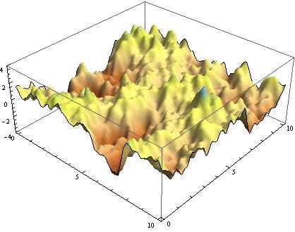
(a) Gaussian random field with Whittle-Matérn–type covariance function (see Sect. 2.2, Example 6), $a=2$, $b=\nu=1$

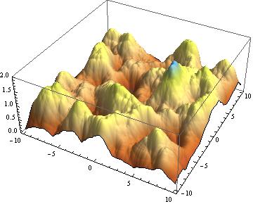
(b) Poisson shot noise field with $\lambda=1$ and $f(x)=\frac{1}{2\pi}\left(1-\frac{1}{4}\|x\|^{2}\right)\mathbf{1}(\|x\|\leq 2)$

Fig. 1: Simulated realizations of (strictly and wide sense) motion invariant random fields.

3. Boolean Random Function

Let $\{Z_{t}(x),\ x\in\mathbb{R}^{d}\}_{t\in\mathbb{R}}$ be a family of independent lower semi-continuous random functions with subgraphs having almost surely compact sections and $\Pi=\{(x_{i},t_{i})\}_{i=1}^{\infty}$ be a Poisson point process in $\mathbb{R}^{d}\times\mathbb{R}$ with intensity measure $\nu_{d}\otimes\theta$, where $\nu_{d}$ denotes the Lebesgue measure on $\mathbb{R}^{d}$ and $\theta$ is a $\sigma$-finite measure on $\mathbb{R}$. The random function

$$Z(x)=\sup\limits_{(x_{k},t_{k})\in\Pi}Z_{t_{k}}(x-x_{k}),\ \ \ x\in\mathbb{R}^{d}$$

is called a Boolean random function. The functions $Z_{t}$ are referred to as primary functions. Boolean random functions have been introduced by D. Jeulin for modelling rough morphologies (JeulinAndJeulin ), see for example (CD99, , Sect. 7.8.1) and references therein.

2.2 Elements of Correlation Theory for Square Integrable Random Fields

Let us recall the following basic concepts.

Definition 3

A symmetric function $f:\mathbb{R}^{d}\times\mathbb{R}^{d}\to\mathbb{R}$ is called positive semi–definite if for any $n\in\mathbb{N}$, $w_{1},\ldots,w_{n}\in\mathbb{C}$ and any $t_{1},\ldots,t_{n}\in\mathbb{R}^{d}$ it holds

$$\sum_{i,j=1}^{n}w_{i}\bar{w}_{j}f(t_{i},t_{j})\geq 0.$$

Definition 4

A symmetric function $f:\mathbb{R}^{d}\times\mathbb{R}^{d}\to\mathbb{R}$ is called positive definite if for any $n\in\mathbb{N}$, $w_{1},\ldots,w_{n}\in\mathbb{C}$ such that $(w_{1},\ldots,w_{n})^{\top}\neq o\in\mathbb{C}^{n}$ and any $t_{1},\ldots,t_{n}\in\mathbb{R}^{d}$ it holds

$$\sum_{i,j=1}^{n}w_{i}\bar{w}_{j}f(t_{i},t_{j})>0.$$

Definition 5

A symmetric function $f:\mathbb{R}^{d}\times\mathbb{R}^{d}\to\mathbb{R}$ is called conditionally negative semi–definite if for any $n\in\mathbb{N}$, $w_{1},\ldots,w_{n}\in\mathbb{C}$ such that $\sum_{i=1}^{n}w_{i}=0$ and any $t_{1},\ldots,t_{n}\in\mathbb{R}^{d}$ it holds

$$\sum_{i,j=1}^{n}w_{i}\bar{w}_{j}f(t_{i},t_{j})\leq 0.$$

Exercise 4

Prove that functions $\cos(a\cdot x),\ a\in\mathbb{R}$, $e^{-|x|^{p}},\ p\in(0,\ 2]$ are positive semi–definite, whereas $e^{-|x|^{p}},\ p>2$, $|\cos x|$, $a^{2}+\cos^{2}x,\ a\in\mathbb{R}$ are not.

Exercise 5

Find a positive semi-definite function with discrete support.

Covariance function

Definition 6

For a real-valued random field $X=\{X(t),\ t\in\mathbb{R}^{d}\}$ with $\mathbf{E}X(t)^{2}<\infty$, $t\in\mathbb{R}^{d}$, the function $C:\mathbb{R}^{d}\times\mathbb{R}^{d}\to\mathbb{R}$ given by

$$C(s,t)=\mathbf{c}\mathbf{o}\mathbf{v}(X(s),X(t))=\mathbf{E}\left(X(s)-\mathbb{E}X(s)\right)\left(X(t)-\mathbb{E}X(t)\right),\quad s,t\in\mathbb{R}^{d}$$

is called the covariance function.

If $X$ is wide sense stationary (motion invariant), then $C(s,t)$ depends only on $s-t$ ($\|s-t\|$, respectively), $s,t\in\mathbb{R}^{d}$. For the properties of the covariance function see (BS12, , Sect. 9.4-9.6). We mention just a few:

1. Generic property. A function $f:\mathbb{R}^{d}\times\mathbb{R}^{d}\to\mathbb{R}$ is a covariance function of some square integrable random field iff it is positive semi–definite.

   Exercise 6

   Prove this fact. Hint: Calculate the variance of linear combinations $\sum_{i=1}^{n}x_{i}X(t_{i})$ for arbitrary $n\in\mathbb{N}$, $t_{i}\in\mathbb{R}^{d}$, $x_{i}\in\mathbb{R}$.

2. Spectral representation. By Bochner-Kchinchin theorem (see, e.g., Bochner or (BS12, , Theorem 9.6)), any continuous at the origin positive semi–definite function $f:\mathbb{R}^{d}\to\mathbb{R}$ is a Fourier transform of some symmetric finite measure $\mu_{f}$ on $\mathbb{R}^{d}$. Thus for a wide sense stationary mean square continuous field $X$ with covariance function $C$ we have

   $$\mathbf{c}\mathbf{o}\mathbf{v}(X(s),X(t))=C(s-t)=\int_{\mathbb{R}^{d}}e^{i\langle x,s-t\rangle}\,\mu_{C}(dx).$$

   Here $\langle\cdot,\cdot\rangle$ is the Euclidean scalar product in $\mathbb{R}^{d}$. Measure $\mu_{C}$ is called a spectral measure of $X$. If $\mu_{C}$ is absolutely continuous with respect to the Lebesgue measure, then its density is called a spectral density. The above field $X$ has itself the spectral representation

   $$X(t)=\int_{\mathbb{R}^{d}}e^{i\langle x,t\rangle}\,\Lambda(dx),$$ (1)

   where $\Lambda(\cdot)$ is a complex-valued orthogonal random measure with $\mathbf{E}\,\Lambda(A)=0$ and $\mathbf{E}\left(\Lambda(A)\overline{\Lambda(B)}\right)=\mu_{C}(A\cap B)$ for any Borel sets $A,B\subset\mathbb{R}^{d}$. The integral in (1) is understood in the mean square sense, i.e. its integral sums converge in $L^{2}(\Omega,{\cal{F}},\mathbf{P})$. For more details on the spectral representation of stationary processes see (Bulinski2, , Sect. 7, §9, §10), (Lif12, , Sect. 3.2, pp. 20-21) or (CD99, , Sect. 2.3.3), (Wentzell, , Sect. 4.2, p. 90). The spectral representation is used e.g. to simulate stationary Gaussian random fields approximating the integral in (1) by its finite integral sums with respect to a Gaussian white noise measure $\Lambda$.

Parametric Families of Covariance Functions

1. White Noise Model

$$C(s,t)=\begin{cases}\sigma^{2},\ s=t\\ 0,\ s\neq t.\end{cases},\quad s,t\in\mathbb{R}^{d}.$$

It is a covariance function of a random field $X$ consisting of independent random variables $X(t)$, $t\in\mathbb{R}^{d}$, $d\geq 1$ with variance $\sigma^{2}>0$.

2. Normal Scale Mixture

$$C(s,t)=\int_{0}^{\infty}e^{-x\|s-t\|^{2}}\,\mu(dx),\quad s,t\in\mathbb{R}^{d}$$

for some finite measure $\mu$ on $[0,\infty)$ is the covariance function of a motion invariant random field for any $d\geq 1$ (see Schoenberg ).

3. Bessel Family

$$C(s,t)=b(a\|s-t\|)^{-\nu}J_{\nu}(a\|s-t\|),\quad\nu=\frac{d-2}{2},\quad a,b>0,\quad s,t\in\mathbb{R}^{d},$$

where

$$J_{\nu}(r)=\sum_{j=0}^{\infty}\frac{(-1)^{j}}{j!\Gamma(\nu+j+1)}\left(\frac{r}{2}\right)^{\nu+2j},\ \ r\in\mathbb{R}$$

is the Bessel function of the 1st kind of order $\nu$ (cf. Magnus ) and $d\geq 1$. The positive semi–definiteness of $C$ is proven in (Yaglom1, , p. 367). The spectral density of $C$ is given by

$$f(h)=\frac{b(a^{2}-h^{2})^{\nu-\frac{d}{2}}}{2^{\nu}\pi^{\frac{d}{2}}a^{2\nu}\Gamma(\nu+1-\frac{d}{2})}I(h\in[0,a]).$$

A special case of $d=3$, i.e., $\nu=\frac{1}{2}$ yields the so-called hole effect model

$$C(s,t)=b\frac{\sin(a\|s-t\|)}{a\|s-t\|},\quad s,t\in\mathbb{R}^{d}.$$

This model is valid only for $d\leq 3$.

4. Cauchy Family

$$C(s,t)=\frac{b}{(1+(a\|s-t\|)^{2})^{\nu}},\quad a,b,\nu>0,\quad s,t\in\mathbb{R}^{d}.$$

Up to scaling, this function is positive semi-definite as a normal scale mixture with $\mu(dx)=cx^{\nu-1}e^{-x}dx$ for some constant $c>0$.

5. Stable Family

$$C(s,t)=be^{-a\|s-t\|^{\nu}},\quad\nu\in(0,2],\quad s,t\in\mathbb{R}^{d}.$$

This function is positive semi-definite for all $d\geq 1$ since it is made by substitution $\theta\mapsto\|s-t\|$ out of the characteristic function of a symmetric $\nu$-stable random variable, cf. Definition 11. A special case ($\nu=2$) of the stable family is a Gaussian model: $C(s,t)=be^{-a\|s-t\|^{2}}$. Its spectral density is equal to $f(h)=\frac{b\sqrt{a}}{2}he^{-\frac{ah^{2}}{4}}$.

6. Whittle-Matérn Family

$$C(s,t)=W_{\nu}(\|s-t\|)=b2^{1-\nu}(a\|s-t\|)^{\nu}K_{\nu}(a\|s-t\|),\quad s,t\in\mathbb{R}^{d},\;s\neq t,$$

where $\nu,a,b>0$, $d\geq 1$ and $K_{\nu}$ is the modified Bessel function of third kind, also called Macdonald function:

$$K_{\nu}(r)=\frac{\pi}{2\sin(\pi\nu)}(e^{i\frac{\pi}{2}\nu}J_{-\nu}(re^{i\frac{\pi}{2}})-e^{-i\frac{\pi}{2}\nu}J_{\nu}(re^{-i\frac{\pi}{2}})),\quad r\in\mathbb{R},\quad\nu\not\in\mathbb{N}.$$

For $\nu=n\in\mathbb{N}$ the above definiton of $K_{\nu}$ is understood in the sense of a limit as $\nu\rightarrow n$, see (Magnus, , p. 69). For $s=t$, we set $C(t,t)=b.$ The spectral density of $C$ is given by

$$f(h)=b\frac{2\Gamma(\nu+\frac{d}{2})}{\Gamma(\frac{d}{2})\Gamma(\nu)}\frac{(ah)^{d-1}}{(1+(ah)^{2})^{\nu+\frac{d}{2}}}I(h>0).$$

If $\nu=\frac{2d+1}{2}$ then a random field with covariance function $C$ is $d$ times differentiable in mean-square sense. If $\nu=\frac{1}{2}$ then the exponential model

$$C(s,t)=be^{-a\|s-t\|},\quad s,t\in\mathbb{R}^{d}$$

is an important special case. The same exponential covariance belongs to the stable family for $\nu=1$.

Figure 1(a) shows a realization of a centered Gaussian random field $X$ with Whittle-Matérn type covariance function.

7. Spherical Model

is given for $1\leq d\leq 3$ by

$$C(s,t)=b\left(1-\frac{3}{2}\frac{\|s-t\|}{a}+\frac{1}{2}\frac{\|s-t\|^{3}}{a^{3}}\right)I(\|s-t\|\leq a),\quad a,b>0,\quad s,t\in\mathbb{R}^{d}.$$

If $d=3$ the above formula yields the volume of $B_{\frac{a}{2}}(0)\cap B_{\frac{a}{2}}(x_{0})$, where $x_{o}\in\mathbb{R}^{3}$, $\|x_{0}\|=\|s-t\|$. This is exactly the way how it can be generalized to higher dimensions:

$$C(s,t)=\nu_{d}\left(B_{\frac{a}{2}}(0)\cap B_{\frac{a}{2}}(s-t)\right),\quad s,t\in\mathbb{R}^{d},$$

where $\nu_{d}$ is the Lebesgue measure. The advantage of spherical models is that they have a compact support.

8. Geometric Anisotropy

It is easy to see that all covariance models considered above are motion invariant. An example of a anisotropic covariance structure can be provided by rotating and stretching the argument of a motion invariant covariance model. Let $C_{0}(\|h\|)$, $h\in\mathbb{R}^{d}$ be a covariance function of a motion invariant field where $C_{0}:\mathbb{R}^{+}\to\mathbb{R}^{+}$. For a positive definite $(d\times d)$–matrix $Q$,

$$C(h)=C_{0}(\sqrt{h^{T}Qh}),\quad h\in\mathbb{R}^{d}$$

is a covariance function of some wide sense stationary anisotropic random field (see (Wack03, , Chap. 9)).

9. Cyclone Model

For $d=3$, let

$$C(x,y)=\frac{2^{3/2}det(S_{x})^{1/4}det(S_{y})^{1/4}}{\sqrt{det(S_{x}+S_{y})}}W_{\nu}\left(\sqrt{(x-y)^{T}S_{x}(S_{x}+S_{y})^{-1}S_{y}(x-y)}\right),$$

where $x,y\in\mathbb{R}^{3}$, $S_{x}=Id+xx^{T}$, $Id$ is a $(3\times 3)$–identity matrix and $W_{\nu}$ is the Whittel-Matérn model. In (Sch10, , Theorem 5, Example 16), it is shown that $C$ is a valid covariance function belonging to a more general class of covariances that mimic cyclones.

Exercise 7

Show $C$ is a covariance function of isotropic but not wide sense stationary random field, i.e., $C(x,y)=C(Rx,Ry)$ for any $R\in SO_{3}$, but $C(x,y)$ does not depend on $x-y$, $x,y\in\mathbb{R}^{3}$.

For more sophisticated covariance models including spatio–temporal effects see e.g. Sch10 and references therein.

Variogram

Definition 7

For a random field $X=\{X(t),t\in\mathbb{R}^{d}\}$ the following expression

$$\gamma(t,s):=\frac{1}{2}\mathbf{E}(X(t)-X(s))^{2},\quad s,t\in\mathbb{R}^{d}$$

is called a variogram of $X$ whenever it is finite for any $s,t\in\mathbb{R}^{d}$.

For square integrable random fields $X$, it obviously holds

$$\gamma(s,t)=\frac{1}{2}\mathbf{v}\mathbf{a}\mathbf{r}X(s)+\frac{1}{2}\mathbf{v}\mathbf{a}\mathbf{r}X(t)-\mathbf{c}\mathbf{o}\mathbf{v}(X(t),X(s))+\frac{1}{2}(\mathbf{E}X(s)-\mathbf{E}X(t))^{2}.$$ (2)

If the field $X$ is intrinsic stationary of order two (motion invariant) then $\gamma(s,t)$ depends only on the difference $s-t$ ($\|s-t\|$, respectively). With slight abuse of notation in these cases, we write $\gamma(s-t)$ and $\gamma(\|s-t\|)$ for functions $\gamma:\mathbb{R}^{d}\to\mathbb{R}$ and $\gamma:\mathbb{R}_{+}\to\mathbb{R}$, respectively. For a wide sense stationary random field $X$ with covariance function $C$ the relation (2) reads

$$\gamma(h)=C(0)-C(h),\quad h\in\mathbb{R}^{d}.$$ (3)

Basic Properties of Variograms

Let $X$ be a random field with covariance function $C$ and variogram $\gamma$. The following properties hold:

1. $\gamma(t,t)=0$, $t\in\mathbb{R}^{d}$.

2. Symmetry: $\gamma(t,s)=\gamma(s,t)$, $s,t\in\mathbb{R}^{d}$.

3. Characterization of variograms:

   1. A function $\gamma:\mathbb{R}^{d}\times\mathbb{R}^{d}\to\mathbb{R}_{+}$ is a variogram of some random field if $\gamma$ is conditionally negative semi–definite, see, for example, (GSS01, , Theorem 1) or (CD99, , Sect. 2.3.3, p.61).

      Exercise 8

      Prove that the variogram of any intrinsic stationary random field $X$ is a conditionally negative semi–definite function.
      Hint: Calculate $Var(\sum_{i=1}^{n}\lambda_{i}X(t_{i}))$ applying (2) with $\sum_{i=1}^{n}\lambda_{i}=0$.

   2. A continuous even function $\gamma:\mathbb{R}^{d}\rightarrow\mathbb{R}_{+}$ with $\gamma(0)=0$ is a variogram of a wide sense stationary random field if $e^{-\lambda\gamma}$ is a covariance function for all $\lambda>0$, cf. Schoenberg38b .

4. Stability: If $\gamma_{1},\gamma_{2}$ are variograms then $\gamma=\gamma_{1}+\gamma_{2}$ is a variogram as well.

   Exercise 9

   Prove this fact. Show in particular that $\gamma(h)=\gamma_{1}(h_{i})+\gamma_{2}(h_{j}),$ where $h=(h_{1},\ldots,h_{d})^{\top}\in\mathbb{R}^{d}$ and $\gamma_{1},$ $\gamma_{2}$ are univariate variograms, is a variogram.

5. Mixture: Let $\gamma_{x}:\mathbb{R}^{d}\to\mathbb{R}_{+}$ be a variogram of an intrinsic stationary (of order two) random field for any $x\in\mathbb{R}$. Then the function

   $$\gamma(t)=\int_{\mathbb{R}}\gamma_{x}(t)\mu(dx),\quad t\in\mathbb{R}^{d}$$

   is a variogram of some random field if $\mu$ is a measure on $\mathbb{R}$ and the above integral exists for any $t\in\mathbb{R}^{d}$, see (CD99, , Sect. 2.3.2, pp. 60-61).

6. If $X$ is wide sense stationary and $C(\infty):=\lim_{\|h\|\rightarrow\infty}C(h)=0$, then it follows from (3) that there exists the so-called sill $\gamma(\infty):=\lim_{\|h\|\rightarrow\infty}\gamma(h)=C(0)$.

7. If $X$ is mean square continuous then $\gamma(h)\leq c\|h\|^{2}$, $h\in\mathbb{R}^{d}$ for a constant $c>0$ and large $\|h\|$, see (Yaglom1, , pp. 397-398).

8. If $X$ is mean square differentiable then $\lim_{\|h\|\rightarrow\infty}\frac{\gamma(h)}{\|h\|^{2}}=0$, see (Yaglom2, , pp. 136-137).

9. Let $\gamma:\mathbb{R}\to\mathbb{R}_{+}$ be an even twice continuously differentiable function with $\gamma(0)=0$. Then $\gamma$ is a variogram iff $\gamma^{\prime\prime}$ is a covariation function, cf. (GSS01, , Theorem 7).

Exercise 10

Show that for a variogram $\gamma$ the function $e^{\lambda\gamma}$ is a variogram for any $\lambda>0$.

Exercise 11

Let a bounded function $\gamma:\mathbb{R}^{d}\to\mathbb{R}_{+}$ be the variogram of some intrinsic stationary of order two real valued random field $X$. Consider $C(x,y)=\gamma(x)+\gamma(y)-\gamma(x-y)$, $x,y\in\mathbb{R}^{d}$. Show that $C$ is a covariance function of a random field $Z$ such that $Z(0)=0$ a.s.

Parametric families of variograms

Most parametric models for variograms of stationary random fields, which are widely used in applications, can be constructed from the corresponding families of covariance functions (such as those described in Sect. 2.2) by applying the relation (3) as well as stability and geometric anisotropy properties. Most models of variograms inherit their names from the corresponding covariance models (e.g., exponential, spherical one). One of few exceptions is the variogram corresponding to the white noise which is called nugget effect.

Stability property can be also used to create different anisotropy effects, for instance, the so-called purely zonal anisotropy. To explain this on an example, let $\gamma(h)=a\gamma_{1}(h_{x})+b\gamma_{2}(h_{y})+c\gamma_{3}(h_{z})$, $h=(h_{x},h_{y},h_{z})\in\mathbb{R}^{3}$, $a,b,c\geq 0$, where $\gamma_{i}$ $i=1,2,3$ are variograms in dimension $d=1$. Then $\gamma$ is a variogram in dimension $d=3$ which allows for different dependence ranges in three different axes directions. An example of mixed anisotropy models is

$$\gamma(h)=\gamma_{1}(\|h\|)+\gamma_{2}\left(\sqrt{h_{x}^{2}+h_{y}^{2}}\right)+\gamma_{3}(h_{z}),\ h=(h_{x},h_{y},h_{z})\in\mathbb{R}^{3}.$$

This is a mixture of 3D-isotropic variogram $\gamma_{1}$, 2D-isotropic (in the xy-plane) variogram $\gamma_{2}$ and a 1D-variogram $\gamma_{3}$. Addition of a linear combination of $\gamma_{2}$ and $\gamma_{3}$ creates anisotropy in direction of z-axis.

See more about variograms in (CD99, , Chap. 2).

Statistical Estimation of Covariances and Variograms

The numerous approaches to estimate a covariance function or a variogram are well described in the literature and therefore will not be reviewed here. An interested reader can see e.g. (CD99, , Sect. 2.2) and (BS12, , Sect. 9.8) and references therein.

Example 1

To illustrate the above theory, consider microscopic steel data (figure 2(a)). This data is obviously isotropic. Figure 2(b) shows estimates for the corresponding variogram. For this purpose Mathéron’s estimator (see (BS12, , p. 325)) was calculated for different directions and $0\leq h\leq 0.5$. The directions can be distinguished by the color of their plots. Since these data are isotropic the estimates differ not too much.

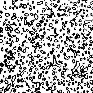
(a) Microscopic image of a steel surface.

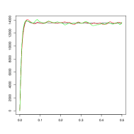
(b) Estimates for the x-direction (red), y-direction (green), all directions (black) for values $0\leq h\leq 0.5$.

Fig. 2: Microscopic steel image (left) and its empirical variogram estimated in different directions (right)

Example 2

Let us construct an example of zonally anisotropic variogram, in which the value for the sill depends on the direction of the input vector $h$. Consider

$$\gamma(h)=\gamma_{1}(h)+\gamma_{2}(h)$$

where $\gamma_{1}$ is an isotropic variogram

$$\gamma_{1}(h)=1-e^{-|h|},\ \ \ h\in\mathbb{R}^{2}$$

and $\gamma_{2}$ is a geometrical anisotropic variogram model

$$\gamma_{2}(h)=1-e^{-\frac{\sqrt{h^{T}Qh}}{5}},\ \ \ h\in\mathbb{R}^{2}$$

with $Q=\sqrt{\Lambda}\cdot R$ with $R$ being a rotation matrix with rotation angle $\alpha=2$ and $\Lambda=diag(5,1)$ being a diagonal matrix. Figure 3(a) shows $\gamma$ on $[-1,1]^{2}$. Figure 3(b) illustrates the elliptic form of the contour lines of a zonally anisotropic variogram.

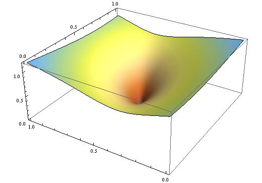
(a) Zonally anisotropic model with rotation angle $\alpha=2$ and scaling factors $\lambda_{1}=5$, $\lambda_{2}=1$.

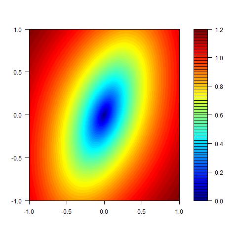
(b) Contour lines of 3(a)

Fig. 3: Zonally anisotropic theoretical variogram

2.3 Stable Random Fields

In this Section, we review the basic notions of the theory of stable distributions, random measures and fields. A very good reference which covers most of this topic is ST94 , see also Nol , (Sat99, , Chapter 3), Zol86 , etc.

Stable Distributions

Let $n\in\mathbb{N}$. We begin with the definition of stability for random vectors.

Stable Random Vectors

Definition 8

A random vector $\boldsymbol{X}=(X_{1},\ldots,X_{n})^{\mathsf{T}}$ in $\mathbb{R}^{n}$ is called stable if for all $m\geq 2$ there exist $c=c(m)>0$ and $k=k(m)\in\mathbb{R}^{n}$ such that

$$\boldsymbol{X}^{(1)}+\boldsymbol{X}^{(2)}+...+\boldsymbol{X}^{(m)}\buildrel d\over{=}c\boldsymbol{X}+k,$$

where $\{\boldsymbol{X}^{(i)}\}_{i=1}^{m}$ are independent copies of $\boldsymbol{X}$.

It can be shown that $c=m^{1/\alpha}$ for some $0<\alpha\leq 2$ which is called the stability index, see (ST94, , Theorem 2.1.2). There is an equivalent definition of stable vectors which is often used in mathematical practice to check stability.

Definition 9

Let $\alpha\in(0,2)$. We say that a random vector $\boldsymbol{X}=(X_{1},\ldots,X_{n})^{\mathsf{T}}$ in $\mathbb{R}^{n}$ is $\alpha$-stable if its characteristic function is given by

$$\varphi_{\boldsymbol{X}}(\boldsymbol{\theta})=\begin{cases}e^{-\int_{\mathbb{S}^{n-1}}|\langle\boldsymbol{\theta},\boldsymbol{s}\rangle|^{\alpha}\left(1-i\text{sign}(\langle\boldsymbol{\theta},\boldsymbol{s}\rangle)\tan\frac{\pi\alpha}{2}\right)\Gamma(d\boldsymbol{s})+i\langle\boldsymbol{\theta},\boldsymbol{\mu}\rangle},&\alpha\neq 1,\\ e^{-\int_{\mathbb{S}^{n-1}}|\langle\boldsymbol{\theta},\boldsymbol{s}\rangle|\left(1+i\frac{2}{\pi}\text{sign}(\langle\boldsymbol{\theta},\boldsymbol{s}\rangle)\ln|\langle\boldsymbol{\theta},\boldsymbol{s}\rangle|\right)\Gamma(d\boldsymbol{s})+i\langle\boldsymbol{\theta},\boldsymbol{\mu}\rangle},&\alpha=1,\end{cases}$$ (4)

where $\Gamma$ is a finite measure on the unit sphere $\mathbb{S}^{n-1}$ of $\mathbb{R}^{n}$ and $\boldsymbol{\mu}$ is an arbitrary vector in $\mathbb{R}^{n}$.

The pair $(\boldsymbol{\mu},\Gamma)$ gives a unique parametrization of the distribution of $\alpha$-stable random vectors for $\alpha\in(0,2)$, and we write $X\sim S_{\alpha}(\boldsymbol{\mu},\Gamma).$ This means that there is no other pair $(\mu^{\prime},\Gamma^{\prime})$ yielding the same characteristic function $\varphi_{X}$ in (4). The measure $\Gamma$ is called spectral measure of $X$ and contains all the information about the dependence between the vector components $X_{i}$ (see also Exercise 15). The vector $\boldsymbol{\mu}$ reflects the shift with respect to the origin.

Definition 10

A random vector $X=(X_{1},\ldots,X_{n})^{\top}$ is called singular if $\sum_{i=1}^{n}c_{i}X_{i}=0$ a.s. for some $(c_{1},\ldots,c_{n})^{\mathsf{T}}\in\mathbb{R}^{n}\setminus\{0\}$. Otherwise, it is called full-dimensional.

If $\alpha=2$, then Definition 8 yields a Gaussian random vector which is equivalently defined via its characteristic function

$$\varphi_{\boldsymbol{X}}(\mathbf{\theta})=\exp\left\{i\langle\mathbf{\theta},\boldsymbol{\mu}\rangle-\tfrac{1}{2}\mathbf{\theta}^{\mathsf{T}}\boldsymbol{\Sigma}\mathbf{\theta}\right\}.$$ (5)

Here $\mu\in\mathbb{R}^{n}$ is the mean of $X$ and $\Sigma$ is a symmetric, positive semi–definite $(n\times n)$–covariance matrix of $X$. The matrix $\Sigma$ has the elements $\sigma_{{ij}}=\mathbf{E}(X_{i}-\mu_{i})(X_{j}-\mu_{j})$, where $X_{i}$ and $\mu_{i}$ are the components of vectors $X$ and $\mu$, respectively. It is easy to see that if $\det\Sigma=0$ then the Gaussian random vector $\boldsymbol{X}$ is singular.

Exercise 12

Prove that Definition 8 is equivalent to Definition 9 for $\alpha\in(0,2)$, and it is equivalent to the definition of a Gaussian random vector via relation (5) for $\alpha=2$.

Exercise 13

Show that for $X\sim S_{\alpha}(\mu,\Gamma)$ the relation between the drift $k$ in Definition 8 and the shift $\mu$ in Definition 9 is $k(m)=\mu(m-m^{1/\alpha})$. Hint: First show that $\sum_{i=1}^{m}X^{(i)}\sim S(m\mu,m\Gamma)$ and $m^{1/\alpha}X+k(m)\sim S(m^{1/\alpha}\mu+k(m),m\Gamma)$.

Remark 1

For $\alpha=2$, the characteristic function (4) has the form

$$\varphi(\boldsymbol{\theta})=\exp\left\{-\int_{\mathbb{S}^{n-1}}\langle\boldsymbol{\theta},\boldsymbol{s}\rangle^{2}\Gamma(d\boldsymbol{s})+i\langle\boldsymbol{\theta},\boldsymbol{\mu}\rangle\right\}.$$ (6)

It is easy to find two different finite measures $\Gamma_{1}$ and $\Gamma_{2}$ on $\mathbb{S}^{n-1}$ yielding the same function $\varphi$ in this case.

Exercise 14

Check that the following two finite measures on the unite sphere in $\mathbb{R}^{2}$

$$\Gamma_{1}(ds)=\delta_{(\sqrt{2}/2,\sqrt{2}/2)}(ds)+\delta_{(-\sqrt{2}/2,-\sqrt{2}/2)}(ds),$$

$$\Gamma_{2}(ds)=2\delta_{(\sqrt{2}/2,\sqrt{2}/2)}(ds)$$

and a shift $\mu\in\mathbb{R}^{2}$ yield the same expression in (4) if $\alpha=2$, $n=2$. Here $\delta_{x}(\cdot)$ is the Dirac measure concentrated at the point $x\in\mathbb{R}^{2}$. Verify that this expression corresponds to the characteristic function of the Gaussian vector with shift $\mu$ and covariance matrix

$$\Sigma=\begin{pmatrix}2&2\\ 2&2\end{pmatrix}.$$

A random vector $\boldsymbol{X}$ in $\mathbb{R}^{n}$ is called symmetric if $\mathbb{P}(\boldsymbol{X}\in A)=\mathbb{P}(-\boldsymbol{X}\in A)$ for any Borel set $A\in\mathbb{R}^{n}$. For symmetric $\alpha$-stable distributions, we use the standard abbreviation $S\alpha S$.

Lemma 1 (ST94 , Theorem 2.4.3)

An $\alpha$–stable random vector $X$ is symmetric iff its shift $\mu=0$ and spectral measure $\Gamma$ is symmetric.

Exercise 15

Let $X=(X_{1},X_{2})^{T}$ be an $\alpha$-stable random vector, $\alpha\in(0,2)$, with the spectral measure $\Gamma$. Let $supp{(\Gamma)}$ be the support of $\Gamma$. Show that

• $X_{1}$ is independent of $X_{2}$ iff $supp{(\Gamma)}$ lies within the intersection of the sphere with the coordinate axes.

• $X_{1}=c\cdot X_{2}$ a.s. for some $c\in\mathbb{R}$ (i.e. the vector $X$ is singular) iff $supp{(\Gamma)}$ is a subset of the unite sphere intersected by a hyperplane.

Stable Random Variables

If $n=1$ we deal with stable random variables whose distribution laws are defined by four parameters $\alpha$, $\sigma$, $\beta$, and $\mu$.

Definition 11

The random variable $X$ is called $\alpha$-stable if its characteristic function has the form

$$\varphi_{X}(\theta)=\begin{cases}\exp\left\{-\sigma^{\alpha}|\theta|^{\alpha}\left(1-i\beta(\text{sign}(\theta))\tan\frac{\pi\alpha}{2}\right)+i\mu\theta\right\},&\alpha\in(0,2],\alpha\neq 1,\\ \exp\left\{-\sigma|\theta|\left(1+i\beta\frac{2}{\pi}(\text{sign}(\theta))\ln|\theta|\right)+i\mu\theta\right\},&\alpha=1.\end{cases}$$

We write $X\sim S_{\alpha}(\sigma,\beta,\mu)$.

Compared with representation (4), two new parameters $\sigma\geq 0$ and $\beta\in[-1,1]$ introduced in lieu of the spectral measure $\Gamma$ are interpreted as parameters of scale and skewness, respectively.

Exercise 16

Show that the spectral measure of $X\sim S_{\alpha}(\sigma,\beta,\mu)$ is given by

$$\Gamma(ds)=\frac{\sigma^{\alpha}}{2}(1+\beta)\delta_{1}(ds)+\frac{\sigma^{\alpha}}{2}(1-\beta)\delta_{-1}(ds).$$

Hence, it holds

$$\sigma^{\alpha}=\Gamma(\{1\})+\Gamma(\{-1\}),\qquad\beta=\frac{\Gamma(\{1\})-\Gamma(\{-1\})}{\Gamma(\{1\})+\Gamma(\{-1\})}.$$

Remark 2

Stable distributions are absolutely continuous. Nevertheless, their densities are not known in the closed form except for the cases $\alpha=1/2$, $\alpha=1$ and $\alpha=2$.

Example 3

1. $X\sim S_{2}(\sigma,0,\mu)$ is a Gaussian random variable with mean $\mu$ and variance $2\sigma^{2}$.

2. Random variable $X\sim S_{\alpha}(\sigma,\pm 1,\mu)$ is called totally skewed. Notice that if $\alpha\in[1,2)$ then $X$ attains values in the whole $\mathbb{R}$. On the contrary, if $\alpha\in(0,1)$ and $\mu=0$, then $X\geq 0$, $(X\leq 0)$ a.s. when $\beta=1$ $(\beta=-1)$, respectively.

Exercise 17

Show that the characteristic function of $S\alpha S$ random variable $X$ is equal to $\varphi_{X}({\theta})=\exp\{-\sigma^{\alpha}|\theta|^{\alpha}\}$, i.e., $X\sim S_{\alpha}(\sigma,0,0)$ for some $\sigma>0$.

Tails and Moments

The non–Gaussian stable distributions are fat tailed. This means that they belong to a subclass of heavy tailed distributions with especially slow large deviation behavior, see more details on heavy tailed distributions e.g. in FKZ11 , Mar07 , etc. Namely, for $X\sim S_{\alpha}(\sigma,\beta,\mu)$ with $\alpha\in(0,2)$ there exists $c>0$ such that

$$\mathbf{P}(|X|>x)\sim cx^{-\alpha},\ x\to\infty.$$ (7)

Here and in what follows we say that $a_{x}\sim b_{x}$ if $\lim_{x\to\infty}\frac{a_{x}}{b_{x}}=1$. As a corollary of (7), the absolute moments of $X$ behave like

$$\mathbf{E}|X|^{p}=\int_{0}^{\infty}\mathbf{P}\{|X|>x^{1/p}\}dx\approx c_{1}\int_{0}^{\infty}x^{-\alpha/p}dx.$$

They are finite if $p\in(0,\alpha)$ and infinite for any $p\in[\alpha,\infty)$.

Exercise 18

Show that

• normal distribution $X\sim N(\mu,\sigma^{2})$ is not heavy tailed (this is equivalent to the statement that the tails are exponentially bounded), i.e.,

  $$\mathbf{P}(X<-x)=\mathbf{P}(X>x)\sim\frac{1}{\sqrt{2\pi}\sigma x}e^{-x^{2}/(2\sigma^{2})},\quad x\to\infty.$$

• for $X\sim S_{\alpha}(\sigma,\beta,0)$, $\alpha\in(0,2)$, $\alpha\neq 1$ it holds

  $$\left(\mathbf{E}|X|^{p}\right)^{1/p}=c_{\alpha,\beta}(p)\sigma$$ (8)

  for every $p\in(0,\alpha)$. Here $c_{\alpha,\beta}(p)=(\mathbf{E}|\xi|^{p})^{1/p}$ with $\xi\sim S_{\alpha}(1,\beta,0)$. If $\alpha=1$ then equation (8) holds only for $\beta=0$.

• for any $\alpha$-stable random variables $X$ and $Y$ the sum $aX+bY$, $a,b\in\mathbb{R}$ is again $\alpha$-stable. Moreover, components $X_{i}$ of the stable vector $X=(X_{1},X_{2})\sim S_{\alpha}(\mu,\Gamma)$ are stable, and it holds $\sigma_{aX_{1}+bX_{2}}=\int_{\mathbb{S}^{1}}|as_{1}+bs_{2}|^{\alpha}\Gamma(ds_{1},ds_{2})$ for any $a,b\in\mathbb{R}$.

Simulation of stable random variables is extensively described in Nol .

Integration with Respect to Stable Random Measures

Let $(E,\mathcal{E},m)$ be an arbitrary measurable space with $\sigma$-finite measure $m$ and $\mathcal{E}_{0}:=\{A\in\mathcal{E}:m(A)<\infty\}$. Let $\beta:E\to[-1,1]$ be a measurable function.

Definition 12

A random function $M=\{M(A),\;A\in\mathcal{E}_{0}\}$ is called an independently scattered random measure (random noise) if

1. for any $n\in\mathbb{N}$ and pairwise disjoint sets $A_{1},A_{2},\ldots,A_{n}\in\mathcal{E}_{0}$ random variables $M(A_{1}),\ldots,M(A_{n})$ are independent,

2. $M(\bigcup_{j=1}^{\infty}A_{j})=\sum_{j=1}^{\infty}M(A_{j})$ a.s. for a sequence of disjoint sets $A_{1},A_{2},\ldots\in\mathcal{E}_{0}$ with $\bigcup_{j=1}^{\infty}A_{j}\in\mathcal{E}_{0}$.

Definition 13

An independently scattered random measure $M$ on $(E,\mathcal{E}_{0})$ is called $\alpha$-stable if for each $A\in\mathcal{E}_{0}$

$$M(A)\sim S_{\alpha}\left((m(A))^{1/\alpha},\frac{\int_{A}\beta(x)m(dx)}{m(A)},0\right).$$

Measure $m$ is called control measure, and $\beta$ is the skewness function of $M$.

Our goal is to define an integral $\int_{E}f(x)M(dx)$ of a deterministic function $f:E\to\mathbb{R}$ with respect to an $\alpha$-stable random measure $M$. For a simple function $f(x)=\sum_{i=1}^{n}c_{i}1_{A_{i}}(x)$, where $\{A_{i}\}_{i=1}^{n}\subset\mathcal{E}_{0}$ are pairwise disjoint, we set

$$\int_{E}f(x)M(dx)=\sum_{i=1}^{n}c_{i}M(A_{i}).$$

It can be shown that, so defined, the integral $\int_{E}f(x)M(dx)$ does not depend on the representation of $f$ as a simple function, see (ST94, , Sect.3.4). For an arbitrary $f:E\to\mathbb{R}$ such that $\int_{E}|f(x)|^{\alpha}m(dx)<\infty$ consider a pointwise approximation of $f$ by simple functions $f^{(n)}$. Then we set

$$\int_{E}f(x)M(dx)=\mbox{plim}_{n\to\infty}\int_{E}f^{(n)}(x)M(dx).$$

Here plim denotes the limit in probability. This definition is independent of the choice of the approximating sequence $\{f^{(n)}\}$, cf. (ST94, , Sect. 3.4) for more details.

Lemma 2

Let $X=\int_{E}f(x)M(dx)$, where $M$ is an $\alpha$-stable random measure with control measure $m$ and skewness function $\beta$. Then $X$ is an $\alpha$-stable random variable with zero shift, scale parameter

$$\sigma_{X}^{\alpha}=\int_{E}|f(x)|^{\alpha}m(dx),$$ (9)

and skewness parameter

$$\beta_{X}=\frac{\int_{E}f(x)^{<\alpha>}\beta(x)\,m(dx)}{\int_{E}|f(x)|^{\alpha}\,m(dx)},$$

where $a^{<p>}=sign(a)\cdot|a|^{p}.$

For the proof see (ST94, , Sect.3.4). Notice that if $\beta(x)=0$ for all $x\in E$ then the integral $X$ is a $S\alpha S$ random variable.

In case of stable vectors with an integral representation, we have the following criterion of their full–dimensionality / singularity.

Lemma 3

Consider a $n$–dimensional $\alpha$–stable random vector $\vec{X}=(X_{1},\ldots,X_{n})^{\mathsf{T}}$ with $0<\alpha\leq 2$ and integral representation

$$\vec{X}=\left(\int_{E}f_{1}(x)M(dx),\ldots,\int_{E}f_{n}(x)M(dx)\right)^{\mathsf{T}}.$$

Then $\vec{X}$ is singular if and only if $\sum_{i=1}^{n}c_{i}f_{i}(x)=0$ $m$–almost everywhere for some vector $(c_{1},\ldots,c_{n})^{\mathsf{T}}\in\mathbb{R}^{n}\setminus\{0\}$.

The proof of Lemma 3 follows from Definition 10 and the fact that $\sigma_{\sum_{i=1}^{n}c_{i}X_{i}}^{\alpha}=\int_{E}\left|\sum_{i=1}^{n}c_{i}f_{i}(x)\right|^{\alpha}m(dx)$, see relation (9).

Remark 3

A more universal criterion of singularity for stable random vectors is in terms of their spectral measure. If measure $\Gamma(ds)$ on $\mathbb{S}^{n-1}$ is a spectral measure of an $\alpha$-stable vector $\vec{X}$ in $\mathbb{R}^{n}$ and is concentrated on the intersection of $\mathbb{S}^{n-1}$ with a $(n-1)$–dimensional linear subspace, then the random vector $\vec{X}$ is singular. Otherwise, $\vec{X}$ is full–dimensional. For the proof see KSS13 .

Stable Random Fields with an Integral Spectral Representation

Definition 14

A random field $X$ is called $\alpha$-stable if all its finite-dimensional distributions are $\alpha$-stable.

Consider random fields $X=\{X(t),\,t\in\mathbb{R}^{d}\}$ of the form

$$X(t)=\int_{E}f_{t}(x)\,M(dx),\quad t\in\mathbb{R}^{d},$$ (10)

where $f_{t}:E\to\mathbb{R}$ are measurable functions such that $\int_{E}|f_{t}(x)|^{\alpha}m(dx)<\infty$ and in the case $\alpha=1$ additionally $\int_{E}|f(x)\beta(x)\ln|f(x)||m(dx)<\infty$ for any $t\in\mathbb{R}^{d}$. Here $M$ is an $\alpha$-stable random measure on $(E,\mathcal{E}_{0})$ with control measure $m$ and skewness function $\beta$. Obviously, the marginals of the random field $X$ in (10) are $\alpha$-stable. If $\beta(x)=0$ for all $x\in E$ then all finite-dimensional distributions of $X$ are symmetric $\alpha$-stable, so we call $X$ to be a $S\alpha S$ random field.

A natural question is which stable fields allow for an integral representation (10). A necessary and sufficient condition for this is the condition of separability of $X$ in probability, see (ST94, , Theorem 13.2.1).

Definition 15

A stable random field $X=\{X(t),\ t\in M\}$, $M\subseteq\mathbb{R}^{d}$ is separable in probability if there exists a countable subset $M_{0}\subseteq M$ such that for every $t\in M$ and any sequence $\{t_{k}\}_{k\in\mathbb{N}}\subset M_{0}$ with $t_{k}\to t$ as $k\to\infty$ it holds $X(t)=\mbox{plim}_{k\to\infty}X(t_{k})$.

In particular, all stochastically continuous $\alpha$-stable random fields are separable in probability.

2.4 Dependence Measures for Stable Random Fields

The dependence of two $\alpha$-stable random variables cannot be digitized by using the covariance because of the absence of the second moments if $\alpha<2$. We consider two different ways of measuring the degree of dependence of two stable random variables.

Covariation

Definition 16

Let $\boldsymbol{X}=(X_{1},X_{2})^{\top}$ be an $\alpha$-stable random vector with $\alpha\in(1,2]$ and spectral measure $\Gamma$. The covariation of $X_{1}$ on $X_{2}$ is the real number

$$\left[X_{1},X_{2}\right]_{\alpha}=\int_{\mathbb{S}^{1}}s_{1}s_{2}^{<\alpha-1>}\Gamma(ds_{1},ds_{2}).$$

It has the following properties.

Theorem 2.1 (Properties of Covariation)

Let $(X_{1},X_{2},X_{3})^{\top}$ be an $\alpha$-stable random vector with $\alpha\in(1,2]$.

1. Linearity in the first entry: for $a,b\in\mathbb{R}$ it holds

   $$[aX_{1}+bX_{2},X_{3}]_{\alpha}=a[X_{1},X_{3}]_{\alpha}+b[X_{2},X_{3}]_{\alpha}.$$

2. If $X_{1}$ and $X_{2}$ are independent then $[X_{1},X_{2}]_{\alpha}=0$.

3. Gaussian case: for $\alpha=2$, it holds $\left[X_{1},X_{2}\right]_{2}=1/2\cdot\mathbf{c}\mathbf{o}\mathbf{v}(X_{1},X_{2})$.

4. Covariation and mixed moments: Let $1<\alpha<2$ and $\Gamma$ be spectral measure of $(X_{1},X_{2})^{\top}$ with $X_{1}\sim S_{\alpha}(\sigma_{1},\beta_{1},0)$, $X_{2}\sim S_{\alpha}(\sigma_{2},\beta_{2},0)$. For $1\leq p<\alpha$, it holds

   $$\frac{\mathbb{E}\left(X_{1}X_{2}^{<p-1>}\right)}{\mathbb{E}|X_{2}|^{p}}=\frac{[X_{1},X_{2}]_{\alpha}(1-c\cdot\beta_{2})+c\cdot(X_{1},X_{2})_{\alpha}}{\sigma_{2}^{\alpha}},$$ (11)

   where $(X_{1},X_{2})_{\alpha}=\int_{\mathbb{S}^{1}}s_{1}|s_{2}|^{\alpha-1}\Gamma(ds)$ and

   $$c=\frac{\tan(\alpha\pi/2)}{1+\beta_{2}^{2}\tan^{2}(\alpha\pi/2)}\left[\beta_{2}\tan(\alpha\pi/2)-\tan\left(\frac{p}{\alpha}\arctan(\beta_{2}\tan(\alpha\pi/2))\right)\right].$$

Proof

1. Linearity in the first argument is obvious. However, the covariation is not symmetric, so that there is no linearity in the second argument.

2. To see this, use Exercise 15.

3. The assertion (together with the useful relation $\mathbf{v}\mathbf{a}\mathbf{r}X_{i}=2\int_{\mathbb{S}^{1}}s_{i}^{2}\Gamma(ds_{1},ds_{2})$, $i=1,2$) follows from the comparison of the characteristic function $\varphi(\theta)$ of the Gaussian random vector $(X_{1},X_{2})^{\top}$ in representations (5) and (6).

4. See KSS12 for the proof.

Remark 4

If $X_{2}$ is symmetric, i.e. $\beta_{2}=0$, then $c=0$ and formula (11) has the following simple form

$$\frac{\mathbb{E}\left(X_{1}X_{2}^{<p-1>}\right)}{\mathbb{E}|X_{2}|^{p}}=\frac{[X_{1},X_{2}]_{\alpha}}{\sigma_{2}^{\alpha}},$$

which allows for the estimation of $[X_{1},X_{2}]_{\alpha}$ via empirical mixed moments of $X_{1}$ and $X_{2}$.

For a stable random field $X$ with integral representation (10), the covariation can be calculated by the formula

$$[X(t_{1}),X(t_{2})]_{\alpha}=\int_{E}f_{t_{1}}(x)(f_{t_{2}}(x))^{<\alpha-1>}dm(x).$$ (12)

Notice that its proof given in (ST94, , Proposition 3.5.2) for the $S\alpha S$ case holds true for skewed random fields as well.

Codifference

Drawbacks of the covariation are the lack of symmetry and the impossibility to define it for $\alpha\in(0,1]$. The following measure of dependence does not have these drawbacks. That is however compensated by a mathematically less convenient form.

Definition 17

Let $(X_{1},X_{2})^{\top}$ be an $\alpha$-stable vector. The codifference of $X_{1}$ and $X_{2}$ is

$$\tau(X_{1},X_{2})=\sigma_{X_{1}}+\sigma_{X_{2}}-\sigma_{X_{1}-X_{2}},$$

where $\sigma_{Y}$ is the scale parameter of a $\alpha$-stable random variable $Y$.

Theorem 2.2 (Properties of Codifference)

1. Symmetry: $\tau(X_{1},X_{2})=\tau(X_{2},X_{1})$.

2. If $X_{1}$ and $X_{2}$ are independent then $\tau(X_{1},X_{2})=0$. The inverse statement holds only for $\alpha\in(0,1)$.

3. Gaussian case: for $\alpha=2$, it holds $\tau(X_{1},X_{2})=\mathbf{c}\mathbf{o}\mathbf{v}(X_{1},X_{2})$.

4. Let $(X_{1},X_{2})$ and $(X^{\prime}_{1},X^{\prime}_{2})$ be S$\alpha$S vectors such that $\sigma_{X_{1}}=\sigma_{X_{2}}=\sigma_{X^{\prime}_{1}}=\sigma_{X^{\prime}_{2}}$. If $\tau(X_{1},X_{2})\leq\tau(X^{\prime}_{1},X^{\prime}_{2})$ then for any $c>0$

   $$P\{|X_{1}-X_{2}|>c\}\geq P\{|X^{\prime}_{1}-X^{\prime}_{2}|>c\},$$

   i.e., the larger the codifference, the greater the dependence.

Proof

1. Symmetry is obvious.

2. Use Exercise 18 to see the first part of the statement. Now let $\tau(X_{1},X_{2})=0$. It holds $\sigma_{X_{1}}+\sigma_{X_{2}}=\sigma_{X_{1}-X_{2}}$ iff

   $$\int_{\mathbb{S}^{1}}|s_{1}|^{\alpha}\Gamma(ds)+\int_{\mathbb{S}^{1}}|s_{2}|^{\alpha}\Gamma(ds)=\int_{\mathbb{S}^{1}}|s_{1}-s_{2}|^{\alpha}\Gamma(ds).$$

   We know however that $|s_{1}-s_{2}|^{\alpha}=|s_{1}|^{\alpha}+|s_{2}|^{\alpha}$ iff $\alpha<1$ and $s_{1}s_{2}=0$.

3. It holds $\tau(X_{1},X_{2})=1/2(\mathbf{v}\mathbf{a}\mathbf{r}\,X_{1}+\mathbf{v}\mathbf{a}\mathbf{r}\,X_{2}-\mathbf{v}\mathbf{a}\mathbf{r}(X_{1}-X_{2}))=\mathbf{c}\mathbf{o}\mathbf{v}(X_{1},X_{2})$.

4. See (ST94, , Property 2.10.6) for the proof.

2.5 Examples of Stable Processes and Fields

1. Stable Lévy Process

This is a process defined by $X(t)=M\left([0,t]\right)$, $t\in\mathbb{R}_{+}$ where $M$ is an $\alpha$-stable measure on $\mathbb{R}_{+}$ with skewness function $\beta$ and Lebesgue control measure multiplied by $\sigma>0$. $X$ has representation (10) with $f_{t}(x)=\mathbf{1}(x\in[0,t])$. It obviously holds $X(0)=0$ a.s. Moreover, $X$ has independent and stationary increments.

Depending on $\beta$ the skewness of the process may vary. So, for $\alpha<1$ and $\beta\equiv 1$ we obtain a stable Lévy process with non-decreasing sample paths, the so–called stable subordinator. To see this use one-to-one correspondence between the infinitely divisible distributions and the Lévy processes, thus $X(1)\sim S_{\alpha}(\sigma,1,0)$ corresponds to a Lévy process with the triplet $(0,0,\frac{\sigma\alpha}{\Gamma(1-\alpha)cos(\pi\alpha/2)}\frac{dx}{x^{\alpha+1}}\mathbf{1}(x>0))$, which has only positive integrable jumps, see also (Sat99, , Examples 21.7 and 24.12).

2. Stable Moving Average Random Fields

A stable moving average $X=\{X(t),\;t\in\mathbb{R}^{d}\}$ is defined by the formula

$$X(t)=\int_{\mathbb{R}^{d}}f(t-s)M(ds),\quad t\in\mathbb{R}^{d},$$

where $f\in L^{\alpha}(\mathbb{R}^{d})$ is called a kernel function and $M$ is an $\alpha$–stable random measure with Lebesgue control measure. It can be easily seen that $X$ is strictly stationary. See Figures 4(a) and 4(b) for simulated realizations of moving averages in $d=2$ with the bisquare and the cylindric kernels.

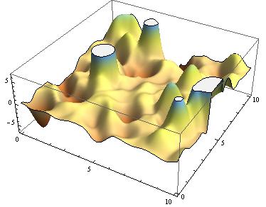
(a) ​​​ Bisquare ​ kernel ​ $f(x)=\frac{15}{16}\left(1-\|x\|^{2}\right)^{2}\mathbf{1}\left(x\in B_{1}(0)\right)$.

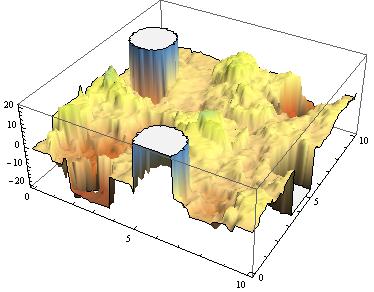
(b) Cylindric kernel $f(x)=\mathbf{1}\left(x\in B_{1}(0)\right)$, $x\in\mathbb{R}^{2}$.

Fig. 4: Continuous (left) and discontinuous (right) realization of a $0.8$-stable moving average random field with $S\alpha S$ random measure $M$.

Stable Ornstein–Uhlenbeck process is a stable moving average process $X(t)=\int_{-\infty}^{t}e^{-\lambda(t-s)}M(ds)$, $t\in\mathbb{R}$ where $M$ is a $S\alpha S$ random measure on $\mathbb{R}$ with the Lebesgue control measure. The process $X=\{X(t),\;t\in\mathbb{R}\}$ is strictly stationary.

3. Linear Multifractional Stable Motion

is given by

$$X(t)=\int_{\mathbb{R}}((t-x)_{+}^{H(t)-1/\alpha}-(-x)_{+}^{H(t)-1/\alpha})M(dx),\quad t\in\mathbb{R},$$

where $M$ is an $\alpha$-stable random measure with skewness function $\beta$ and Lebesgue control measure, $\alpha\in(0,2]$. The continuous function $H:\mathbb{R}^{d}\to(0,1)$ is called a local scaling exponent, and $(x)_{+}=max\{x,0\}$. It is known that $X$ is a locally self–similar random field, for more details see e.g. ST04 ; ST04_1 . In case $\alpha=2$ we have a Gaussian process called multifractional Brownian motion, cf. PL95 . For constant $H\in(0,1)$, we get the usual linear fractional stable motion which has stationary increments and is $H$–self–similar (see (BS12, , Sect. 9.5)).

4. Stable Riemann–Liouville Process

It is given by $R^{H}(t)=\int_{0}^{t}(t-s)^{H-1/\alpha}M(ds)$, $t\in\mathbb{R}_{+}$, where $M$ is an $\alpha$-stable random measure on $\mathbb{R}_{+}$ and $H>0$. This is a family of $H$–self–similar random processes. Notice that $R^{H}$ has no stationary increments, unless $H=1/\alpha$. For $\alpha=2$ we get the Gaussian Riemann–Liouville process, see e.g. (Lif12, , Example 3.4).

5. Sub–Gaussian Random Fields

are fields $X$ of the form

$$X\stackrel{{\scriptstyle d}}{{=}}\{A^{1/2}G(t),\;t\in\mathbb{R}^{d}\},$$

where $A\sim S_{\alpha/2}((\cos(\pi\alpha/4))^{2/\alpha},1,0)$ and $G=\{G(t),\;t\in\mathbb{R}^{d}\}$ is a a zero mean Gaussian random field with a positive definite covariance function which is independent of $A$. The following lemma (cf. (ST94, , Proposition 3.8.1)) shows that $X$ is $\alpha$-stable.

Lemma 4

If the random variable $A$ is as above and $\xi\sim N(0,2\sigma^{2})$ independent of $A$ then $X=A^{1/2}\xi\sim S_{\alpha}(\sigma,0,0)$.

To prove the lemma, it suffices to calculate the characteristic function of $X$ using the conditional expectation provided that $A$ is fixed. If $G$ is stationary then the resulting sub–Gaussian field $X$ is strictly stationary as well.

A strictly stationary sub–Gaussian random field $X$ with a mean square continuous Gaussian component $G$ is not ergodic since it differs from $G$ by a random scaling. A sufficient condition for ergodicity of $G$ is that its spectral measure has no atoms, see (Tem73, , Theorem A).

3 Extrapolation of Stationary Random Fields

Let $X=\{X(t),\;t\in\mathbb{R}^{d}\}$ be a stationary (in the appropriate sense to be specified later) random field. We are looking for a linear predictor $\widehat{X}(t)$ of the unknown field value $X(t)$ at location $t\in\mathbb{R}^{d}$ based on observations $X(t_{1}),\ldots,X(t_{n})$ at locations $t_{1},\ldots,t_{n}$, $n\in\mathbb{N}$ of the form

$$\widehat{X}(t)=\sum_{i=1}^{n}\lambda_{i}(t)X(t_{i})+\lambda_{0}(t).$$ (13)

The weights $\lambda_{0}(\cdot),\ldots,\lambda_{n}(\cdot)$ are functions of $t,t_{1},\ldots,t_{n}$ which may depend on the distribution of $X$. For simplicity of notation, we omit all their arguments except for $t$. They have to be computed in a way (which depends on the integrability properties of $X$) such that the predictor is in some regard close to $X(t)$.

Definition 18

A predictor $\widehat{X}(t)$ for $X(t)$ is called

1. exact if $\widehat{X}(t)=X(t)$ a.s. whenever $t=t_{i}$ for any $i\in\{1,\ldots,n\}$. In this case, the predictor $\hat{X}(\cdot)$ is an extrapolation surface for $X(\cdot)$ with knots $t_{1},\ldots,t_{n}$.

2. unbiased if $\mathbf{E}|X(0)|<\infty$ and $\mathbb{E}(\widehat{X}(t)-X(t))=0$.

3. continuous if weights $\lambda_{i}(\cdot)$, $i=0,\ldots,n$ are continuous with respect to $t$, i.e., any realization of $\hat{X}$ is continuous in $t\in\mathbb{R}^{d}$.

3.1 Kriging Methods for Square Integrable Random Fields

If the field $X$ has finite second moments then the most popular prediction technique for $X$ in geostatistics is the so–called kriging. It is named after D.G. Krige who first applied it (in 1951) to gold mining. Namely, he predicted the size of a gold deposit by collecting the data of gold concentration at some isolated locations. Apart from kriging, there are many other prediction techniques such as inverse distance, spline and nearest neighbor interpolation, triangulation, see for details (Cres91, , Sect. 5.9.2), (WO07, , Chapt. 3), Sib81 , etc. However, the latter methods ignore the correlation structure contained in the spatial data; see (Cres91, , Sect. 3.4.5, p.180; Chapt. 5.9), Fra82 , Las94 for their comparison.

The main idea of kriging is to compute prediction weights $\lambda_{i}$ by minimizing the mean square error between the predictor and the field itself, i.e., solve the minimization problem

$$\mathbf{E}(X(t)-\hat{X}(t))^{2}\rightarrow\min_{\lambda_{0},\ldots\lambda_{n}}$$ (14)

under some additional conditions on $\lambda_{i}$ for each fixed $t\in\mathbb{R}^{d}$.

Depending on the assumptions about $X$, numerous variants of kriging are avaliable. We mention just few of them and refer an interested reader to the vast literature.

1. Simple kriging: for square integrable random fields $X$ with known mean function $\mathbf{E}X(t)=m(t)$, $t\in\mathbb{R}^{d}$. See Section 3.2.

2. Ordinary kriging: for second order intrinsic stationary random fields $X$ (with unknown but constant mean). See Section 3.3.

3. Kriging with drift: $\mathbf{E}X(t)=a+b\|t\|$, $a,\ b\in\mathbb{R}$ and these constants are unknown. See (CD99, , Sect. 3.4.6) for details.

4. Universal kriging: the unknown mean $\mathbf{E}X(t)=m(t)\neq const$ belongs to some parametric family of functions, see CD99 ; Wack03 . Ordinary kriging and kriging with drift are special cases of universal kriging.

3.2 Simple Kriging

Let $X$ be a square integrable random field with known mean function $m(t)$. It is easy to see that the minimum of the mean square error

$$\mathbf{E}(X(t)-\hat{X}(t))^{2}=\mathbf{v}\mathbf{a}\mathbf{r}(X(t)-\hat{X}(t))+(\mathbf{E}(X(t)-\hat{X}(t)))^{2}$$

is attained exactly when the predictor $\hat{X}(t)$ is unbiased, i.e. if $\mathbf{E}\hat{X}(t)=\mathbf{E}X(t)$. This yields $\lambda_{0}(t)=m(t)-\sum_{i=1}^{n}\lambda_{i}(t)m(t_{i})$ and

$$\widehat{X}(t)=\sum_{i=1}^{n}\lambda_{i}(t)(X(t_{i})-m(t_{i}))+m(t).$$

It follows from the above relation that the knowledge of function $m$ leads to centering the field $X$ (subtracting $m$) in the prediction.

Taking derivatives of the goal function in (14) with respect to $\lambda_{i}$, we obtain

$$\sum_{i=1}^{n}\lambda_{i}(t)\mathbf{c}\mathbf{o}\mathbf{v}(X(t_{i}),X(t_{j}))=\mathbf{c}\mathbf{o}\mathbf{v}(X(t),X(t_{j})),\ j=1,\ldots,n.$$ (15)

The matrix form of this system of equations is

$$\Sigma\cdot\lambda(t)=\sigma(t),$$

where $\Sigma=[\mathbf{c}\mathbf{o}\mathbf{v}(X(t_{i}),X(t_{j}))]_{i,j=1}^{n}$ is the covariance matrix, $\lambda(t)=(\lambda_{1}(t),\ldots,\lambda_{n}(t))^{\top}$,

$$\sigma(t)=(\mathbf{c}\mathbf{o}\mathbf{v}(X(t),X(t_{1})),\ldots,\mathbf{c}\mathbf{o}\mathbf{v}(X(t),X(t_{n})))^{\top}.$$

If $\Sigma$ is non-degenerate then the solution exists and is unique. The covariance matrix is non-degenerate if the covariance function of $X$ is positive definite and all $t_{i}$, $i=1,\ldots,n$ are distinct.

Exercise 19

Let the random field $X=\{X(t),\ t\in\mathbb{R}^{d}\}$ be as above. Show that the random vector $(X(t_{1}),\ldots,X(t_{n}))^{\top}$ is singular iff $\det\Sigma=0$. Hint: A symmetric matrix is positive definite (positive semi–definite) if and only if all of its eigenvalues are positive (non–negative).

Finally, we have the following form of the predictor:

$$\hat{X}(t)=\bar{X}^{\top}\Sigma^{-1}\sigma(t),$$ (16)

where $\bar{X}=(X(t_{1}),\ldots,X(t_{n}))^{\top}$.

Let $\delta_{ij}=\mathbf{1}(i=j)$ be the Kronecker delta.

Properties of Simple Kriging

1. Exactness: to see that $\hat{X}(t_{j})=X(t_{j})$ for any $j$, set $t=t_{j}$ and check that $\lambda_{i}(t_{j})=\delta_{ij}$, $i,j=1,\ldots,n$ is the solution of system of equations (15).

2. Continuity and smoothness: rewrite (16) as $\hat{X}(t)=b^{\top}\sigma(t)$ with $b=\Sigma^{-1}\bar{X}$ which means that sample path properties of the extrapolation surface such as continuity and smoothness directly depend on the properties of $\sigma(t)$. Thus if the covariance function is continuous and smooth, so is the extrapolation surface. See Figure 5(b).
   

3. Shrinkage property: The mean prediction error $\mathbf{E}(\hat{X}(t)-X(t))^{2}$ can be found by direct calculations using the system (15). Thus

   $$\mathbf{E}(\hat{X}(t)-X(t))^{2}=\mathbf{v}\mathbf{a}\mathbf{r}X(t)-\mathbf{v}\mathbf{a}\mathbf{r}\hat{X}(t).$$ (17)

   Equation (17) yields the following shrinkage property: for all $t\in\mathbb{R}^{d}$

   $$\mathbf{v}\mathbf{a}\mathbf{r}\hat{X}(t)\leq\mathbf{v}\mathbf{a}\mathbf{r}X(t).$$ (18)

   The simple kriging predictor is less dispersed than the data. In a sense, kriging performs linear averaging (or smoothing) and does not perfectly imitate the trajectory properties of the original random field.

4. Geometric interpretation: The predictor $\hat{X}(t)$ for any fixed $t$ can be interpreted as a metric projection of $X(t)$ onto the linear subspace $L_{n}=\mbox{span}\{X(t_{1}),\ldots,X(t_{n})\}$ of Hilbert space $L^{2}(\Omega,{\cal F},\mathbf{P})$ with scalar product $\langle X,Y\rangle=\mathbf{E}(XY)$ for $X,Y\in L^{2}(\Omega,{\cal F},\mathbf{P})$, that is,

   $$\hat{X}(t)=\mbox{Proj}_{L_{n}}X(t)={\rm argmin}\,_{\xi\in L_{n}}\langle X(t)-\xi,X(t)-\xi\rangle.$$ (19)

   It is known from the Hilbert space theory that this projection is unique if the vector $(X(t_{1}),\ldots,X(t_{n}))^{\top}$ is not singular (cf. Definition 10).

5. Orthogonality: The above projection is also orthogonal, i.e., $\langle\hat{X}(t)-X(t),\xi\rangle=0$ for all $\xi\in L_{n}$. In particular, it holds

   $$\langle\hat{X}(t)-X(t),X(t_{i})\rangle=0\ \ \text{for all}\ \ i=1,\ldots,n$$ (20)

   which rewrites as a dependence relation

   $$\mathbf{E}\left(\hat{X}(t)X(t_{i})\right)=\mathbf{E}\left(X(t)X(t_{i})\right)\ \ \text{for all}\ \ i=1,\ldots,n$$

   yielding

   $$\mathbf{c}\mathbf{o}\mathbf{v}(\hat{X}(t)-X(t),\hat{X}(s))=0,\quad s\in\mathbb{R}^{d}.$$

   Exercise 20

   Prove relation (17) via the Pythagorean theorem.

6. Gaussian case: Under the assumptions that $X$ is Gaussian and $\Sigma$ is non–singular it is easy to show that

   $$\hat{X}(t)=\mathbf{E}\left(X(t)|X(t_{1}),\ldots,X(t_{n})\right),\quad t\in\mathbb{R}^{d}.$$ (21)

   Exercise 21

   Prove relation (21) using the uniqueness of the kriging predictor and the following properties of the conditional expectation and of the Gaussian multivariate distribution, respectively:

   1. $\mathbf{E}((\eta-\mathbf{E}(\eta|\xi))h(\xi))=0$ for random variables $\xi,\eta$ and any measurable function $h(\cdot)$ ,

   2. If $\eta,\xi_{1},\ldots,\xi_{n}$ are jointly Gaussian then there exist real numbers $\{a_{i}\}_{i=1}^{n}$ such that $\mathbf{E}(\eta|\xi_{1},\ldots,\xi_{n})=\sum_{i=1}^{n}a_{i}\xi_{i}$.

   In the Gaussian case, simple kriging has additional properties of

   1. Conditional unbiasedness: $\mathbf{E}\big{(}X(t)|\hat{X}(t)\big{)}=\hat{X}(t)$ a.s. for any $t\in\mathbb{R}^{d}$, cf. (CD99, , p. 164). This property is important in practice for resource assessment problems and selective mining.

   2. Homoscedasticity: The conditional mean square estimation error does not depend on the data, i.e.,

      $$\mathbf{E}\left(\big{(}\hat{X}(t)-X(t)\big{)}^{2}|X(t_{1}),\ldots,X(t_{n})\right)=\mathbf{E}\big{(}\hat{X}(t)-X(t)\big{)}^{2}\ \mbox{ a.s. for any }\ t\in\mathbb{R}^{d}.$$

3.3 Ordinary Kriging

When the mean $m$ of a square integrable random field $X$ is constant but unknown the ordinary kriging can be applied. We are looking for a predictor in the form (13). For an arbitrary (but fixed) location $t\in\mathbb{R}^{d}$, the mean square prediction error is

$$\mathbf{E}\left(\hat{X}(t)-X(t)\right)^{2}=\mathbf{v}\mathbf{a}\mathbf{r}(\hat{X}(t)-X(t))+\left(\lambda_{0}+\left(\sum_{i=1}^{n}\lambda_{i}-1\right)m\right)^{2}.$$

Assuming that

$$\lambda_{0}=0,\quad\sum_{i=1}^{n}\lambda_{i}=1,$$ (22)

we get the smallest possible error together with unbiasedness $\mathbf{E}\hat{X}(t)=\mathbf{E}X(t)$. The ordinary kriging predictor writes then

$$\hat{X}(t)=\sum_{i=1}^{n}\lambda_{i}X(t_{i}),\quad t\in\mathbb{R}^{d}.$$

The prediction error can be computed as

$$\mathbf{E}\left(\hat{X}(t)-X(t)\right)^{2}=\sum_{i,j=1}^{n}\lambda_{i}\lambda_{j}\mathbf{c}\mathbf{o}\mathbf{v}(X(t_{i}),X(t_{j}))-2\sum_{i=1}^{n}\lambda_{i}\mathbf{c}\mathbf{o}\mathbf{v}(X(t_{i}),X(t))+\mathbf{v}\mathbf{a}\mathbf{r}X(t).$$

One should minimize this error under the constraint (22).

Taking partial derivatives of the Lagrange function

$$L(\vec{\lambda},\mu)=\mathbf{E}(\hat{X}(t)-X(t))^{2}+2\mu\left(\sum_{i=1}^{n}\lambda_{i}-1\right)$$

with respect to $\lambda_{i}=\lambda_{i}(t)$, $i=1,\ldots,n$, and $\mu=\mu(t)$ and putting them equal to zero we obtain the following system of $n+1$ linear equations

$$\begin{cases}\sum_{i=1}^{n}\lambda_{i}\mathbf{c}\mathbf{o}\mathbf{v}(X(t_{i}),X(t_{j}))+\mu=\mathbf{c}\mathbf{o}\mathbf{v}(X(t_{j}),X(t)),\quad j=1,\ldots,n,\\ \sum_{i=1}^{n}\lambda_{i}=1\end{cases}$$

for each $t\in\mathbb{R}^{d}$ of interest. The solution $(\lambda_{1},\ldots,\lambda_{n},\mu)^{\top}$ of this system is unique iff the covariance matrix of the vector $\big{(}X(t_{1}),\ldots,X(t_{n})\big{)}^{\top}$ is non–singular.

The above linear system of equations can be rewritten in terms of variogram $\gamma(\cdot,\cdot)$. By formula (2) and direct calculation we get the following ordinary kriging system of equations with respect to the weights $\lambda_{i}$, $i=1,\ldots,n$, and $\mu$:

$$\begin{cases}\sum\limits_{i=1}^{n}\lambda_{i}\gamma(t_{i},t_{j})+\mu=\gamma(t_{j},t),\quad j=1,\ldots,n,\\ \sum\limits_{i=1}^{n}\lambda_{i}=1.\end{cases}$$

The corresponding mean square prediction error is

$$\sigma^{2}_{OK}=\mathbf{E}\big{(}\hat{X}(t)-X(t)\big{)}^{2}=\sum_{i=1}^{n}\lambda_{i}\gamma(t_{i},t)+\mu.$$

Exercise 22

Show that $\mu=-(1-{\bf e}^{\top}\Gamma^{-1}\gamma)/{\bf e}^{\top}\Gamma^{-1}{\bf e}$, where ${\bf e}$ is the unit vector, $\gamma=(\gamma(t_{1},t),\ldots,\gamma(t_{n},t))^{\top}$ and $\Gamma=[\gamma(t_{i},t_{j})]_{i,j=1,\ldots,n}$.

The main advantage of this way of posing the problem is that it is solvable even if the variance of $X(t)$ is infinite whereas the variogram is finite, e.g., if $X$ is intrinsic stationary of order two.

Properties of the Ordinary Kriging

1. Exactness: For $t=t_{j}$, notice that $\lambda_{i}(t_{j})=\delta_{ij}$, $i,j=1,\ldots,n$, $\mu(t_{j})=0$ is a solution of the ordinary kriging system.

2. Orthogonality: For any real weights $a_{i}$, $i=1,\ldots,n$ with the property $\sum_{i=1}^{n}a_{i}=1$ it holds

   $$\left\langle\hat{X}(t)-X(t),\sum_{i=1}^{n}a_{i}X(t_{i})\right\rangle=0.$$

3. Conditional unbiasedness: The ordinary kriging predictor reduces the conditional bias $\mathbf{E}\left(X(t)|\hat{X}(t)\right)-\hat{X}(t)$. To see this, check the following formula showing that the minimum of the kriging error corresponds to the minimum of the conditional bias error:

   $$\mathbf{E}\left(\mathbf{E}\left(X(t)|\hat{X}(t)\right)-\hat{X}(t)\right)^{2}=\mathbf{E}\left(\hat{X}(t)-X(t)\right)^{2}-\mathbf{E}\left(\mathbf{v}\mathbf{a}\mathbf{r}\left(X(t)|\hat{X}(t)\right)\right),$$

   cf. (CD99, , p.185). For the proof of this formula, the following law of total variance is used

   $$\mathbf{v}\mathbf{a}\mathbf{r}Y=\mathbf{v}\mathbf{a}\mathbf{r}\left(\mathbf{E}(Y|Z)\right)+\mathbf{E}\left(\mathbf{v}\mathbf{a}\mathbf{r}(Y|Z)\right)$$

   as well as $\mathbf{E}\left(Y\cdot\mathbf{E}(Z|Y)\right)=\mathbf{E}(YZ)$ for any random variables $Y,$ $Z$ defined on the same probability space.

Example 4

A simulated realization (see Figure 5(a)) of a centered stationary isotropic Gaussian random field $X=\{X(t),\;t\in[0,10]^{2}\}$ with Whittle–Matérn–type covariance function $C(s,t)=2\mathbf{1}(s=t)+2\mathbf{1}(s\neq t)\|s-t\|K_{1}(2\|s-t\|)$ exhibiting a nugget effect of height one is observed on a grid of locations $\{(3i,2j),\;i,j\in\mathbb{N}\cap[0,3]\}$. The corresponding theoretical variogram together with the Matheron estimator (given in (BS12, , Formula (9.67))) are shown on Figure 6. A Whittle–Matérn–type variogram model with a nugget effect $\sigma^{2}$

$$\gamma(s,t)=\mathbf{1}(s\neq t)\left(\sigma^{2}+b-b2^{1-\nu}(a\|s-t\|)^{\nu}K_{\nu}(a\|s-t\|)\right),\quad s,t\in\mathbb{R}^{d},$$

was fitted to the estimated variogram by an ordinary least squares method yielding the parameter estimates $\hat{\sigma}^{2}=0.9327665235438869$, $\hat{a}=1.9674556902269302$, $\hat{b}=1.0672476194785714$. An extrapolation by ordinary kriging with the fitted variogram model $\gamma$ is shown on Figure 5(b).

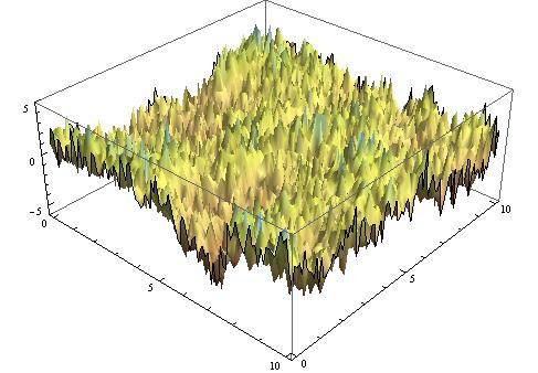
(a) Simulated realization of a stationary Gaussian random field with nugget effect.

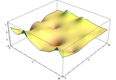
(b) Extrapolation by ordinary kriging for the field in Figure 5(a)

Fig. 5: Application of ordinary kriging to simulated data from Example 4

[scale=.30]Pictures/Variogram_summary.pdf

Fig. 6: Theoretical variogram (red), estimator (green) and fitted variogram (black) for the realization in Figure 5(a), compare Example 4

4 Extrapolation of Stable Random Fields

Let $X$ be an $\alpha$-stable random field having integral representation

$$X(t)=\int_{E}f_{t}(x)M(dx),\quad t\in\mathbb{R}^{d},$$ (23)

confer formula (10). For $\alpha\in(1,2]$, assume that the field $X$ is centered. If $\alpha\in(0,1]$, the mean value of $X$ does not exist.

We are looking for a predictor $\widehat{X}(t)$ of the value $X(t)$ at location $t\in\mathbb{R}^{d}$ based on the random vector $(X(t_{1}),\ldots,X(t_{n}))^{\top}$ in the form

$$\widehat{X}(t)=\sum_{i=1}^{n}\lambda_{i}X(t_{i}).$$ (24)

Let $T_{j}=\{t_{j,1},\ldots,t_{j,n_{j}}\}$, $j\in\mathbb{N}$ be a sequence of observation locations such that ${\rm dist}\,(T_{j},t)\to 0$ as $j\to\infty$ where ${\rm dist}\,(A,B)=\inf\{\|x-y\|:\;x\in A,\,y\in B\}$ is the Euclidean distance between two arbitrary sets $A,B\subset\mathbb{R}^{d}$. The predictor $\hat{X}_{j}(t)=\sum_{i=1}^{n_{j}}\lambda_{i}^{(j)}X(t_{j,i})$ is weakly consistent if $\hat{X}_{j}(t)\stackrel{{\scriptstyle\mathrm{\mathbf{P}}}}{{\mathop{\longrightarrow}\limits_{j\to\infty}}}X(t)$ for any $t\in\mathbb{R}^{d}$. It is stochastically continuous if $\hat{X}_{j}(s)\stackrel{{\scriptstyle\mathrm{\mathbf{P}}}}{{\mathop{\longrightarrow}\limits_{s\to t}}}\hat{X}_{j}(t)$ for any $j\in\mathbb{N}$ and $t\in\mathbb{R}^{d}$.

Let

$$\|f\|_{\alpha}=\left(\int_{E}|f(x)|^{\alpha}m(dx)\right)^{1/\alpha}$$ (25)

denote the norm of $f\in L^{\alpha}(E,m)$, $\alpha\geq 1$.

Theorem 4.1

Let the $\alpha$–stable random field $X$ in (23) be stochastically continuous, $\alpha\in(1,2]$. Let the predictor $\hat{X}_{j}$ defined above exist and be unique, exact and stochastically continuous for any $j\in\mathbb{N}$. Then $\hat{X}_{j}$ is weakly consistent.

Proof

Fix an arbitrary $t\in\mathbb{R}^{d}$. By (ST94, , Proposition 3.5.1), it is sufficient to show that $\sigma_{\hat{X}_{j}(t)-X(t)}\to 0$ as $j\to\infty$ to prove weak consistency. Let $s_{j}\in T_{j}$ be the point at which ${\rm dist}\,(s_{j},t)={\rm dist}\,(T_{j},t)$ for any $j\in\mathbb{N}$. It is clear that $s_{j}\to t$ as $j\to\infty$. Since $\hat{X}_{j}$ is exact it holds $\hat{X}_{j}(s_{j})=X(s_{j})$ for any $j$. Then we have

$$\sigma_{\hat{X}_{j}(t)-X(t)}=\|\sum_{i=1}^{n_{j}}\lambda_{i}^{(j)}f_{t_{j,i}}-f_{t}\|_{\alpha}\leq\|f_{s_{j}}-f_{t}\|_{\alpha}+\|\sum_{i=1}^{n_{j}}\lambda_{i}^{(j)}f_{t_{j,i}}-f_{{s_{j}}}\|_{\alpha}\to 0$$

as $j\to\infty$ by (ST94, , Proposition 3.5.1)), stochastic continuity of $X$ and $\hat{X}_{j}$ as well as exactness of $\hat{X}_{j}$.

4.1 Least Scale Predictor

For $\alpha\in(0,2]$, consider the following optimization problem

$$\sigma_{\widehat{X}(t)-X(t)}^{\alpha}=\int_{E}\left|f_{t}(x)-\sum_{i=1}^{n}\lambda_{i}f_{t_{i}}(x)\right|^{\alpha}m(dx)\,\to\,\min_{\lambda_{1},\ldots,\lambda_{n}}.$$ (26)

It is clear that the solution of the optimization problem (in case if it exists and is unique) will be an extrapolation. To see this, put $t=t_{j}$ and $\lambda_{i}(t_{j})=\delta_{ij}$, $i,j=1,\ldots,n$.

The predictor $\widehat{X}(t)$ based on a solution of this minimization problem is called least scale linear (LSL) predictor. This method is reminiscent of the least mean square error property (14) of the kriging.

If $\alpha\in(1,2]$ it is easy to see that any solution of the problem (26) is also a solution of the following system of equations

$$\int_{E}f_{t_{j}}(x)\left(f_{t}(x)-\sum_{i=1}^{n}\lambda_{i}f_{t_{i}}(x)\right)^{<\alpha-1>}m(dx)=0,\quad j=1,\ldots,n,$$ (27)

or equivalently

$$\left[X(t_{j}),X(t)-\sum_{i=1}^{n}\lambda_{i}X(t_{i})\right]_{\alpha}=0,\quad j=1,\ldots,n,$$ (28)

where $[\cdot,\cdot]_{\alpha}$ is the covariation, see Definition 16.

Exercise 23

Show that any solution of the problem (26) solves also the system of equations (27) or (28). Use the dominated convergence theorem.

Notice that equations in (26) are nonlinear in $\lambda_{1},\ldots,\lambda_{n}$ if $\alpha<2$ because the covariation is not linear in the second argument (cf. Section 2.4). Thus, numerical methods have to be applied to solve problem (26).

Properties of LSL predictor

Assume $1<\alpha\leq 2$. For the case $0<\alpha\leq 1$ see Section 4.4.

Theorem 4.2

The LSL predictor exists. If the random vector $\vec{X}=(X(t_{1}),\ldots,X(t_{n}))^{\top}$ is full–dimensional then the LSL predictor is unique.

Proof

We are using the properties of the best approximation in $L^{\alpha}(E,m)$-spaces for $1<\alpha\leq 2$. Let $L=span\{f_{t_{1}},\ldots,f_{t_{n}}\}$. This is a finite dimensional space. Denote for simplicity $f=f_{t}$ and $E(f)=\inf_{x\in L}\|f-x\|_{\alpha}$. Let us show that this infimum is attained in $L$.

Consider $\{x_{m}\}_{m\in\mathbb{N}}$ such that $x_{m}\in L$ $\forall m\in\mathbb{N}$ and $\|x_{m}-f\|_{\alpha}\to E(f)$ as $m\to\infty$. By the triangle inequality $\|x_{m}\|_{\alpha}\leq\|f\|_{\alpha}+\|f-x_{m}\|_{\alpha}$, so $\{x_{m}\}_{m\in\mathbb{N}}$ is a bounded sequence in a finite dimensional subspace. Thus, there exists a convergent subsequence $\{m_{j}\}_{j\in\mathbb{N}}$ and $f_{0}\in L$ such that $\|x_{m_{j}}-f_{0}\|_{\alpha}\to 0$ as $j\to\infty$. Since $\|f-x_{m_{j}}\|_{\alpha}\to\|f-f_{0}\|_{\alpha}$ and $\|f-x_{m_{j}}\|_{\alpha}\to E(f)$ as $j\to\infty$, it holds $E(f)=\|f-f_{0}\|_{\alpha}$. So $f_{0}$ is the best approximation.

For the proof of uniqueness, we use the strict convexity property. If $\alpha>1$ the space $L^{\alpha}(E,m)$ is strictly convex (see e.g. (DeVL93, , p. 59)), i.e. for all $g_{1},g_{2}\in L^{\alpha}(E,m)$ such that $\|g_{1}\|_{\alpha}=\|g_{2}\|_{\alpha}=1$, $g_{1}\neq g_{2}$ it follows $\|\beta g_{1}+(1-\beta)g_{2}\|_{\alpha}<1$ for any $\beta\in(0,1)$.

Take $y_{j}=\sum_{i=1}^{n}\lambda_{i}^{(j)}f_{t_{i}}\in L,$ $j=1,2$ such that $y_{1}\neq y_{2}$ and $\|f-y_{1}\|_{\alpha}=\|f-y_{2}\|_{\alpha}=E(f)$. Thus by strict convexity we have

$$E(f)\leq\left\|f-\frac{1}{2}\left(y_{1}+y_{2}\right)\right\|_{\alpha}=\left\|\frac{1}{2}\left(f-y_{1}\right)+\frac{1}{2}\left(f-y_{2}\right)\right\|_{\alpha}<E(f).$$

So we obtain a contradiction, and $y_{1}=y_{2}=f_{0}$. By the full–dimensionality of the random vector $\vec{X}$ and by Lemma 3 one can easily see that the set of the weights $\lambda_{i}$ in the representation $f_{0}=\sum_{i=1}^{n}\lambda_{i}f_{t_{i}}$ is unique.

Theorem 4.3 (KSS12 )

Let the stable random field $X$ in (23) be stochastically continuous. If the random vector $\vec{X}=\big{(}X(t_{1}),\ldots,X(t_{n})\big{)}^{\top}$ is full–dimensional then the LSL predictor is continuous.

4.2 Covariation Orthogonal Predictor

Throughout this Section, assume $\alpha\in(1,2]$. The linear predictor (24) with weights $\lambda_{1},\ldots,\lambda_{n}$ that are a solution of the system of equations

$$\left[X(t)-\sum_{i=1}^{n}\lambda_{i}X(t_{i}),X(t_{j})\right]_{\alpha}=0,\quad j=1,\ldots,n$$ (29)

is called Covariation Orthogonal Linear (COL) predictor. If the solution of (29) exists and is unique then it is an exact predictor, since we can put $\lambda_{i}(t_{j})=\delta_{ij}$, $i,j=1,\ldots,n$. This extrapolation method is reminiscent of the generic orthogonality property of simple kriging, cf. relation (20). It is also symmetric (in a sense) to the LSL predictor, compare the systems (28) and (29). In contrast to (28), the system (29) is linear which makes the computation of the weights $\lambda_{i}$ easier.

Introduce the covariation function $\kappa:\mathbb{R}^{d}\times\mathbb{R}^{d}\to\mathbb{R}$ of $X$ by

$$\kappa(s,t)=[X(s),X(t)]_{\alpha}.$$ (30)

Note that this function is not symmetric in its arguments, as opposed to the covariance function, cf. Definition 6.

By additivity of the covariation in the first argument (see Section 2.4), the system (29) rewrites as

$$\begin{pmatrix}\kappa(t_{1},t_{1})&\cdots&\kappa(t_{n},t_{1})\\ \vdots&\ddots&\vdots\\ \kappa(t_{1},t_{n})&\cdots&\kappa(t_{n},t_{n})\end{pmatrix}\begin{pmatrix}\lambda_{1}\\ \vdots\\ \lambda_{n}\end{pmatrix}=\begin{pmatrix}\kappa(t,t_{1})\\ \vdots\\ \kappa(t,t_{n})\end{pmatrix}.$$ (31)

If matrix $K=[\kappa(t_{i},t_{j})]_{i,j=1,\ldots,n}$ is positive definite the solution of this system exists and is unique.

For moving average and for sub–Gaussian fields $X$, sufficient conditions for the positive definiteness of $K$ can be given.

The COL Predictor for Moving Averages

Consider a moving average stable random field $X$ with representation

$$X(t)=\int_{\mathbb{R}^{d}}f(t-x)\,M(dx),\quad t\in\mathbb{R}^{d},$$

where $M$ is an $\alpha$–stable random measure with Lebesgue control measure and $f\in L^{\alpha}(\mathbb{R}^{d})$ (see Section 2.5 for the definition). By strict stationarity of $X$, it holds $[X(h),X(0)]_{\alpha}=[X(t+h),X(t)]_{\alpha}$ for all $t,\ h\in\mathbb{R}^{d}$. With slight abuse of notation, we write $\kappa(s-t)=[X(s-t),X(0)]_{\alpha}=\kappa(s,t)$, $s,t\in\mathbb{R}^{d}$ and the system of equations (31) is equivalent to

$$\begin{pmatrix}\kappa(0)&\cdots&\kappa(t_{n}-t_{1})\\ \vdots&\ddots&\vdots\\ \kappa(t_{n}-t_{1})&\cdots&\kappa(0)\end{pmatrix}\begin{pmatrix}\lambda_{1}\\ \vdots\\ \lambda_{n}\end{pmatrix}=\begin{pmatrix}\kappa(t-t_{1})\\ \vdots\\ \kappa(t-t_{n})\end{pmatrix}.$$ (32)

The next theorem gives a sufficient condition for the existence and uniqueness of the COL predictor.

Theorem 4.4

If the kernel $f:\mathbb{R}^{d}\to\mathbb{R}_{+}$ is a positive definite function that is positive on a set of non–zero Lebesgue measure then $\kappa$ is positive definite.

Proof

By formula (12), we have

$$\kappa(h)=\int_{\mathbb{R}^{d}}f(h-x)f^{\langle\alpha-1\rangle}(-x)\,dx,\quad h\in\mathbb{R}^{d}.$$

Thus for any $m\in\mathbb{N}$, $z_{1},\ldots,z_{m}\in\mathbb{R}$, $(z_{1},\ldots,z_{n})^{\top}\neq(0,\ldots,0)^{\top}$ and $s_{1},\ldots,s_{m}\in\mathbb{R}^{d}$ it holds

$$\sum_{i,j=1}^{m}\kappa(s_{i}-s_{j})z_{i}z_{j}=\int_{\mathbb{R}^{d}}\sum_{i,j=1}^{m}f(s_{i}-s_{j}-x)z_{i}z_{j}f^{\langle\alpha-1\rangle}(-x)\,dx>0.$$

An example of a process $X$ satisfying conditions of Theorem 4.4 is the $S\alpha S$ Ornstein–Uhlenbeck process: for any fixed $\lambda>0$

$$X(t)=\int_{\mathbb{R}}e^{-\lambda(t-x)}\mathbf{1}(t-x\geq 0)\,M(dx),\quad t\in\mathbb{R}.$$

By (ST94, , p. 138), we have $\widehat{X}(t)=e^{-\lambda(t-t_{n})}X(t_{n})$ if $t_{1}<\ldots<t_{n}<t$.

Theorem 4.5

If the covariation function $\kappa$ is positive definite and continuous then the COL predictor is continuous.

Proof

Since $\kappa$ is positive definite, matrix $K$ is invertible, and we have

$$\begin{pmatrix}\lambda_{1}(t)\\ \vdots\\ \lambda_{n}(t)\end{pmatrix}=\begin{pmatrix}\kappa(0)&\cdots&\kappa(t_{n}-t_{1})\\ \vdots&\ddots&\vdots\\ \kappa(t_{n}-t_{1})&\cdots&\kappa(0)\end{pmatrix}^{-1}\begin{pmatrix}\kappa(t-t_{1})\\ \vdots\\ \kappa(t-t_{n})\end{pmatrix}.$$

Since $\kappa$ is continuous, the weights $\lambda_{1},\ldots,\lambda_{n}$ are continuous in $t$.

Exercise 24

Show that continuous kernel functions with compact support yield a continuous covariation function $\kappa$. Use the dominated convergence theorem.

The COL Predictor for Gaussian and sub–Gaussian Random Fields

Let $X$ be a sub–Gaussian random field, i.e., $X(t)=A^{1/2}G(t)$, $t\in\mathbb{R}^{d}$ where $A\sim S_{\alpha/2}((\cos(\pi\alpha/4))^{2/\alpha},1,0)$ and $\boldsymbol{G}$ is a zero mean stationary Gaussian field independent of $A$. In (ST94, , Example 2.7.4), it is shown that for sub–Gaussian random fields, the covariation function is given by

$$\kappa(h)=2^{-\alpha/2}C(h)C(0)^{(\alpha-2)/2},\quad h\in\mathbb{R}^{d},$$ (33)

where $C(\cdot)$ is the covariance function of $G$.

It is easy to see that in this case the system (31) coincides with the simple kriging system (15) for $G$:

$$\begin{pmatrix}C(0)&\cdots&C(t_{n}-t_{1})\\ \vdots&\ddots&\vdots\\ C(t_{n}-t_{1})&\cdots&C(0)\end{pmatrix}\begin{pmatrix}\lambda_{1}\\ \vdots\\ \lambda_{n}\end{pmatrix}=\begin{pmatrix}C(t-t_{1})\\ \vdots\\ C(t-t_{n})\end{pmatrix}.$$ (34)

If $C$ is positive definite then the corresponding covariance matrix is invertible which ensures the existence and uniqueness of the solution of the system (34).

Theorem 4.6

If $(X(t_{1}),\ldots,X(t_{n}))^{\top}$ is full–dimensional and the covariance function $C$ of the Gaussian component is continuous then the COL predictor for sub–Gaussian random fields is continuous.

The proof is similar to the proof of Theorem 4.5.

Theorem 4.7

Let $1<\alpha\leq 2$. For Gaussian and sub–Gaussian random fields, the COL and LSL predictors coincide.

Proof

Introduce the notation $t_{0}=t$. Put $\lambda_{0}(t_{0})=-1$ and

$$\widehat{X}(t_{0})-X(t_{0})=A^{1/2}\sum_{i=0}^{n}\lambda_{i}(t_{0})G(t_{i}).$$

The characteristic function of random vector $(X(t_{0}),\ldots,X(t_{n}))^{\top}$ is given by

$$\mathbf{E}\exp\left\{i\sum_{k=0}^{n}\theta_{k}X(t_{k})\right\}=\exp\left\{-\left|\frac{1}{2}\sum_{i=0}^{n}\sum_{j=0}^{n}\theta_{i}\theta_{j}C(t_{i}-t_{j})\right|^{\alpha/2}\right\}$$ (35)

for all $\theta_{1},\ldots,\theta_{n}\in\mathbb{R}$, cf. (ST94, , Proposition 2.5.2). Now it is simple to see that

$$\sigma_{\widehat{X}(t_{0})-X(t_{0})}=\left(\frac{1}{2}\mathbf{v}\mathbf{a}\mathbf{r}\left(\sum_{i=0}^{n}\lambda_{i}(t_{0})G(t_{i})\right)\right)^{1/2}=\left(\frac{1}{2}\sum_{i,j=0}^{n}\lambda_{i}\lambda_{j}C(t_{i}-t_{j})\right)^{1/2}.$$

Thus, the LSL optimization problem is equivalent to

$$\sum_{i,j=0}^{n}\lambda_{i}\lambda_{j}C(t_{i}-t_{j})\to\min_{\lambda_{1},\ldots,\lambda_{n}}.$$

Taking derivatives we obtain $\sum_{j=0}^{n}C(t_{k}-t_{j})\lambda_{j}=0,$ $k=1,\ldots,n$ which coincides with the COL extrapolation system (34).

Remark 5

It follows from the proof of Theorem 4.7 (which is valid for all $\alpha\in(0,2)$) that the weights of the LSL predictor for sub–Gaussian random fields are a solution of the system (34) also in the case $\alpha\in(0,1]$. The statement of Theorem 4.6 holds as well. To summarize, the LSL predictor for stationary sub–Gaussian random fields $X$ exists and is unique and exact for all $\alpha\in(0,2]$ if the covariance function $C$ of the Gaussian component $G$ is positive definite. If $C$ is additionally continuous then this LSL predictor is also continuous.

4.3 Maximization of Covariation

In this section, we assume that $X$ is an $\alpha$–stable random field (23) with $\alpha\in(1,2]$. The predictor $\widehat{X}(t)=\sum_{i=1}^{n}\lambda_{i}(t)X(t_{i})$, whose weights $\lambda_{1}(t),\ldots,\lambda_{n}(t)$ solve the following optimization problem

$$\begin{cases}\left[\widehat{X}(t),X(t)\right]_{\alpha}=\sum_{i=1}^{n}\lambda_{i}(t)[X(t_{i}),X(t)]_{\alpha}\,\to\,\underset{\lambda_{1},\ldots,\lambda_{n}}{\max},\\ \sigma_{\widehat{X}(t)}=\sigma_{X(t)}\end{cases}$$ (36)

for $t\in\mathbb{R}^{d}$, is called Maximization of Covariation Linear (MCL) predictor.

The Lagrange function of the optimization problem (36) is given by

$$L(\vec{\lambda},\gamma)=\sum_{i=1}^{n}\lambda_{i}[X(t_{i}),X(t)]_{\alpha}+\gamma\left(\sigma^{\alpha}_{\sum_{i=1}^{n}\lambda_{i}X(t_{i})}-\sigma^{\alpha}_{X(t)}\right),\ \vec{\lambda}\in\mathbb{R}^{n},\ \gamma\in\mathbb{R}.$$

By taking partial derivatives and setting them equal to zero, we get

$$\begin{cases}[X(t_{j}),X(t)]_{\alpha}+\gamma\cdot\partial\sigma^{\alpha}_{\sum_{i=1}^{n}\lambda_{i}X(t_{i})}/\partial\lambda_{j}=0,\quad j=1,\ldots,n,\\ \sigma_{\sum_{i=1}^{n}\lambda_{i}X(t_{i})}=\sigma_{X(t)}.\end{cases}$$ (37)

Analogously to formula (28) one can obtain

$$\frac{\partial\sigma^{\alpha}_{\sum_{i=1}^{n}\lambda_{i}X(t_{i})}}{\partial\lambda_{j}}=\alpha\cdot\left[X(t_{j}),\sum_{i=1}^{n}\lambda_{i}(t)X(t_{i})\right]_{\alpha}.$$

Since $\gamma=-1/\alpha$, $\lambda_{i}(t_{j})=\delta_{ij}$ is obviously a solution of system (37) for $t=t_{j}$, $j=1,\ldots,n$, the MCL predictor is exact.

Let us discuss the properties of the MCL predictor. Notice that here no direct analogy with kriging can be drawn. For instance, a counterpart $\sigma_{\widehat{X}(t)}\leq\sigma_{X(t)}$ of the shrinkage property (18) is deliberately mutated to the additional condition $\sigma_{\widehat{X}(t)}=\sigma_{X(t)}$. The reason for this is that both conditions lead to the same solutions due to the convexity of the optimization problem (36).

Introduce the following notation: $\zeta(t)=(\kappa(t_{1},t),\ldots,\kappa(t_{n},t))^{\top},$ $t\in\mathbb{R}^{d},$ the function $\sigma_{0}:\mathbb{R}^{d}\to\mathbb{R}_{+}$ is $\sigma_{0}(t)=\sigma_{X(t)}=\kappa(t,t)$. The function $\Psi:\mathbb{R}^{n}\to\mathbb{R}_{+}$ is defined by

$$\Psi(\lambda)=\sigma_{\widehat{X}(t)}=\left\|\sum_{i=1}^{n}\lambda_{i}f_{t_{i}}\right\|_{\alpha}.$$

Denote the level set of function $\Psi$ at level $u\in\mathbb{R}$ by $B_{u}=\{\lambda\in\mathbb{R}^{n}:\Psi(\lambda)\leq u\}.$ The support set of any convex set $B\subset\mathbb{R}^{n}$ at a point $x\in\mathbb{R}^{n}$ is defined by

$$T(B,x)=\left\{y\in B:\langle y,x\rangle=\sup_{z\in B}\langle z,x\rangle\right\}.$$

It is known that for strictly convex sets $B$ and any non–zero $x\in\mathbb{R}^{n}$ the support set $T(B,x)$ is a singleton. We denote this single point by $y_{B,x}$.

Theorem 4.8

Assume that the $\alpha$-stable random vector $X=(X(t_{1}),\ldots,X(t_{n}))^{\top}$ is full–dimensional.

1. The solution of the optimization problem (36) exists for all $t\in\mathbb{R}^{d}$. If $\kappa(t_{i},t)\neq 0$ for some $i=1,\ldots,n$ then the MCL predictor $\widehat{X}(t)$ is unique.

2. If $\kappa$ is a continuous function on $\mathbb{R}^{d}\times\mathbb{R}^{d}$ and $\kappa(t_{i},t)\neq 0$ for some $i=1,\ldots,n$ then the MCL predictor is continuous in $t$.

Proof

For the proof of the existence and uniqueness of MCL we refer the reader to the paper KSS12 . It is also shown there that the vector of MCL weights

$$\lambda(t)=(\lambda_{1}(t),\ldots,\lambda_{n}(t))^{\top}$$

is equal to $y_{B_{\sigma_{0}(t)},\zeta(t)}$ for any $t\in\mathbb{R}^{d}$ whereas the set $B_{\sigma_{0}(t)}$ is strictly convex. Let us prove that $\lambda:\mathbb{R}^{d}\to\mathbb{R}^{n}$ is a continuous function. It is easy to see that $B_{\sigma_{0}(t)}=\frac{1}{\sigma_{0}(t)}B_{1}$, because the sets $B_{\sigma_{0}(t)}$, $t\in\mathbb{R}^{d}$ are homothetic, i.e. $aB_{\sigma_{0}(t)}=B_{\sigma_{0}(t)/a}$, $a>0$. Thus by simple geometric considerations

$$T(B_{\sigma_{0}(t)},\zeta(t))=T\left(\frac{1}{\sigma_{0}(t)}B_{1},\zeta(t)\right)=\frac{1}{\sigma_{0}(t)}T(B_{1},\zeta(t)),$$

thus $\lambda(t)=\frac{1}{\sigma_{0}(t)}y_{B_{1},\zeta(t)}$. Put $B=B_{1}$ and $x(s)=y_{B,\zeta(s)}$ for any $s\in\mathbb{R}^{d}$. Show that $\lim_{s\to t}x(s)=x(t)$. This limit exists by the definition of the support set and continuity of the scalar product. We know that $\zeta(s)\to\zeta(t)$ as $s\to t$ since $\kappa$ is a continuous function. Moreover, $B$ is a compact, and $x(s)\in B$ for all $s$. Choose a convergent sequence $s_{m}\to t$ as $m\to\infty$ such that $x(s_{m})\to y$ as $m\to\infty$, where $y\in B$. Show that $y=x(t)$. It is clear that $\langle x(s_{m}),\zeta(s_{m})\rangle\to\langle y,\zeta(t)\rangle$ as $m\to\infty$. And for any $x\in B$ it holds

$$\langle x,\zeta(t)\rangle=\lim_{m\to\infty}\langle x,\zeta(s_{m})\rangle\leq\lim_{m\to\infty}\langle x(s_{m}),\zeta(s_{m})\rangle=\langle y,\zeta(t)\rangle.$$

The inequality here is due to the fact that $\{x(s_{m})\}=T(B,\zeta(s_{m}))$ for any $m\in\mathbb{N}$. Thus $y=y_{B,\zeta(t)}$.

4.4 Case $\alpha\in(0,1]$

As noticed in Section 2.4, the covariation function is not defined for $\alpha\in(0,1]$. Moreover, the function $\|\cdot\|_{\alpha}$ for $\alpha<1$ defined in (25) is not a norm anymore since the triangle inequality fails to hold. The property of strict convexity of $L^{\alpha}(E,m)$ does not hold as well.

To cope with these drawbacks, one may come to an idea that the codifference (cf. Definition 17) can be used instead of the covariation in COL and MCL methods. However, it does not seem to make advances in extrapolation. For instance, replacing the covariation by the codifference in the MCL method leads to the optimization problem

$$\begin{cases}\tau(\widehat{X}(t),X(t))=\sigma_{\widehat{X}(t)}+\sigma_{X(t)}-\sigma_{\widehat{X}(t)-X(t)}\ \to\ \max\limits_{\lambda_{1},\ldots,\lambda_{n}}\\ \sigma_{\widehat{X}(t)}=\sigma_{X(t)}.\end{cases}$$ (38)

Using the constraint $\sigma_{\widehat{X}(t)}=\sigma_{X(t)}$, the first relation rewrites

$$\tau(\widehat{X}(t),X(t))=2\sigma_{X(t)}-\sigma_{\widehat{X}(t)-X(t)}.$$

Hence, the method (38) is equivalent to LSL extrapolation, i.e., to minimizing the scale parameter

$$\sigma_{\widehat{X}(t)-X(t)}=\|f_{t}-\sum_{i=1}^{n}\lambda_{i}f_{t_{i}}\|_{\alpha}$$

of $\widehat{X}(t)-X(t)$.

Replacing the covariation by the codifference in the COL method (29), one arrives at the system of nonlinear equations

$$\tau_{\widehat{X}(t),X(t_{i})}=\tau_{X(t),X(t_{i})},\ \ \ i=1,\ldots,n.$$ (39)

Here the numerical computation of a solution is necessary, which can be very time consuming. Furthermore, it is shown in Hagel12 that the solution of the system (39) is not unique. For this reason, we shall not pursue the method (39) in future.

Neither leads the maximization of $\tau_{\widehat{X}(t),X(t)}$ with respect to weights $\lambda_{1},\ldots,\lambda_{n}$ to a unique predictor (24). In particular, its existence is not really clear. As an example consider a random field (23) with the kernel function $f_{t}$ of compact support such that the supports of $f_{t}$ and $f_{t_{1}},\ldots,f_{t_{n}}$ do not overlap. Then it is easy to see that $\tau_{\widehat{X}(t),X(t)}=0$ allowing for an arbitrary choice of weights $\lambda_{1},\ldots,\lambda_{n}$.

In the remainder of this Section, we focus on the properties of the LSL method for $\alpha$–stable random fields with $\alpha\in(0,1]$. First of all, the fundamental question of existence has to be answered. Here we follow Hagel12 and do this in a more general setting of $r$–normed vector spaces.

Definition 19

Let $V$ be a vector space over a field $\mathbb{K}$. A map $||.||_{(r)}:V\rightarrow\mathbb{R}_{+}$ is called an $r$–norm, if there exists $K\geq 1$ and $r>0$ such that

$$||x||_{(r)} =0\Leftrightarrow x=0,$$

$$||ax||_{(r)} =|a|\cdot||x||_{(r)}\ \ \ \forall\ a\in\ \mathbb{K},\ \forall\ x\ \in\ V,$$

$$||x+y||_{(r)} \leq K(||x||_{(r)}+||y||_{(r)})\ \ \ \forall\ x,y\ \in\ V,$$

$$||x+y||_{(r)}^{r} \leq||x||_{(r)}^{r}+||y||_{(r)}^{r}\ \ \ \forall\ x,y\ \in\ V.$$

Now the existence theorem can be formulated.

Theorem 4.9 (Hagel12 )

Let $V$ be a vector space over $\mathbb{R}$ with r-norm $||\cdot||_{(r)}$ and let $f_{1},\ldots,f_{n}\in V$ be linearly independent. For any $f_{0}\in V$, there exist real numbers $\lambda_{1}^{*},\ldots,\lambda_{n}^{*}$ such that

$$||f_{0}-\sum_{i=1}^{n}\lambda_{i}^{*}f_{i}||_{(r)}=\inf\limits_{\lambda_{1},\ldots,\lambda_{n}\in\mathbb{R}}||f_{0}-\sum_{i=1}^{n}\lambda_{i}f_{i}||_{(r)}.$$

If we set $V=L^{\alpha}(E,m)$ and note that $||\cdot||_{(\alpha)}=\|\cdot\|_{\alpha}$ defined in (25) is an $\alpha$-norm on $L^{\alpha}(E,m)$ (even a norm if $\alpha\geq 1$), the existence of the LSL predictor follows immediately from Theorem 4.9. In contrast to the case $\alpha\in(1,2]$ (Theorem 4.2), the uniqueness of the LSL weights $\lambda^{*}:=(\lambda_{1}^{*},\ldots,\lambda_{n}^{*})^{\top}$ in Theorem 4.9 is not guaranteed. We illustrate this by the following example. Introduce the notation $H_{\alpha}(\lambda)=\sigma_{\widehat{X}(t)-X(t)}$ for $\lambda=(\lambda_{1},\ldots,\lambda_{n})^{\top}\in\mathbb{R}^{n}$.

Example 5

Consider the measurable space $(E,m)=([0,1],\nu_{1})$ and the kernel function $f_{t}(x)=\mathbf{1}\left(x\in(t+\frac{1}{4},t+\frac{3}{4})\right)$. Given $t_{1}=\frac{1}{4}$, predict the value of the symmetric $\alpha$–stable process $X(t)=\int\limits_{[0,1]}f_{t}(x)\,M(dx)$ at the point $t=0$. By elementary calculations we obtain

$$H_{\alpha}^{\alpha}(\lambda)=\int\limits_{[0,1]}|f_{t}(x)-\lambda f_{t_{1}}(x)|^{\alpha}dx=\frac{1}{4}(1+|1-\lambda|^{\alpha}+|\lambda|^{\alpha}).$$

It is easy to see that for $0<\alpha<1$, $H_{\alpha}$ has two global minima at $\lambda=0$ and $\lambda=1$. If $\alpha=1$ the set of all global minimum points equals the interval $[0,1]$. For values $\alpha>1$, the function $H_{\alpha}$ has a unique global minimum at $\lambda=0.5$.

In order to get unbiased prediction (provided that the first moment of $X$ is finite), the parameter space is often restricted to $\{(\lambda_{1},\ldots,\lambda_{n})^{\top}\in\mathbb{R}^{n}:\ \ \sum_{i=1}^{n}\lambda_{i}=1\}$. S. Hagel showed in Hagel12 that this restriction does not cause uniqueness of LSL prediction for $\alpha\in(0,1)$. Alternatively, the following algorithmic approach to choose a unique global minimum in the LSL optimization problem is proposed:

Algorithm 1

Let $\{X(t),\;t\in T\}$ be an $\alpha$–stable random field (23) with $0<\alpha<1$ and $T\subset\mathbb{R}^{d}$. Let $t_{1},\ldots,t_{n}\in T$ be fixed such that functions $f_{t_{1}},\ldots,f_{t_{n}}$ are linearly independent.

1. Order the points $t_{1},\ldots,t_{n}$ so that

   $$\|t-t_{1}\|\leq\|t-t_{2}\|\leq\ldots\leq\|t-t_{n}\|$$

   and if $\|t-t_{i}\|=\|t-t_{i+1}\|$ for some $i\in\{1,\ldots,n-1\}$ then

   $$t_{i}^{(p)} =t_{i+1}^{(p)}\ \ \ \ \mbox{for all }p=1,\ldots,k-1$$ (40)

   $$t_{i}^{(k)} <t_{i+1}^{(k)}$$ (41)

   for some $k\in\{1,\ldots,m\}$, where $t_{i}^{(p)}$ is the $p$–th component of $t_{i}$.

2. Determine the set $A_{0}$ of all critical points

   $$A_{0}=\{(\lambda_{1},\ldots,\lambda_{n})\in\mathbb{R}^{n}\ \text{:}\ \ H_{\alpha}(\lambda_{1},\ldots,\lambda_{n})=\inf\limits_{(\mu_{1},\ldots,\mu_{n})\in\mathbb{R}^{n}}H_{\alpha}(\mu_{1},\ldots,\mu_{n})\}$$

3. Reduce $A_{0}$ step by step to sets $A_{1}\supseteq A_{2}\supseteq\dots\supseteq A_{n}$ given by

   $$A_{j}=\{(\lambda_{1},\ldots,\lambda_{n})\in A_{j-1}\ \text{:}\ \ \lambda_{j}=\max\limits_{(\mu_{1},\ldots,\mu_{n})\in A_{j-1}}\mu_{j}\},\ \ \ \ \ j=1,\ldots,n.$$

Clearly, the set $A_{n}$ consists of just one element.

Definition 20

We call $\widehat{X}(t)=\sum_{i=1}^{n}\lambda_{i}^{*}X(t_{i})$ the best LSL predictor if $(\lambda_{1}^{*},\ldots,\lambda_{n}^{*})\in A_{n}$.

The above construction has a simple intuitive meaning. The points $t_{1},\ldots,t_{n}$ are ordered with respect to their distance to $t$. To get a unique ordering, conditions (40) and (41) are required. Points with a smaller distance to $t$ are regarded to exert more influence on the value of $X$ at $t$, so their weights should be maximized first.

To show that $A_{j}\neq\emptyset$, $j=1,\dots,n$ we notice that $A_{0}$ is nonempty and compact. Therefore, the projection mapping $(x_{1},\ldots,x_{n})\mapsto x_{1}$ takes its maximum on $A_{0}$. Hence, $A_{1}$ is nonempty and compact as well. Sets $A_{2},\ldots,A_{n}$ are not empty by induction.

It can be easily proved that the best LSL predictor is exact. To see this, let $t=t_{i}$ for some $i\in\{1,\ldots,n\}$ and let $t_{1},\ldots,t_{n}\in\mathbb{R}^{d}$ be as in Algorithm 1. Relations (40) and (41) then imply that $t=t_{1}$. Trivially $(1,0,\ldots,0)\in A_{0}$ holds. Due to the linear independence of $f_{t_{1}},\ldots,f_{t_{n}}$, it holds that $A_{n}=A_{0}=\{(1,0,\ldots,0)\}$.

For $1<\alpha\leq 2$, Theorem 4.3 stated the continuity of LSL prediction. In contrast, the best LSL predictor is not necessarily continuous for $0<\alpha\leq 1$ as the next example shows.

Example 6

Let $X=\{X(t),\;t\in\mathbb{R}^{2}\}$ be an $\alpha$–stable random field (23) with $0<\alpha<1$, $f_{t}(x)=\mathbf{1}\left(x\in(\min\{t^{(1)},t^{(2)}\},\max\{t^{(1)},t^{(2)}\})\right)$ for $t=(t^{(1)},t^{(2)})\in\mathbb{R}^{2}$, $E=\mathbb{R}$ and $M$ being a $S\alpha S$ random measure on $\mathbb{R}$ with Lebesgue control measure. It follows from relations (8), (9) and Markov inequality that that $X$ is stochastically continuous, i.e., it has a.s. no jumps at fixed locations $t$. For $n=1$, introduce $t_{0}=(\frac{1}{2},\frac{3}{2})$, $t_{1}=(0,1)$, $t=t_{0}+\varepsilon$, where $\varepsilon=(\delta,\delta)\in\mathbb{R}^{2}$ for some $\delta\in(-\frac{1}{2},\frac{1}{2})$. Consider the best LSL predictor $\widehat{X}(t)$ of $X(t)$ based on the data $X(t_{1})$. It holds

$$H_{\alpha}^{\alpha}(\lambda) =\int\limits_{\mathbb{R}}|f_{t_{0}+\epsilon}(x)-\lambda f_{t_{1}}(x)|^{\alpha}dx$$

$$=\left(\frac{1}{2}+\delta\right)\cdot|\lambda|^{\alpha}+\left(\frac{1}{2}-\delta\right)\cdot|1-\lambda|^{\alpha}+\left(\frac{1}{2}+\delta\right).$$

If $\delta>0$ then $H_{\alpha}$ has a global minimum at $\lambda=0$ and if $\delta<0$ it has a global minimum at $\lambda=1$. So $\widehat{X}(t)$ is discontinuous at $t=t_{0}$.

In addition to the best LSL prediction, it is possible to treat the case $\alpha=1$ similar to the case $1<\alpha<2$. The following approach is proposed in Hagel12 . For a symmetric $1$–stable field $\{X(t)\ \text{:}\ t\in T\}$ with integral representation

$$X(t)=\int\limits_{E}f_{t}(x)\,M(dx)$$

let the function $f_{t}\in L^{1}(E,\mathcal{E},m)\cap L^{\delta}(E,\mathcal{E},m)$ for some $\delta>1$. Then we have

$$\int\limits_{E}|f_{t}(x)-\sum_{i=1}^{n}\lambda_{i}f_{t_{i}}(x)|^{\gamma}m(dx)<\infty$$

for all $\gamma\in[1,\delta]$, $\lambda_{1},\ldots,\lambda_{n}\in\mathbb{R}$ and $t,t_{1},\ldots,t_{n}\in T$. Now fix $t,t_{1},\ldots,t_{n}\in T$ and chose an arbitrary sequence $(\gamma_{k})_{k\in\mathbb{N}}\subset(1,\delta]$ which converges to $1$ as $k\to\infty$. Let $(\lambda_{1}^{(\gamma_{k})},\ldots,\lambda_{n}^{(\gamma_{k})})$ be the unique solution of

$$\int\limits_{E}|f_{t}(x)-\sum_{i=1}^{n}\lambda_{i}f_{t_{i}}(x)|^{\gamma_{k}}m(dx)\rightarrow\min_{\lambda_{1},\ldots,\lambda_{n}}.$$ (42)

Applying the stability theorem in (Kos91, , p.225) it follows the convergence

$$\int\limits_{E}|f_{t}(x)-\sum_{i=1}^{n}\lambda_{i}^{(\gamma_{k})}f_{t_{i}}(x)|^{\gamma_{k}}m(dx)\rightarrow\inf_{\mu_{1},\ldots,\mu_{n}}\int\limits_{E}|f_{t}(x)-\sum_{i=1}^{n}\mu_{i}f_{t_{i}}(x)|m(dx)$$ (43)

as $k\to\infty.$ Moreover, it can be shown that

$$(\lambda_{1}^{(\gamma_{k})},\ldots,\lambda_{n}^{(\gamma_{k})})\rightarrow(\lambda_{1}^{*},\ldots,\lambda_{n}^{*}),\quad k\rightarrow\infty.$$

This set of weights $(\lambda_{1}^{*},\ldots,\lambda_{n}^{*})$ exists and is unique if all LSL prediction problems (42) with stability indices $\gamma_{k}>1$ do so. It also does not depend on the choice of the sequence $(\gamma_{k})_{k\in\mathbb{N}}\subset(1,\delta]$ such that $\gamma_{k}\to 1$ as $k\to\infty$.

Definition 21

The predictor $\widehat{X}^{*}(t)=\sum_{i=1}^{n}\lambda_{i}^{*}X(t_{i})$, $t\in T$ is called an index–continuous LSL predictor (ICLSL) for the symmetric $1$–stable random field $X$.

It is still an open problem to explore the statistical properties of ICLSL.

4.5 Numerical Examples

In this section, LSL, COL and MCL extrapolation methods (as well as Maximum Likelihood extrapolation and conditional simulation for sub–Gaussian random fields) are applied to simulated data of various $\alpha$–stable random processes and fields $X$ for $\alpha\in(0,2)$.

The random fields are simulated and extrapolated on an equidistant $50\times 50$ –grid of points within $T=[0,1]^{2}$. In Examples 1 and 2, the simulated field $X=\{X(t),\;t\in[0,1]^{2}\}$ is observed at the points $t_{1},\ldots,t_{16}$ given by their coordinates

$$t_{1} =(0,0), t_{2} =(0,0.3), t_{3} =(0,0.6), t_{4} =(0,0.9),$$

$$t_{5} =(0.3,0), t_{6} =(0.3,0.3), t_{7} =(0.3,0.6), t_{8} =(0.3,0.9),$$

$$t_{9} =(0.6,0), t_{10} =(0.6,0.3), t_{11} =(0.6,0.6), t_{12} =(0.6,0.9),$$

$$t_{13} =(0.9,0), t_{14} =(0.9,0.3), t_{15} =(0.9,0.6), t_{16} =(0.9,0.9).$$

1. Sub–Gaussian Random Fields

Consider a stationary sub–Gaussian random field $X$ described in Example 5 of Section 2.5 with $\alpha=1.2$. The Gaussian part $G$ of this field has a Whittle–Matérn covariance function (cf. Section 2.2, Example 6) with parameters as in Figure 1(a). Figure 7(a) shows a realization of $X$. The corresponding LSL (coinciding with COL by Theorem 4.7) and MCL predictors can be seen in Figures 7(b) and 7(c). Both predictions are smoother than the realization of the field itself. Since predictions in Figures 7(b) and 7(c) look quite similar and can not be told one from another by eye, their difference is given in Figure 7(d).

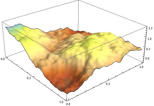
(a) Realization of a sub–Gaussian random field with $\alpha=1.2$.

(b) Corresponding LSL (COL) predictor

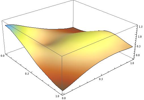
(c) Corresponding MCL predictor

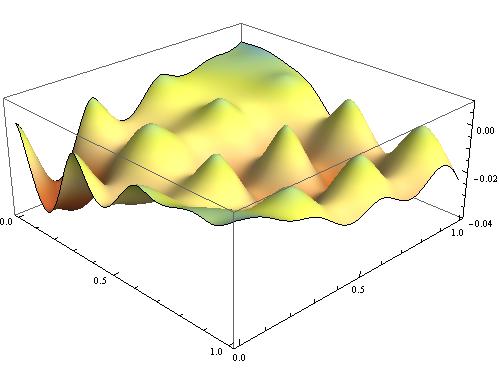
(d) Pointwise difference ((b)-(c)) between LSL (b) and MCL (c) predictors

Fig. 7: Realization of a sub–Gaussian random field for $\alpha>1$ and different predictors

Figure 8(a) shows a realization of the stationary sub–Gaussian field with $\alpha=0.8$ and covariance function $C$ of the Gaussian part as above. A Maximum Likelihood (ML) predictor for sub–Gaussian random fields is introduced in KSS12 . It is shown in Theorem 11 of that paper that LSL, COL and ML methods coincide if $\alpha\in(1,2)$. However, its proof does not depend on $\alpha$ covering (with regard to Remark 5 of this chapter) the range of all $\alpha\in(0,2)$. Thus, LSL and ML predictors coincide for sub–Gaussian random fields with any stability index $\alpha\in(0,2)$. A possibility of extrapolation of sub–Gaussian random fields $X$ by conditional simulation (CS) of the Gaussian component $G$ of $X$ and the subsequent scaling by $\sqrt{A}$ is straightforward; see e.g. Pai98 and (Karcher12, , p. 112). Algorithms for the conditional simulation of $G$ are given in Lan02 . Corresponding extrapolation results for LSL (ML) and CS methods are given in Figures 8(b) and 8(c). Notice that the ML prediction for this realization of $X$ is much smoother than CS prediction.

(a) Realization of a sub–Gaussian random field with $\alpha=0.8$.

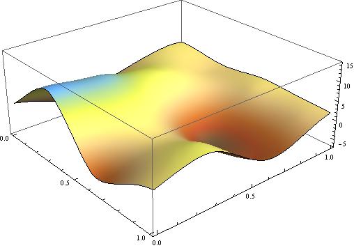
(b) Corresponding LSL (ML) predictor

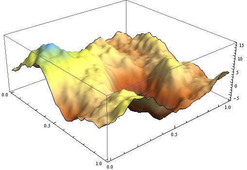
(c) Prediction by conditional simulation

Fig. 8: Realization of a sub–Gaussian random field for $\alpha<1$ and different predictors

2. Skewed stable Lévy Motion

Consider the two–dimensional $1.5$–stable Lévy motion $X$ defined by

$$X(t)=\int_{0}^{1}\int_{0}^{1}\mathbf{1}(x_{1}\leq t_{1},x_{2}\leq t_{2})\,M\big{(}d(x_{1},x_{2})\big{)},\quad t=(t_{1},t_{2})^{\top}\in[0,1]^{2},$$

where $M$ is a non–symmetric centered $1.5$–stable random measure with skewness intensity $\beta=1$. Comparing a realization of $X$ (Figure 9(a)) with its LSL, COL and MCL predictors (Figures 9(b), 9(c) and 9(d)) one can see that prediction has a smoothing effect.

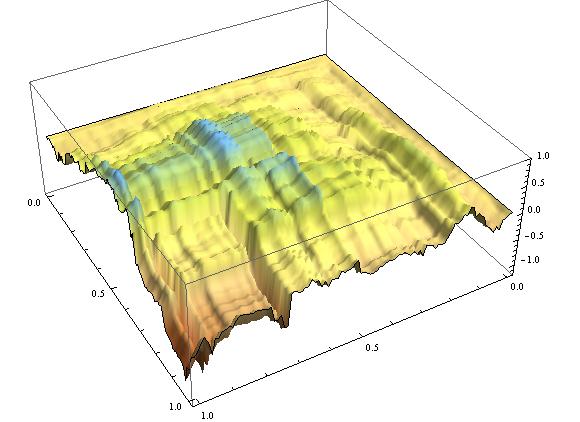
(a) Realization of stable Lévy motion with skewness intensity $\beta=1$ and $\alpha=1.5$

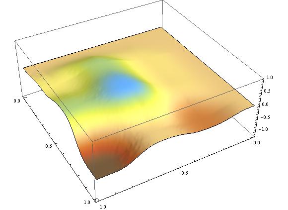
(b) Corresponding LSL predictor

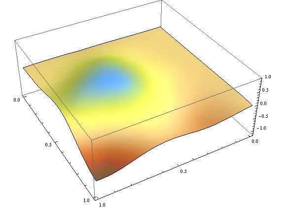
(c) Corresponding COL predictor

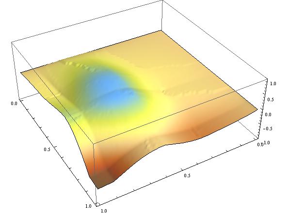
(d) Corresponding MCL predictor

Fig. 9: Realization of a skewed stable Lévy motion field and different predictors

3. Stable Ornstein–Uhlenbeck Process

Let $X$ be a $1.6$-stable Ornstein–Uhlenbeck process with $\lambda=0.5$ defined in Example 2 of Section 2.5. Figure 4.5 shows a trajectory of this process and different interpolators. The process $X$ is observed at positions $t_{i}=1,\dots,10$ within $[0,10]$. It can be seen that LSL interpolation is very smooth. In contrast, the COL predictor is piecewise smooth and continuous on the whole interval.

A trajectory (black) of the stable Ornstein–Uhlenbeck process together with LSL (red), COL (green) and MCL (blue) predictors, $\alpha=1.6$

4. Stable Moving Average

Let $X=\{X(t),\ t\in[0,0.49]^{2}\}$ be a moving average field (cf. Example 2 of Section 2.5) with the kernel function

$$f(x)=0.5\left(0.04-\|x\|^{2}\right)\mathbf{1}\left(\|x\|\leq 0.2\right),$$

stability index $\alpha=0.5$ and skewness intensity $\beta=0.8$. Random field $X$ is simulated on an equidistant $50\times 50$–grid of points within $[0,0.49]^{2}$ using the step function approach from paper KSS13 with an accuracy ($L^{\alpha}$-error) $\epsilon=0.01$. The field is observed at points

$$t_{1} =(0,0), t_{2} =(0,0.25), t_{3} =(0,0.49),$$

$$t_{4} =(0.25,0), t_{5} =(0.25,0.25), t_{6} =(0.25,0.49),$$

$$t_{7} =(0.49,0), t_{8} =(0.49,0.25), t_{9} =(0.49,0.49).$$

To solve the optimization problems for the best LSL prediction (cf. Section 4.4) numerically, an average of $8$ realizations of the simulated annealing algorithm from Kirkpatrick1983 is used. Figures 10(a) and 10(b) show a realization of $X$ and its best LSL predictor. The numerical optimization procedure is quite time consuming with $136$ min. of computation time (Pentium Dual Core E5400, $2.70$ GHz, $8$ GB RAM) per extrapolation.

(a) Realization of a skewed $0.5$–stable moving average random field

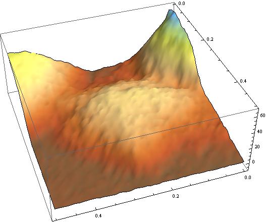
(b) Corresponding best LSL predictor

Fig. 10: Realization of a skewed moving average field with $\alpha=0.5$ and its best LSL predictor

5 Open problems

In contrast to kriging methods, there is no common methodology of measuring prediction errors in the stable case. We propose the following measures

$$\sup_{t\in\mathbf{R}^{d}}\left(\mathbf{E}|X(t)-\widehat{X}(t)|^{p}\right)^{1/p}=c_{\alpha}(p)\sup_{t\in\mathbf{R}^{d}}\|f_{t}-\sum_{i=1}^{n}\lambda_{i}f_{t_{i}}\|_{\alpha},$$ (44)

where $1<p<\alpha$ and $c_{\alpha}(p)>0$ is a constant from relation (8), or

$$\mathbf{P}\left(\sup_{t\in\mathbf{R}^{d}}|X(t)-\widehat{X}(t)|>\epsilon\right),\quad\epsilon>0.$$ (45)

It is an open problem to find lower and upper bounds for these errors as well as minimax bounds where the infimum over a subclass of stable random fields $X$ is additionally considered in relations (44) and (45). Alternatively, one can be interested in the asymptotic behavior of $\mathbf{P}\left(\sup_{t\in\mathbf{R}^{d}}|X(t)-\widehat{X}(t)|<\epsilon\right)$ as $\epsilon\to 0$ which is related to small deviation problems.