A PSO Approach for Optimum Design of Multivariable PID Controller for nonlinear systems

Abstract

The aim of this research is to design a PID Controller using particle swarm optimization (PSO) algorithm for multiple-input multiple output (MIMO) Takagi-Sugeno fuzzy model. The conventional gain tuning of PID controller (such as Ziegler-Nichols (ZN) method) usually produces a big overshoot, and therefore modern heuristics approach such as PSO are employed to enhance the capability of traditional techniques. However, due to the computational efficiency, only PSO will be used in this paper. The results show the advantage of the PID tuning using PSO-based optimization approach.

I Introduction

PID control, which is usually known as a classical output feedback control for SISO systems, has been widely used in the industrial world [1] and [2]. The tuning methods of PID control are adjusting the proportional, the integral and the derivative gains to make an output of a controlled system track a target value properly. several researchers focus on multiple-input multiple output MIMO control systems. Because many industrial processes are MIMO systems which need MIMO control techniques to improve performance, though they are naturally more difficult than SISO systems. As we know, MIMO PID controller design has developed over a number of years. Luyben (1986) proposed a simple tuning method for decentralized PID controllers in MIMO system from single-loop relay tests [3]. Yusof and Omatu (1993) presented a multivariable self-tuning PID controller based on estimation strategies [4]. Wang et al. (1997) proposed a tuning method for fully cross-coupled multivariable PID controller from decentralized relay feedback test to find the critical oscillation frequency of the system by first designing the diagonal elements of multivariable PID controller independent of off-diagonal ones [5]. Recently, the computational intelligence has proposed particle swarm optimization (PSO) [6,7] as opened paths to a new generation of advanced process control. The PSO algorithm, proposed by Kennedy and Eberhart [6] in 1995, was an evolution computation technology based on population intelligent methods. In comparison with genetic algorithm, PSO is simple,easy to realize and has very deep intelligent background. It is not only suitable for scientific research, but also suitable for engineering applications in particular. Thus, PSO received widely attentions from evolution computation field and other fields. Now the PSO has become a hotspot of research. Various objective functions based on error performance criterion are used to evaluate the performance of PSO algorithms.

In this paper, a scheduling PID tuning parameters using particle swarm optimization strategy for MIMO nonlinear systems . This paper has been organized as follows: In section 2, a brief review of the TS fuzzy model formulation is given. Estimation method of recursive weighted least-squares (RWLS)in section 3. In section 4, PID control systems of multivariable processes. Finally, some conclusions are made in section 5.

II Takagi-Sugeno fuzzy model of a MIMO process

Generally, modeling process consists to obtain a parametric model with the same dynamic behavior of the real process. In this section, we are interested to the problem of the MIMO process identification[8]. We consider a MIMO system with $n_{i}$ inputs and $n_{0}$ outputs. The MISO models are a input-output NARX (Non linear Auto Regressive with eXogenous input) defined by:

$$y_{l}(k+1)=f_{l}(x_{l}(k))\,\,\,\,\,\,\,\,\,\,l=1,2,...,n_{0}$$ (1)

With the regression vector represented by:

$$\begin{array}[]{c}x_{l}(k)=[\{y_{1}(k)\}_{0}^{n_{yl1}},\{y_{2}(k)\}_{0}^{n_{yl2}},...,\{y_{n0}(k)\}_{0}^{ln_{yln_{0}}},\\ \,\,\,\,\,\,\,\,\,\,\,\,\,\{u_{1}(k)\}_{n_{dl1}}^{n_{ul1}},\{u_{2}(k)\}_{n_{dl2}}^{n_{ul2}},...,\{u_{n_{i}}(k)\}_{n_{dln_{i}}}^{n_{ud1n_{i}}}]\end{array}$$ (2)

$n_{y}$ and $n_{u}$ define the number of delayed outputs and inputs respectively. $n_{d}$ is the number of pure delays. $n_{y}$ is a $n_{0}*n_{0}$ matrix and $n_{u}$, $nd$ are $n_{0}*n_{i}$ matrices. $f_{l}$ are unknown non linear functions. MISO models are estimated independly [9], so, to simplify the notation, the output index $l$ is omitted and we will be interested only in the multi-input, mono-output case. The Takagi-Sugeno MISO rules are estimated from the system input- output data[15]. The base rule contains $r$ rules of the following form:

$$\begin{array}[]{l}\textbf{R}_{i}:Ify_{1}(k)\,\,\,is\,\,\,\textbf{A}_{i1}\,\,\,and\,\,\,if\,\,\,u_{nu}(k-n+1)\,\,\,is\,\,\,\textbf{A}_{{}_{ino}}\\ \textbf{then}\,\,\,y_{i}(k+1)=\sum\limits_{j=1}^{n}a_{ir}y_{i}(k-j+1)+\sum\limits_{j=1}^{n}b_{ij}u_{i}(k-j+1)\\ +\sum\limits_{l=1}^{nu}\sum\limits_{j=1}^{n}b_{ilj}u_{l}(k+j-1)+c_{i}\,\,\,\,\,$i=1,2..,r$\end{array}$$ (3)

III Estimation method of recursive weighted least-squares (RWLS)

For nonlinear systems the online adaptation is necessary to obtain a model able to continue the system in its evolution. The system described by relation (4) can also be rewritten as:

$$y_{i}(k)=\theta^{t}_{i}\varphi_{i}(k-1)$$ (4)

with $\theta$ being a system parameter vector and $\varphi$ a regression vector. It should be noted that the system (5) is in general nonlinear but it is linear with respect to its unknown parameter vectors. Based on parameterizations (4), the identification algorithm giving estimates $\widehat{\theta}(k)$ of $\theta(k)$ can be obtained using the RWLS.
We define:

$$\begin{array}[]{c}\varphi_{i}({k-1})=[\mu_{i}\,y_{i}(k-1)...\,\mu_{ij}y_{i}(k-n)\\ \;\;\;\;\;\;\;\;\;\;\;\;\;\;\;\;\;\;\;\;\;\;\;\;\;\mu_{i}u_{i}(k-1)...\,\mu_{i}u_{i}(k-n)\,\,\,\mu_{i}]\end{array}$$ (5)

$$\theta_{i}=\left[{a_{i1}...a_{in}\,b_{i1}...b_{in}c_{i}}\right]$$ (6)

$$\varphi_{i}\left({k-1}\right)=\left[{\varphi^{t}_{i1}\left({k-1}\right)\,\varphi^{t}_{i2}\left({k-1}\right)...\varphi_{ir}^{t}\left({k-1}\right)}\right]^{t}$$ (7)

$$\theta_{i}(k)=\theta_{i}(k-1)+L_{i}(k)[y_{i}(k)-\varphi^{t}(k)\theta_{i}^{t}(k-1)]$$ (8)

$$L_{i}(k)=\frac{P(k-1)*\varphi^{t}(k)}{1/\mu_{ik}+\varphi(k)P(k-1)\varphi^{t}}$$ (9)

$$P(k)=P_{i}({k-1}-L_{i}(k)\varphi(k)P_{i}(k-1)$$ (10)

for $k=1,...,N,P(k-1)$ is a covariance matrix and L(k) referred to the estimator gain vector. A common choice of initial value is to take $\theta_{i}(0)=0$ and $P_{i}(0)=\alpha I$ where $\alpha$ is a large number.

IV PID control systems of multivariable processes

Consider a multivariable PID control structure as shown in Fig. 1, where:
Desired output vector : $\textbf{Y}_{d}=[y_{d1},y_{d2},...,y_{dn}]^{T}$.
Actual output vector: $\textbf{Y}=[y_{1},y_{2},...,y_{n}]^{T}$.
Error vector : $\textbf{E}=\textbf{Y}_{d}-\textbf{Y}=[y_{d1}-y_{1},y_{dn}-y_{2},...,y_{dn}-y_{n}]=[e_{1},e_{2},...,e_{n}]^{T}$.
Control input vector : $\textbf{U}=[u_{1},u_{2},...,u_{n}]^{T}$.
$n*n$ multivariable processes:

$$\textbf{H}(z)=\left|\begin{array}[]{ccc}h_{11}(z)&...&h_{1n}(z)\\ ...&...&...\\ h_{n1}(z)&...&h_{nn}(z)\end{array}\right|$$ (11)

$n*n$multivariable PID controller:

$$\textbf{C}(z)=\left|\begin{array}[]{ccc}c_{11}(z)&...&c_{1n}(z)\\ ...&...&...\\ c_{n1}(z)&...&c_{nn}(z)\end{array}\right|$$ (12)

The form of $kij(z)$, for $i,j\in\underline{n}$ and $\underline{n}=\{1,2,...,n\}$, is given by:

$$\textbf{C}(z)=kp_{ij}(1+\frac{z}{Ti_{ij}(z-1)}+\frac{(z-1)}{Td_{ij}z})$$ (13)

where $kp$ is the proportional gain, Ti is the integral time constant, and $Td$ is the derivative time constant. It can be also rewritten (9) as:

$$\textbf{C}(z)=kp_{ij}+\frac{ki_{ij}z}{(z-1)}+\frac{kd_{ij}(z-1)}{z})$$ (14)

where $ki=kp/Ti$ is the integral gain and $kd=kp*Td$ is the derivative gain. For convenience, let $K=[kp_{ij};ki_{ij}$ ; $kd_{ij}]^{T}$ represent the gains vector of $i^{th}$ row and $j^{th}$ column[12]. In the design of a PID controller, the performance criterion or objective function is first defined based on our desired specifications and constraints under input testing signal. Typical output specifications in the time domain are peak overshooting, rise time, settling time, and steady-state error, to name a few.

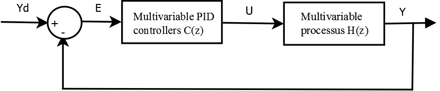
Figure 1: A multivariable PID control system.

Three kinds of performance criteria usually considered in the control design are integral of the Absolute Error (IAE), integral of Square Error (ISE) and integral of Time weighted Square Error (ITSE) which are given as:

$$\textbf{IAE}=|{e_{1}(k)+e_{2}(k)}+...+e_{n}(k)|$$ (15)

$$\textbf{ISE}=\sum{e_{1}(k)}^{2}+\sum{e_{2}(k)}^{2}+...+\sum{e_{n}(k)}^{2}$$ (16)

$$\textbf{ITSE}=\sum k*{e_{1}(k)}^{2}+\sum k*{e_{2}(k)}^{2}+...+\sum k*{e_{n}(k)}^{2}$$ (17)

Therefore, for the PSO-based PID tuning, these performance indexes (Eqs. (17)-(19)) will be used as the objective function. In other word, the objective in the PSO-based optimization is to seek a set of PID parameters such that the feedback control system has minimum performance index.

IV-A Tuning of PID uzing Z-N method

The first method of Z-N tuning is based on the open-loop step response of the system. The open-loop system s Shaped response is characterized by the parameters, namely the process time constant $T$ and $L$. These parameters are used to determine the controller s tuning parameters (see TABLE.1).

TABLE I: Ziegler-Nichols open-loop tuning parameter

Controller	kp	Ti=kp/ki	Td=kd/kp
P	T/L	-	0
PI	0.9(T/L)	L/0.3	0
PID	1.2(T/L)	2L	0.5L

The second method of Z-N tuning is closed-loop tuning method that requires the determination of the ultimate gain and ultimate period. The method can be interpreted as a technique of positioning one point on the Nyquist curve [13]. This can be achieved by adjusting the controller gain (Ku) till the system undergoes sustained oscillations (at the ultimate gain or critical gain), whilst maintaining the integral time constant ( Ti ) at infinity and the derivative time constant (Td) at zero (see TABLE.2).

TABLE II: Ziegler-Nichols closed-loop tuning parameter

Controller	kp	Ti=kp/ki	Td=kd/kp
P	0.5ku	-	0
PI	0.45ki	1.5kp/Pu	0
PID	0.6ku	2kp/Pu	kpPu/8

IV-B Implementation of PSO-Based PID Tuning

IV-B1 Particle swarm optimization (PSO)

Particle swarm optimization was introduced by Kennedy and Eberhart by simulating social behavior of birds flocks in (199[10]. The PSO algorithm has been successfully applied to solve various optimization problems [14]. The PSO works by having a group of m particles. Each particle can be considered as a candidate solution to an optimization problem and it can be represented by a point or a position vector $\textbf{X}_{ij}=[X_{i1},...,X_{id}]$ in a d dimensional search space which keeps on moving toward new points in the search space with the addition of a velocity vector $\textbf{V}_{ij}=[V_{i1},...,V_{id}]$ to further facilitate the search procedure. The initial positions and velocities of particles are random from a normal population in the interval [0, 1]. All particles move in the search space to optimize an objective function f. Each member of the group gets a score after evaluation on objective function f. The score is regarded as a fitness value. The member with the highest score is called global best. Each particle memorizes its previous best positions. During the search process all particles move toward the areas of potential solutions by utilizing the cognitive and social learning components. The process is repeated until any prescribed stopping criterion is reached. After any iteration, all particles update their positions and velocities to achieve better fitness values according to the following:

$$\textbf{V}_{pd}^{t+1} = \omega\textbf{V}_{pd}^{t}+c_{1}r_{1}(\textbf{pbest}^{t}-\textbf{X}_{pd}^{t})$$

$$+ c_{2}r_{2}(\textbf{gbest}^{t}-\textbf{X}_{id}^{k}),$$

$$\textbf{X}_{pd}^{t+1} = \textbf{X}_{pd}^{t}+\textbf{V}_{pd}^{t+1},$$ (19)

where:
$t$ is the current iteration number, $\textbf{pbest}_{i}$ is ${pbest}$ of particle $i$, $\textbf{gbest}_{g}$ is ${gbest}$ of the group, $r_{1},r_{2}$ are two random numbers in the interval [0, 1], $c_{1},c_{2}$ are positive constants and $w$ is the inertia weight,is a parameter used to control the impact of the previous velocities on the current velocity. It influences the tradeoff between the global and local exploitation abilities of the particles. Weight is updated as:

$$\omega=\omega_{\max}-\left({\frac{{\omega\max-\omega_{\min}}}{{iter_{\max}}}}\right)iter$$ (20)

where $\omega_{\min}$, $\omega_{\max}$, $iter$, and $iter_{\max}$ are minimum, maximum values of $\omega$ , the current iteration number and pre-specified maximum number of iteration cycles, respectively.

IV-B2 Proposed PSO-PID Controller

This paper presents a PSO-PID controller for searching the optimal controllers parameters of MIMO nonlinear system ,$kp_{i}$ , $ki_{i}$ and , $kd_{i}$ with the PSO algorithm. Each individual $K_{i}$ contains 3*m members $kp_{i}$ , $ki_{i}$ and , $kd_{i}$. Its dimension is n*3*m. The searching procedures of the proposed PSO-PID controller were shown as below [12]. Optimal design for both conventional PID controllers can be fulfilled using PSO technique. Based on the PSO technique, the PID controller can be tuned to some parameters values that minimize those fitness functions given in (15), (16) and(17). The algorithmic steps for the PSO is as follows:

• Step 1: Select the number of particles, generations, tuning accelerating coefficients $c_{1}$ and $c_{2}$ and random numbers $r_{1}$, and $r_{2}$ to start the optimal solution searching.

• Step 2: Initialize the particle position and velocity.

• Step 3: Select the particle s individual best value for each generation.

• Step 4: Select the particle s global best value, particle near the target among all the particles, is obtained by comparing all the individual best values.

• Step 5: Update particle individual best pbest , global best gbest , in the velocity equation (18) and obtain the new velocity.

• Step 6: Update the new velocity value in Eq. (19) and obtain the position of the particle.

• Step 7: Find the optimal solution with a minimum (IAE, ISE, ITSE) from the updated new velocity and position values.

V SIMULATION RESULTS

This section presents a simulation example to shown an application of the proposed control algorithm and its satisfactory performance. The MIMO nonlinear system is characterized by the equation(16), [16][17].

$$\left\{\begin{array}[]{ll}y1(k)=\frac{a_{1}y_{1}(k-1)y_{2}(k-1)}{1+a_{2}y_{1}^{2}(k-1)+a_{3}y_{2}^{2}(k-1)}+\\ \,\,\,\,\,\,\,a_{4}u_{1}(k-2)+a_{5}u_{1}(k-1)+a_{6}u_{2}(k-1)\\ y_{2}(k)=\frac{b_{1}y_{2}(k-1)sin(y_{2}(k-2))}{1+b_{2}y_{2}^{2}(k-1)+b_{3}y_{1}^{2}(k-1)}+\\ \,\,\,\,\,\,\,b_{4}u_{2}(k-2)+b_{5}u_{2}(k-1)+b_{6}u_{1}(k-1)\end{array}\right.$$ (21)

The system parameters are: $a_{1}=0.7,a_{2}=1,a_{3}=1,a_{4}=0.3,a_{5}=1,a_{6}=0.2,b_{1}=0.5,b_{2}=1,b_{3}=1,b_{4}=0.5,b_{5}=1andb_{6}=0.2$ which is used as a test for control techniques introduced in this paper, to demonstrate the effectiveness of the proposed algorithms. Here $y_{1}$ and $y_{2}$ are the outputs, $u_{1}$ and $u_{2}$ are the inputs which is uniformly bounded in the region $[-2,2]$.
We choose $[y_{1}(k-1),y_{1}(k-2),u_{1}(k-1),u_{1}(k-2),u_{2}(k-1)]$ and $[y_{2}(k-1),y_{2}(k-2),u_{2}(k-1),u_{2}(k-2),,u_{2}(k-1)]$ as inputs variables, and the number of fuzzy rules is four. The setup applied in this work was the following: the population size was 20, the stopping criterion was 30 generations, $\omega_{min}=0.5$, $\omega_{max}=0.9$, and $c_{1}=c_{2}=2$.

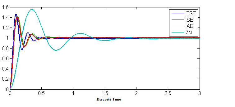
Figure 2: System response (y1)

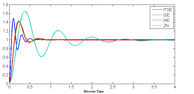
Figure 3: System response (y2)

TABLE III: Optimized PID parameters (y1)

Tuning Method	kp	ki	kd
Z-N-PID	32.3431	3.2943	4.4829
PSO-PID1 (ISE)	$26.7236$	46.2192	30.136
PSO-PID1 (IAE)	$8.7263$	46.2192	33.1360
PSO-PID1 (ITSE)	$5.3487$	15.7988	45.4369

TABLE IV: Optimized PID parameters (y2)

Tuning Method	kp	ki	kd
Z-N PID	38.0743	4.6739	5.6734
PSO-PID1 (ISE)	$35.7236$	16.2192	9.136
PSO-PID2 (IAE)	$39.5246$	17.2514	9.7983
PSO-PID3 (ITSE)	$45.3487$	15.7988	41.4369

TABLE V: Step response performance for PID controllers (y1)

Tuning Method	Overshoot(%)	Rise Time	Setting Time
Z-N PID	55.3483	0.1264	1.6733
SPSO-PID1 (ISE)	$41.6977$	0.0474	0.6182
PSO-PID2 (IAE)	$40.5825$	0.0453	0.4791
PSO-PID3 (ITSE)t	$46.1849$	0.0374	0.4246

TABLE VI: Step response performance for PID controllers (y2)

Tuning Method	Overshoot(%)	Rise Time	Setting Time
Z-N PID	64.8174	0.1352	3.2941
PSO-PID1 (ISE)	$40.8062$	0.0929	0.7970
PSO-PID2 (IAE)	$42.3434$	0.0884	0.7775
PSO-PID3 (ITSE)	$48.5050$	0.0389	0.5265

In the conventionally Z-N tuned PID controller, the systems response produces high overshoot, but a better performance obtained with the implementation of PSO-based PID controller tuning. In the PSO-based PID controllers (PSO-PID), different performance index gives different results. These are shown in TABLE. III and TABLE. IV. Comparative results for the PID controllers are given below in TABLE. V and TABLE. VI where the step response performance is evaluated based on the overshoot, settling time and Rise time. The corresponding plot for the step responses are shown in Fig. 2 and Fig.3.

VI CONCLUSIONS

This paper presents a design method for determining the PID controller parameters using the PSO method for MIMO nonlinear systems. The proposed method integrates the PSO algorithm with performance criterions into a PSO-PID controller. The comparison between PSO-based PID (PSO-PID) performance and the ZN-PID is presented. The results show the advantage of the PID tuning using PSO-based optimization approach.

References

- [1] Astrom. K. J and H gglund. T, PID Controllers: Theory, Design, and Tuning, ISBN-10: 1556175167, ISBN-13. 978-1556175169, Edition. 2 Sub, January 1, 1995.
- [2] N. Suda, PID Control, Asakura Publishing company, Ltd., ISBN 978-4-254-20966-2, Tokyo, 1992.
- [3] Luyben. W. L. , A simple method for tuning SISO controllers in a multivariable system, Industrial Engineering Chemistry Product Research and Development, vol. 25, pp. 654 660, 1986.
- [4] Yusof, R., Omatu, S. , A multivariable self-tuning PID controller, Internal Journal of Control, vol. 57(6), pp. 1387 1403, 1993.
- [5] Wang. Q. G, Zou. B, Lee. T. H, Qiang. B, Auto-tuning of multivariable PID controllers from decentralized relay feedback, Automatica, vol. 33(3), pp. 319 330, 1997.
- [6] Kennedy. J, and Eberhart. C, Particle Swarm Optimization, Proceedings of the IEEE International Conference on Neural Networks, Australia, pp. 1942-1948, 1995.
- [7] Oliveira. P. M, Cunha. J. B, and Coelho. J. o,Design of PID controllers using the Particle Swarm Algorithm, Twenty-First IASTED International Conference: Modeling, Identification, and Control, Innsbruck, Austria, 2002.
- [8] Lagrat. I, Ouakka. H and Boumhidi. L. I, Fuzzy clustring for identification of Takagi-Sugeno fuzzy models of a class of nonlinear multivariable systems, Facult Des Sciences, B. P, Atlas, 30000 Fez- MOROCCO, 1996.
- [9] Takagi. T, Sugeno. M, Fuzzy Identification of Systems and its Application to Modeling and Control, IEEE Transactions on Systems, Man and Cybernetics, vol. 15(1), pp. 116-132, 1985.
- [10] Qin. S. J and Badgwell. T. A, A survey of industrial model predictive control technology, Control Engineering Practice, vol. 11, pp. 733-764, 2003.
- [11] Chang. W. D, A multi-crossover genetic approach to multivariable PID controllers tuning, Department of Computer and Communication, Shu-Te University, Kaohsiung 824, Taiwan, Expert Systems with Applications, vol. 33 pp. 620-626, 2007.
- [12] Morkos. S, Kamal. H, Optimal Tuning of PID Controller using Adaptive Hybrid Particle Swarm Optimization Algorithm, Int. J. of Computers, Communications and Control, ISSN pp. 1841-9836, 2012.
- [13] Astrom. K. J. and Hagglund. t, PID Controllers: Theory, Design and Tuning, ISA, Research Triangle, Par, NC, 1995.
- [14] Soltani, M., Chaari, A. and Benhmida, F. , A novel fuzzy c regression model algorithm using new measure of error and based on particle swarm optimization, International Journal of Applied Mathematics and Computer Science, Vol. 22, No. 3, pp. 617-628, 2012.
- [15] I. Lagrat. I, Ouakka. H and Boumhidi. I, Fuzzy adaptive control of a class of MISO nonlinear systems, Control and Cybernetics, vol. 37, No. 1, 2008.
- [16] Song. F and Li. P, MIMO Decoupling Control Based on Support Vector Machines -order Inversion. Proceedings of the 6th World Congress on Intelligent Control and Automation, Dalian-China, pp. 1002-1006, 2006.
- [17] Petlenkov. E, NN-ANARX Structure Based Dynamic Output Feedback Linearization for Contro of Nonlinear MIMO Systems, Proceedings of the 15th Mediterranean Conference on Control and Automation, Athens-Greece, pp. 1-6, 2007.