Magnetohydrodynamic stability of stochastically driven accretion flows

Abstract

We investigate the evolution of magnetohydrodynamic/hydromagnetic perturbations in the presence of stochastic noise in rotating shear flows. The particular emphasis is the flows whose angular velocity decreases but specific angular momentum increases with increasing radial coordinate. Such flows, however, are Rayleigh stable, but must be turbulent in order to explain astrophysical observed data and, hence, reveal a mismatch between the linear theory and observations/experiments. The mismatch seems to have been resolved, atleast in certain regimes, in the presence of weak magnetic field revealing magnetorotational instability. The present work explores the effects of stochastic noise on such magnetohydrodynamic flows, in order to resolve the above mismatch generically for the hot flows. We essentially concentrate on a small section of such a flow which is nothing but a plane shear flow supplemented by the Coriolis effect, mimicking a small section of an astrophysical accretion disk around a compact object. It is found that such stochastically driven flows exhibit large temporal and spatial auto-correlations and cross-correlations of perturbation and hence large energy dissipations of perturbation, which generate instability. Interestingly, auto-correlations and cross-correlations appear independent of background angular velocity profiles, which are Rayleigh stable, indicating their universality. This work, to the best of our knowledge, is the first attempt to understand the evolution of three-dimensional hydromagnetic perturbations in rotating shear flows in the presence of stochastic noise.

I Introduction

Recently, Mukhopadhyay & Chattopadhyay mc13 (see, the references therein) have initiated exploring effects of stochastic noise in rotating shear flows in three dimensions with particular emphasize to astrophysical accretion disks. They have essentially addressed the evolutions of pure hydrodynamic perturbations and found them to be adequate enough to explain instability and subsequent turbulence therein. This is in accordance with the fact that in three dimensions, one requires to invoke extra physics to reveal large energy growth or even instability in the system bmraha . This is very important for charge natural flows like accretion disks around quiescent cataclysmic variables, in protoplanetary and star-forming disks, and the outer region of disks in active galactic nuclei etc. where flows are cold and of low ionization and effectively neutral in charge.

In the cases of hot flows, e.g. disks around black holes, magnetorotational instability is generally believed to be responsible for turbulence and hence transport of angular momentum therein. The problem has been well studied and has had a long history of fluid mechanical insight into the rotating shear flows and subsequently accretion disk problem in the linearly stable regime, when origin of turbulence is a major issue gu ; kim ; mk ; man ; rud ; dau ; zahn ; klar ; dub1 ; dub2 . Based on ‘shearing sheet’ approximation, without balbusetal96 ; hawleyetal99 and with ll05 explicit viscosity, some authors attempted to tackle the issue of turbulence in hot accretion disks. However, other authors argued for limitations in this work pumir96 ; fromang-papaloizou07 . While the authors, who did not include explicit viscosity, could not directly define a Reynolds number ($R_{e}$), their estimated $R_{e}$ from the simulations is $\sim 10^{3}-10^{4}$. They also did not find any evidence for a subcritical transition to turbulence. Based on the simulations including explicit viscosity, other authors could achieve $R_{e}\approx 4\times 10^{4}$, and concluded that Keplerian like flows could exhibit very weak turbulence, particularly in absence of magnetic field. However, the recent experimental results by Paoletti et al. paoletti , clearly argue for the significant level of transport from hydrodynamics alone. Moreover, the results from direct numerical simulations avila also argue for hydrodynamic instability and turbulence at low $R_{e}$.

In the present paper, we extend the work by Mukhopadhyay & Chattopadhyay mc13 and investigate the amplification of linear magnetohydrodynamic/hydromagnetic perturbations in Rayleigh stable rotating, hot, shear flows in the presence of stochastic noise in three dimensions, leading to instability and plausible turbulence. The earlier paper mc13 already summarized the association of growing, unstable modes generated by perturbed flows with statistical physics, in particular effects of noise in such flows, based on which the present work has been founded. Hence we do not repeat them here. The effects of white noise in a linear, nonrotating, non-magnetized shear flow, which is non-normal in nature, was also studied by earlier authors ep03 . In the present study, we implement the ideas of statistical physics, already implemented by above authors, to rotating, magnetized, shear flows in order to obtain the correlation energy growths of fluctuation/perturbation and underlying scaling properties.

In the next section, we first recall the equations describing the stochastically forced perturbed flows, namely magnetized version of the set of Orr-Sommerfeld and Squire equations proposed by Mukhopadhyay & Chattopadhyay mc13 in the presence of noise, which are to be solved for the present purpose. Subsequently, in §3 we investigate the temporal and spatial auto-correlations and cross-correlations of perturbation in the presence of white noise in detail, in order to understand the plausible instability in the flows. In §4, we study the correlations in the presence of colored noise. Finally, we summarize the results with conclusions in §5.

II Equations describing perturbed magnetized rotating shear flows in the presence of noise

The linearized Navier-Stokes equation in the presence of background plane shear $(0,-x,0)$ and magnetic field $(0,B_{1},1)$, when $B_{1}$ being a constant, both expressed in the dimensionless units, in the presence of background angular velocity profile $\Omega\propto r^{-q}$, when $r$ being the distance from the center of the system, in a small section of the incompressible flow with $-l/2\leq x\leq l/2$, has already been established mc13 . The underlying equations are nothing but the linearized set of hydromagnetic equations including the equations of induction in a local Cartesian coordinate. Here, we plan to work with the dimensionless variables, when any length is expressed in units of the size of system $L$ in the $x-$direction, the time in units of the inverse of background angular velocity of the flow about $z-$direction $\Omega$, the velocity in $q\Omega L$ ($1\leq q<2$), and other variables are expressed accordingly (see, e.g., man ; bmraha ; mc13 for detailed description of the choice of coordinate in a small section). Hence, in dimensionless units, the set of equations is given by

$$\left(\frac{\partial}{\partial t}-x\frac{\partial}{\partial y}\right)u-\frac{2v}{q}+\frac{\partial p_{\rm tot}}{\partial x}-\frac{1}{4\pi}\left(B_{1}\frac{\partial B_{x}}{\partial y}+\frac{\partial B_{x}}{\partial z}\right)=\frac{1}{R_{e}}\nabla^{2}u,$$ (1)

$$\left(\frac{\partial}{\partial t}-x\frac{\partial}{\partial y}\right)v+\left(\frac{2}{q}-1\right)u+\frac{\partial p_{\rm tot}}{\partial y}-\frac{1}{4\pi}\left(B_{1}\frac{\partial B_{y}}{\partial y}+\frac{\partial B_{y}}{\partial z}\right)=\frac{1}{R_{e}}\nabla^{2}v,$$ (2)

$$\left(\frac{\partial}{\partial t}-x\frac{\partial}{\partial y}\right)w+\frac{\partial p_{\rm tot}}{\partial z}-\frac{1}{4\pi}\left(B_{1}\frac{\partial B_{z}}{\partial y}+\frac{\partial B_{z}}{\partial z}\right)=\frac{1}{R_{e}}\nabla^{2}w,$$ (3)

$$\frac{\partial B_{x}}{\partial t}=\frac{\partial u}{\partial z}+B_{1}\frac{\partial u}{\partial y}+x\frac{\partial B_{x}}{\partial y}+\frac{1}{R_{m}}\nabla^{2}B_{x},$$ (4)

$$\frac{\partial B_{y}}{\partial t}=\frac{\partial v}{\partial z}+B_{1}\frac{\partial v}{\partial y}-x\frac{\partial B_{x}}{\partial x}-x\frac{\partial B_{z}}{\partial z}-B_{x}+\frac{1}{R_{m}}\nabla^{2}B_{y},$$ (5)

$$\frac{\partial B_{z}}{\partial t}=\frac{\partial w}{\partial z}+B_{1}\frac{\partial w}{\partial y}+x\frac{\partial B_{z}}{\partial y}+\frac{1}{R_{m}}\nabla^{2}B_{z},$$ (6)

when the vectors for velocity and magnetic field perturbations are $(u,v,w)$ and $(B_{x},B_{y},B_{z})$ respectively, $R_{e}$ and $R_{m}$ are the hydrodynamic and magnetic Reynolds numbers respectively, $p_{\rm tot}$ is the total pressure perturbation (including that due to the magnetic field). Above equations are supplemented by the conditions for incompressibility and absence of magnetic charge, given respectively by

$$\frac{\partial u}{\partial x}+\frac{\partial v}{\partial y}+\frac{\partial w}{\partial z}=0,$$ (7)

$$\frac{\partial B_{x}}{\partial x}+\frac{\partial B_{y}}{\partial y}+\frac{\partial B_{z}}{\partial z}=0.$$ (8)

Now the above equations in the presence of stochastic noise can be recasted into magnetized version of Orr-Sommerfeld and Squire equations in the presence of the Coriolis force, given by mc13

$$\left(\frac{\partial}{\partial t}-x\frac{\partial}{\partial y}\right)\nabla^{2}u+\frac{2}{q}\frac{\partial\zeta}{\partial z}-\frac{1}{4\pi}\left(B_{1}\frac{\partial}{\partial y}+\frac{\partial}{\partial z}\right)\nabla^{2}B_{x}=\frac{1}{R_{e}}\nabla^{4}u+\eta_{1}(x,t),$$ (9)

$$\left(\frac{\partial}{\partial t}-x\frac{\partial}{\partial y}\right)\zeta+\frac{\partial u}{\partial z}-\frac{2}{q}\frac{\partial u}{\partial z}-\frac{1}{4\pi}\left(B_{1}\frac{\partial}{\partial y}+\frac{\partial}{\partial z}\right)\zeta_{B}=\frac{1}{R_{e}}\nabla^{2}\zeta+\eta_{2}(x,t),$$ (10)

$$\left(\frac{\partial}{\partial t}-x\frac{\partial}{\partial y}\right)B_{x}-B_{1}\frac{\partial u}{\partial y}-\frac{\partial u}{\partial z}=\frac{1}{R_{m}}\nabla^{2}B_{x}+\eta_{3}(x,t),$$ (11)

$$\left(\frac{\partial}{\partial t}-x\frac{\partial}{\partial y}\right)\zeta_{B}-\frac{\partial\zeta}{\partial z}-B_{1}\frac{\partial\zeta}{\partial y}-\frac{\partial B_{x}}{\partial z}=\frac{1}{R_{m}}\nabla^{2}\zeta_{B}+\eta_{4}(x,t).$$ (12)

where $\eta_{1,2,3,4}$ are the components of noise arising in the linearized system due to stochastic perturbation such that $<\eta_{i}(\vec{x},t)\eta_{j}(\vec{x}^{\prime},t^{\prime})>=D_{i}(\vec{x})\>\delta^{3}(\vec{x}-\vec{x}^{\prime})\>\delta(t-t^{\prime})\>\delta_{ij}$. The long time, large distance behaviors of the correlations of noise are encapsulated in $D_{i}(\vec{x})$ which is a structure pioneered by Forster, Nelson & Stephen nelson . In the Fourier space, however, the structure of the correlation function $D_{i}(\vec{k})$ depends on the regime under consideration. It can be shown for all (non-linear) non-inertial flows nelson ; akc_shear that $D_{i}(k)\sim 1/k^{d}$, where $d$ is the spatial dimension, without vertex correction and $D_{i}(k)\sim 1/k^{d-\alpha}$, with $\alpha>0$, in the presence of vertex correction. Note, however, that $D_{i}(\vec{x})$ is constant for white noise.

As before mc13 we focus onto the narrow gap limit, where in a local analysis we consider a small radially confined region of the flow, while the azimuthal and vertical confinements are imposed by a periodic boundary conditions accordingly in such a way that the perturbation wave-vector can be assumed to be isotropic. Note that it could be easily extended to a free-slip case. The only modification this would bring about is in the values of the limits (now finite, instead of infinite). Apart from complicating the calculation of the resultant integrals which will have poles of different nature in different ranges of $k$, this would not serve in bringing any practical change for the present purpose. For further details, see Mukhopadhyay & Chattopadhyay mc13 . Hence, we can resort to a Fourier series expansion of $u$, $\zeta$, $B_{x}$, $\zeta_{B}$ and $\eta_{i}$ as

$$u(\vec{x},t)=\int\tilde{u}_{\vec{k},\omega}\,e^{i(\vec{k}.\vec{x}-\omega t)}d^{3}k\,d\omega,$$

$$\zeta(\vec{x},t)=\int\tilde{\zeta}_{\vec{k},\omega}\,e^{i(\vec{k}.\vec{x}-\omega t)}d^{3}k\,d\omega,$$

$$B_{x}(\vec{x},t)=\int\tilde{B_{x}}_{\vec{k},\omega}\,e^{i(\vec{k}.\vec{x}-\omega t)}d^{3}k\,d\omega,$$

$$\zeta_{B}(\vec{x},t)=\int\tilde{\zeta_{B}}_{\vec{k},\omega}\,e^{i(\vec{k}.\vec{x}-\omega t)}d^{3}k\,d\omega,$$

$$\eta_{i}(\vec{x},t)=\int\tilde{\eta_{i}}_{\vec{k},\omega}\,e^{i(\vec{k}.\vec{x}-\omega t)}d^{3}k\,d\omega,$$ (13)

and substituting them into equations (9), (10), (11) and (12) we obtain

$$\left(\begin{array}[]{cr}\tilde{u}_{\vec{k},\omega}\\ \tilde{\zeta}_{\vec{k},\omega}\\ \tilde{B}_{x_{\vec{k},\omega}}\\ \tilde{\zeta_{B}}_{\vec{k},\omega}\end{array}\right)={\cal M}^{-1}\left(\begin{array}[]{cr}\tilde{\eta_{1}}_{\vec{k},\omega}\\ \tilde{\eta_{2}}_{\vec{k},\omega}\\ \tilde{\eta_{3}}_{\vec{k},\omega}\\ \tilde{\eta_{4}}_{\vec{k},\omega}\end{array}\right),$$ (22)

where

$${\cal M}=\left(\begin{array}[]{cr}{\cal M}_{11}\,\,\,\,\,{\cal M}_{12}\,\,\,\,\,{\cal M}_{13}\,\,\,\,\,{\cal M}_{14}\\ {\cal M}_{21}\,\,\,\,\,{\cal M}_{22}\,\,\,\,\,{\cal M}_{23}\,\,\,\,\,{\cal M}_{24}\\ {\cal M}_{31}\,\,\,\,\,{\cal M}_{32}\,\,\,\,\,{\cal M}_{33}\,\,\,\,\,{\cal M}_{34}\\ {\cal M}_{41}\,\,\,\,\,{\cal M}_{42}\,\,\,\,\,{\cal M}_{43}\,\,\,\,\,{\cal M}_{44}\end{array}\right),$$ (27)

$${\cal M}_{11}=ik^{2}\omega+ilk^{2}k_{y}-\frac{k^{4}}{R_{e}},\hskip 5.69054pt{\cal M}_{12}=\frac{2ik_{z}}{q},\hskip 5.69054pt{\cal M}_{13}=\frac{ik^{2}}{4\pi}(B_{1}k_{y}+k_{z}),\hskip 5.69054pt{\cal M}_{14}=0,$$

$${\cal M}_{21}=ik_{z}\left(1-\frac{2}{q}\right),\hskip 5.69054pt{\cal M}_{22}=-i\omega-ilk_{y}+\frac{k^{2}}{R_{e}},\hskip 5.69054pt{\cal M}_{23}=0,\hskip 5.69054pt{\cal M}_{24}=\frac{-i}{4\pi}\left(B_{1}k_{y}+k_{z}\right),$$

$${\cal M}_{31}=\left(-iB_{1}k_{y}-ik_{z}\right),\hskip 5.69054pt{\cal M}_{32}=0,\hskip 5.69054pt{\cal M}_{33}=\left(-i\omega-ilk_{y}+\frac{k^{2}}{R_{m}}\right),\hskip 5.69054pt{\cal M}_{34}=0,$$

$${\cal M}_{41}=0,\hskip 5.69054pt{\cal M}_{42}=\left(-iB_{1}k_{y}-ik_{z}\right),\hskip 5.69054pt{\cal M}_{43}=-ik_{z},\hskip 5.69054pt{\cal M}_{44}=\left(-i\omega-ilk_{y}+\frac{k^{2}}{R_{m}}\right),$$ (28)

when $\tilde{{\eta}_{i}}_{\vec{k},\omega}$; $i=1,2,3,4$, are the components of noise in $k-\omega$ space, $k=\sqrt{k_{x}^{2}+k_{y}^{2}+k_{z}^{2}}$. See mc13 for other details.

III Two-point correlations of perturbation in the presence of white noise

We now look at the spatio-temporal auto-correlations and cross-correlations of the perturbation flow fields $u$, $\zeta$, $B_{x}$ and $\zeta_{B}$ for very large $R_{e}$ and $R_{m}$ barabasi_stanley . This choice of large $R_{e}/R_{M}$ is quite meaningful for astrophysical flows. For the present purpose, the magnitudes and gradients (scalings) of these correlations of perturbations would plausibly indicate noise induced instability which could lead to turbulence in rotating shear flows.

III.1 Temporal correlation

III.1.1 Auto-correlations

Assuming $<\tilde{\eta_{i}}_{\vec{k},\omega}\,\tilde{\eta_{j}}_{-\vec{k},-\omega}>=\delta_{ij}$, without loss of any important physics, we obtain the temporal correlations of velocity, vorticity, magnetic field and magnetic vorticity perturbations given below as

$$<u(\vec{x},t)\,u(\vec{x},t+\tau)>=C_{u}(\tau)=\int d^{3}k\,d\omega\,e^{-i\omega\tau}<\tilde{u}_{\vec{k},\omega}\,\tilde{u}_{-\vec{k},-\omega}>$$

$$<\zeta(\vec{x},t)\,\zeta(\vec{x},t+\tau)>=C_{\zeta}(\tau)=\int d^{3}k\,d\omega\,e^{-i\omega\tau}<\tilde{\zeta}_{\vec{k},\omega}\,\tilde{\zeta}_{-\vec{k},-\omega}>$$

$${\hskip-36.98866pt<B_{x}(\vec{x},t)\,\ B_{x}(\vec{x},t+\tau)}>=C_{B_{x}}(\tau)=\int d^{3}k\,d\omega\,e^{-i\omega\tau}<\tilde{B_{x}}_{\vec{k},\omega}\,\tilde{B_{x}}_{-\vec{k},-\omega}>$$

$${\hskip-36.98866pt<\zeta_{B}(\vec{x},t)\,\,\zeta_{B}(\vec{x},t+\tau)}>=C_{\zeta_{B}}(\tau)=\int d^{3}k\,d\omega\,e^{-i\omega\tau}<\tilde{\zeta_{B}}_{\vec{k},\omega}\,\tilde{\zeta_{B}}_{-\vec{k},-\omega}>.$$ (29)

We further consider the projected hyper-surface for which $k_{x}=k_{y}=k_{z}=k/\sqrt{3}$, without much loss of generality for the present purpose. This corresponds to a special choice of initial perturbation. As our one of the major interests is to understand the scaling laws, this restriction would not matter, which however may affect the magnitude of the correlations. This further helps in introducing the incompressibility constraints on the noise in the corresponding representation easily, which becomes independent of $k$ (see ep03 for details).

We now perform the $\omega$-integration of the integrands in equation (29) by computing the four second order poles of the kernel which are functions of $k$. The form of all the integrands in equation (29) is given by

$$f(k,\omega)=\frac{p(k,\omega)}{[\omega-\omega_{1}(k)]^{2}[\omega-\omega_{2}(k)]^{2}[\omega-\omega_{3}(k)]^{2}[\omega-\omega_{4}(k)]^{2}},$$

which clearly reveals second order poles at $\omega_{1},\omega_{2},\omega_{3}$ and $\omega_{4}$. We choose the range of $k$ in such a way that the poles lie in the upper-half of the complex plane. Then by summing up the residues at the appropriate poles, we evaluate the magnitude of frequency part of the integration. Finally, integrating the rest from $k_{0}$ to $k_{m}$, where $k_{0}=2\pi/l_{\rm max}$, $k_{m}=2\pi/l_{\rm min}$ and $l=l_{\rm max}-l_{\rm min}$, being the size of the chosen small section of the flow in the radial direction (chosen to be $2$ throughout for the present calculations), we obtain $C_{u}(\tau)$, $C_{\zeta}(\tau)$, $C_{B_{x}}(\tau)$ and $C_{\zeta_{B}}(\tau)$.

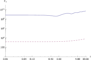
Figure 1: Comparing temporal auto-correlations of velocity, when $q=1.5$, between magnetic (solid line) and non-magnetic (dashed line) flows.

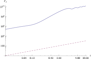
Figure 2: Comparing temporal auto-correlations of velocity, when flows are nonrotating, between magnetic (solid line) and non-magnetic (dashed line) flows.

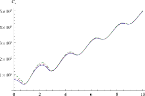
Figure 3: Temporal auto-correlations of velocity, when $q=1.5$ (solid line), $1.7$ (dashed line), $1.9$ (dotted line), $1.9999$ (dotdashed line).

First of all, we show in Figures 1 and 2 that independent of the effects due to rotation and noise, the presence of magnetic field solely increases the auto-correlation enormously compared to that in the absence of magnetic field. This establishes the power of magnetic field and associated Alfvén wave in modulating the growth of perturbation. This further establishes the importance of the present work over that by Mukhopadhyay & Chattopadhyay mc13 .

Now we concentrate on magnetized flows. Figure 3 shows that in the magnetic flows with the decrease of $q$, although the velocity correlation decreases, the difference between those of any two $q$s is insignificant. Hence, the simultaneous presence of magnetic field and stochastic white noise kills the dependence of correlations on the rotational effect.

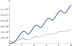
Figure 4: Same as Figure 1, but auto-correlation for nonrotating flow (thick-solid line) is additionally shown.

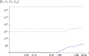
Figure 5: Temporal auto-correlations of velocity (solid line), vorticity (dashed line), magnetic field (dotted line) and magnetic vorticity (dot-dashed line), when $q=1.5$.

Note that in the absence of noise, hydrodynamic perturbation energy growth (and hence $C_{u}(\tau)$) in all the above rotating cases, essentially for $q<2$, is very small, as shown previously man , particularly in three dimensions. However, the effects of magnetic field and noise bring in a huge growth of the perturbation top of the Coriolis fluctuations, clearly revealing instability. A remarkable feature in the scaling nature of all these correlations is their independence of $q$ (background angular velocity profile) — a trait identified in statistical physics literature as universality.

In Figure 4, we show that the correlation for a nonrotating magnetized flow appears to be quite larger compared to that for rotating flows, which is similar to the trait observed in the absence of noise (see, e.g., bmraha ; man ). However, the presence of noise increases the growth of perturbations enormously in either of the cases.

Figure 5 depicts that the auto-correlation for vorticity perturbation is largest among all the auto-correlations for a particular $q$. Note also that auto-correlations for velocity and magnetic vorticity exhibit more oscillations compared to that for magnetic field and vorticity. This is because the effects due to Alfvén wave arised from magnetic field. Note from equations (9) and (12) that the evolutions of velocity and magnetic vorticity depend on the magnetic perturbation explicitly, and hence the respective auto-correlations get modulated by Alfvén waves. Moreover, the amplitude of velocity correlation is smallest at the beginning due to fluctuations arised in the velocity perturbation, whose curl however need not be small, giving rise to large vorticity correlations. However, either of correlations is large enough to govern instability and then turbulence. Nevertheless, all the correlations saturate (or tend to saturate) at a relatively large $\tau$ (which is more clearer in the log-linear plots described in §V).

III.1.2 Cross-Correlations

Here we stick to the same assumptions as of the computations of auto-correlations. The temporal cross-correlation of two quantities, e.g. $u$ and $\zeta$, is defined by

$$<u(\vec{x},t)\,\zeta(\vec{x},t+\tau)>=C_{u\zeta}(\tau)=\int d^{3}k\,d\omega\,e^{-i\omega\tau}<\tilde{u}_{\vec{k},\omega}\,\tilde{\zeta}_{-\vec{k},-\omega}>.$$ (30)

Similarly, one can define other cross-correlations. We solve the integrals following the same procedure as described for auto-correlations.

First of all, we show in Figure 6 that unlike auto-correlations, the cross-correlation of velocity and vorticity decreases quite a bit in the presence of magnetic field compared to that in the absence of it at the beginning. This further pinpoints the additional effects arised due to the magnetic field.

Figure 7 shows all the cross-correlations in a magnetized Keplerian disk. Interestingly, cross-correlations of velocity and magnetic vorticity (dashed line) and vorticity and magnetic field (dotted line) have a steady, constant, higher amplitude at the beginning compared to other cross-correlations. This is because they are correlations of either two fluctuating (due to Alfvén wave) variables or two non-fluctuating variables, when, as shown in Figure 5 that, one of them have larger amplitude to begin with. All the remaining ones are the correlations of a strongly Alfvén wave modulated variable with a non-modulated variable. Because of the same reason, the velocity-vorticity cross-correlation in the non-magnetized flow is larger than that in the magnetized flow, when magnetic field modulates velocity perturbation but not the vorticity perturbation.

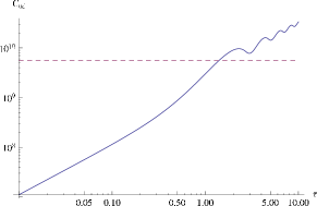
Figure 6: Comparing temporal cross-correlations of velocity and vorticity, when $q=1.5$, between magnetic (solid line) and non-magnetic (dashed line) flows.

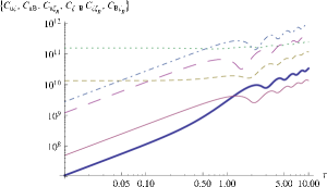
Figure 7: Temporal cross-correlations of velocity and vorticity (thick solid line), velocity and magnetic field (solid line), velocity and magnetic vorticity (dashed line), vorticity and magnetic field (dotted line), vorticity and magnetic vorticity (dot-dashed line), magnetic field and magnetic vorticity (long dashed line), when $q=1.5$.

III.2 Spatial correlation

III.2.1 Auto-correlations

Here also we assume $<\tilde{{\eta}_{i}}_{\vec{k},\omega}\,\tilde{{\eta}_{j}}_{-\vec{k},-\omega}>=\delta_{ij}$, like the case of temporal correlations, and obtain spatial correlations of velocity, vorticity, magnetic field and magnetic vorticity, given below as

$$<u(\vec{x},t)\,u(\vec{x}+\vec{r},t)>=S_{u}(r)=\int d^{3}k\,d\omega\,e^{i\vec{k}.\vec{r}}<\tilde{u}_{\vec{k},\omega}\,\tilde{u}_{-\vec{k},-\omega}>,$$

$$<\zeta(\vec{x},t)\,\zeta(\vec{x}+\vec{r},t)>=S_{\zeta}(r)=\int d^{3}k\,d\omega\,e^{i\vec{k}.\vec{r}}<\tilde{\zeta}_{\vec{k},\omega}\,\tilde{\zeta}_{-\vec{k},-\omega}>,$$

$$<B_{x}(\vec{x},t)\,B_{x}(\vec{x}+\vec{r},t)>=S_{B_{x}}(r)=\int d^{3}k\,d\omega\,e^{i\vec{k}.\vec{r}}<\tilde{B_{x}}_{\vec{k},\omega}\,\tilde{B_{x}}_{-\vec{k},-\omega}>,$$

$$<\zeta_{B}(\vec{x},t)\,\zeta_{B}(\vec{x}+\vec{r},t)>=S_{\zeta_{B}}(r)=\int d^{3}k\,d\omega\,e^{i\vec{k}.\vec{r}}<\tilde{\zeta_{B}}_{\vec{k},\omega}\,\tilde{\zeta_{B}}_{-\vec{k},-\omega}>.$$

(31)

Now using equations (22) and (31), the spatial correlation of velocity perturbation $S_{u}(r)$ is explicitly given by

$$S_{u}(r)=2\pi\int_{k_{0}}^{k_{m}}~{}dk~{}k^{2}~{}\int_{0}^{\pi}~{}d\theta~{}e^{ikr\cos\theta}~{}\int d\omega~{}<\tilde{u}_{\vec{k},\omega}\,\tilde{u}_{-\vec{k},-\omega}>,$$ (32)

where the $\theta-$integral is the zeroth-order Bessel function $J_{0}(kr)$. Similarly, one can obtain $S_{\zeta}(r)$, $S_{B_{x}}(r)$, $S_{\zeta_{B}}(r)$ explicitly, when the poles of the integrand of equation (32) and of equations for other correlations are identified. Here also we stick to the simplifying assumption $k_{x}=k_{y}=k_{z}=k/\sqrt{3}$.

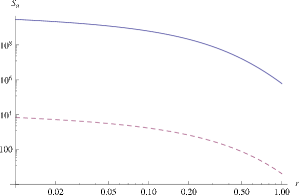
Figure 8: Comparing spatial auto-correlations of velocity, when $q=1.5$, between magnetic (solid line) and non-magnetic (dashed line) flows.

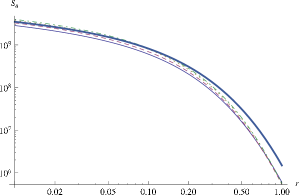
Figure 9: Spatial auto-correlations of velocity, when $q=1.5$ (solid line), $1.7$ (dashed line), $1.9$ (dotted line), $1.9999$ (dotdashed line) and flow is nonrotating (thick-solid line).

Like the discussions of temporal correlations, here also we begin by comparing the results between magnetic and non-magnetic flows, as shown in Figure 8. This again confirms that the magnetic field creates an additional effect leading to a much larger growth of perturbation.

Figure 9 shows that the spatial correlations of velocity perturbation in magnetized flows decrease with the decrease of $q$ from $1.9999$, while the difference between those of any two $q$s is insignificant. Note that the nonrotating case gives a slightly larger correlation than all the rotating cases. It is generally seen that the correlations decrease with increasing $r$ as well. However, their value appears significant enough to reveal a steadily damped instability in the flow. Such large values of perturbation energy growth are indicative of instability and plausible turbulent transport, in the presence of stochastic noise.

Figure 10 shows all spatial auto-correlations for a magnetized Keplerian disk. Like the temporal case, velocity correlation is lowest and its curl, i.e. the vorticity correlation, is highest. The underlying reasons being similar as described in the case of temporal correlations, when the existence of modulation due to Alfvén wave plays a determining rule. However, all the correlations are large enough to reveal instability.

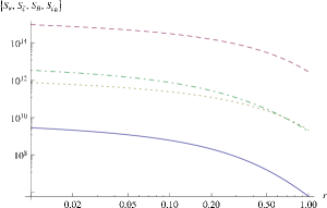
Figure 10: Spatial auto-correlations of velocity (solid line), vorticity (dashed line), magnetic field (dotted line), magnetic vorticity (dot-dashed line), when $q=1.5$.

III.2.2 Cross-Correlations

Here we stick to the same assumptions as of the computations of auto-correlations. We can define the spatial cross-correlation of two quantities, e.g. $u$ and $\zeta$, as

$$<u(\vec{x},t)\,\zeta(\vec{x}+\vec{r},t)>=S_{u\zeta}(r)=\int d^{3}k\,d\omega\,e^{i\vec{k}.\vec{r}}<\tilde{u}_{\vec{k},\omega}\,\tilde{\zeta}_{-\vec{k},-\omega}>.$$ (33)

Similarly, one can define other cross-correlations.

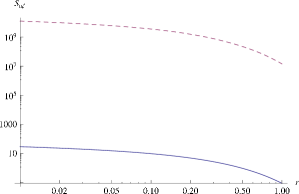
Figure 11: Comparing spatial cross-correlations of velocity and vorticity, when $q=1.5$, between magnetic (solid line) and non-magnetic (dashed line) flows.

Figure 11 further confirms that the cross-correlations can behave in the opposite fashion in the presence of magnetic field, compared to the auto-correlation. The reason being the same as that discussed in order to describe the temporal cross-correlations.

Figure 12 shows all spatial cross-correlations for a magnetized Keplerian disk, which is in accordance with auto-correlations described in Figure 10 and the description for temporal cross-correlations.

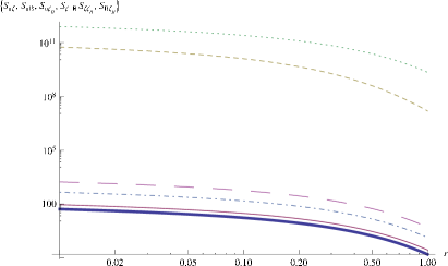
Figure 12: Spatial cross-correlations of velocity and vorticity (thick solid line), velocity and magnetic field (solid line), velocity and magnetic vorticity (dashed line), vorticity and magnetic field (dotted line), vorticity and magnetic vorticity (dot-dashed line), magnetic field and magnetic vorticity (long dashed line), when $q=1.5$.

IV Two-point correlations of perturbation in the presence of colored noise

Here we show, how the effects of colored noise change the correlations, mainly their amplitudes. For this purpose, we stick to a particular background profile which corresponds to the Keplerian disk. We consider the colored noise in such a way that the correlation function $D_{i}$ scales as $1/k^{3-\alpha}$. Then we choose three values of $\alpha$, which are $3$ (white noise), $2$ and $0$ (no vertex correction). In Figures 13 and 14, we compare effects of various colored noise to the temporal and spatial auto-correlations respectively. Further, in Figures 15 and 16, we compare effects of various colored noise to a typical (velocity and magnetic field) temporal and spatial cross-correlations respectively. The figures clearly show that effects of colored noise decrease the correlations — larger the magnitudes of slop of $D_{i}$, smaller the correlations are. However, even for $D_{i}\sim k^{-3}$, auto-correlations are large enough to govern instability.

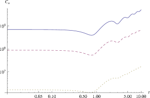
Figure 13: Temporal auto-correlations of velocity for $q=1.5$, when $D_{i}=k^{0}$ (solid line), $k^{-1}$ (dashed line), $k^{-3}$ (dotted line).

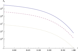
Figure 14: Spatial auto-correlations of velocity for $q=1.5$, when $D_{i}=k^{0}$ (solid line), $k^{-1}$ (dashed line), $k^{-3}$ (dotted line).

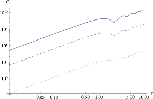
Figure 15: Temporal cross-correlations of velocity and magnetic field for $q=1.5$, when $D_{i}=k^{0}$ (solid line), $k^{-1}$ (dashed line), $k^{-3}$ (dotted line).

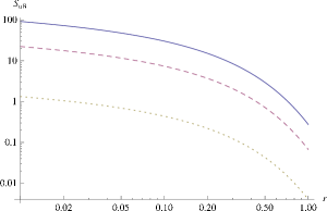
Figure 16: Spatial cross-correlations of velocity and magnetic field for $q=1.5$, when $D_{i}=k^{0}$ (solid line), $k^{-1}$ (dashed line), $k^{-3}$ (dotted line).

V Summary and conclusions

In this work, we have attempted to address the origin of instability and then turbulence in magnetized, rotating, shear flows (more precisely a small section of it, which is a plane shear flow supplemented by the Coriolis force). Our particular emphasis is the flows having decreasing angular velocity but increasing specific angular momentum with the radial coordinate, which are Rayleigh stable. The flows with such a kind of velocity profile are often seen in astrophysics. As the molecular viscosity in astrophysical accretion disks is negligible, any transport of matter therein would arise through turbulence only, in order to explain observed data. Therefore, essentially we have addressed here the plausible origin of viscosity in rotating shear flows of the kind mentioned above. Note that whether a flow is magnetically arrested or not, hydrodynamic effects always exist, as Mukhopadhyay & Chattopadhyay mc13 argued. Hence, the relative strengths of hydrodynamics and hydromagnetics in the time scale of interest determines the actual source of instability. Present work shows that the strength of hydromagnetic effects could be superior than that of hydrodynamic effects.

We have shown, based on the theory of statistical physics (which has been recalled in detail by Mukhopadhyay & Chattopadhyay mc13 , in the present context), that stochastically forced linearized rotating shear flows in a narrow gap limit reveal a very large correlation energy growth of perturbation in the presence of magnetic field and noise. We have shown separately (1) the sole effects of magnetic field at fixed noise and rotation, (2) sole effects of rotation at fixed magnetic field and noise, and (3) sole effects of noise at fixed magnetic field and rotation.

Although the correlations of perturbation decrease as the flow deviates from the type with $q=1.9999$ (when $q=2$ exactly corresponds to constant specific angular momentum) to that of the Keplerian, the difference between them is very small and they appear large enough to trigger nonlinear effects and instability.

Therefore, the present work addresses the large three-dimensional hydromagnetic energy growth of linear perturbation, in the line with theoretical framework grounded by Mukhopadhyay & Chattopadhyay mc13 , which presumably leads to instability and subsequent turbulence. Only requirement here is the presence of stochastic noise and magnetic field in the system together, which is quite obvious in natural flows like astrophysical (hot) accretion disks around compact objects. Interestingly, all the flows with $q<2$, exhibiting very similar growth and roughness exponents with almost identical energy dissipation amplitudes, indicates the universality class. In addition, all the correlations tend to saturate at a large time. This feature is clearer in the log-linear plots given by Figures 17 and 18. It is known that the time for maximum transient growths arised in a non-normal system, like the one under consideration, scales as $R_{e}^{\gamma}$, when $\gamma\geq 0$ man . As $R_{e}$ and $R_{m}$ are chosen to be very large in the present work, in practical time scales the correlations never reveal any transient behavior. Note that, at large $r$, all the spatial correlations reveal similar amplitude as well. Thus the properties of temporal and spatial correlations together, in the presence of noise and magnetic field, indicate that the Rayleigh stable rotating shear flows follow a single universality class. Another aspect to be noted from our work is that the presence of magnetic field brings in oscillatory nature in the energy growths of the system (due to the presence of Alfvén wave), unlike the energy growths in hydrodynamic case mc13 . Therefore, there might be a possibility of existence of a flow in which the presence of magnetic field hinders the energy growth of perturbation instead of enhancing the same — a veritable destructive interference. This, however, has to be investigated in detail, in particular relaxing the choice of specific wave-vector of perturbations and also including dominant non-linear perturbing modes.

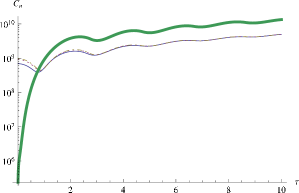
Figure 17: Temporal auto-correlations, in log-linear scale, of velocity, when $q=1.5$ (solid line), $1.9$ (dashed line), $1.9999$ (dotted line) and flow is nonrotating (thick-solid line).

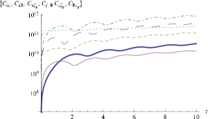
Figure 18: Temporal cross-correlations, in log-linear scale, of velocity and vorticity (thick solid line), velocity and magnetic field (solid line), velocity and magnetic vorticity (dashed line), vorticity and magnetic field (dotted line), vorticity and magnetic vorticity (dot-dashed line), magnetic field and magnetic vorticity (long dashed line), when $q=1.5$.

References

- (1) Mukhopadhyay, B., & Chattopadhyay, A. K., J. Phys. A 46, 035501 (2013)
- (2) Mukhopadhyay, B, Mathew, R., & Raha, S., NJPh 13, 023029 (2011)
- (3) Gu, P.-G., Vishniac, E. T., & Cannizzo, J. K., ApJ 534, 380 (2000)
- (4) Kim, W.-T., & Ostriker, E. C., ApJ 540, 372 (2000)
- (5) Mahajan, S. M., & Krishan, V., ApJ 682, 602 (2008)
- (6) Mukhopadhyay, B., Afshordi, N., & Narayan, R., ApJ 629, 383 (2005)
- (7) Rudiger, G., & Zhang, Y., A&A 378, 302 (2001)
- (8) Dauchot, O., & Daviaud, F., Phys. Fluids 7, 335 (1995)
- (9) Richard, D., & Zahn, J.-P., A&A 347, 734 (1999)
- (10) Klahr, H. H., & Bodenheimer, P., ApJ 582, 869 (2003)
- (11) Dubrulle, B., Dauchot, O., Daviaud, F., & Longaretti, P.-Y., Richard, D., & Zahn, J.-P., Phys. Fluids 17, 095103 (2005)
- (12) Dubrulle, B., Mari, L., Normand, C., Hersant, F., Richard, D., & Zahn, J.-P. A&A 249, 1 (2005)
- (13) Balbus, S. A., Hawley, J. F., & Stone, J. M., ApJ 467, 76 (1996)
- (14) Hawley, J. F., Balbus, S. A., & Winters, W. F., ApJ 518, 394 (1999)
- (15) Lesur, G., & Longaretti, P.-Y., A&A 444, 25 (2005)
- (16) Pumir, A., Phys. Fluids 8, 3112 (1996)
- (17) Fromang, S., & Papaloizou, J., A&A 476, 1113 (2007)
- (18) Paoletti, M. S., van Gils, D. P. M., Dubrulle, B., Sun, C., Lohse, D., & Lathrop, D. P., A&A 547, A64 (2012)
- (19) Avila, M., Phys. Rev. Lett. 108, 124501 (2012)
- (20) Eckhardt, B., & Pandit, R., Eur. Phys. J. B 33, 373 (2003)
- (21) Forster, D., Nelson, D. R., & Stephen, M. J., Phys. Rev. A 16, 732 (1977)
- (22) Chattopadhyay, A. K., & Bhattacharjee, J. K., Phys. Rev. E 63, 016306 (2000)
- (23) Barabási, A.-L. & Stanley, H. E., Fractal concepts in surface growth (Cambridge University Press, 1995)