Two-neutrino double-beta decay Fermi transition and two-nucleon interaction

Abstract

An exactly solvable model for a description of the two-neutrino double beta decay transition of the Fermi type is considered. By using perturbation theory an explicit dependence of the two-neutrino double beta decay matrix element on the like-nucleon pairing, particle-particle and particle-hole proton-neutron interactions by assuming a weak violation of isospin symmetry of Hamiltonian expressed with generators of the SO(5) group. It is found that there is a dominance of double beta decay transition through a single state of the intermediate nucleus. Then, an energy weighted sum rule connecting $\Delta$Z=2 nuclei is presented and discussed. It is suggested that this sum rule can be exploited to study the residual interactions of the nuclear Hamiltonian.

I Introduction

The two-neutrino double-beta decay ($2\nu\beta\beta$-decay), which involves the emission of two electrons and two antineutrinos doi83 ; haxton ; suci98 ; fs98 ; ves12

$$(A,Z)\rightarrow(A,Z+2)+2e^{-}+2{\tilde{\nu}}_{e},$$ (1)

has attracted the attention of both experimentalists and theoreticians for a long period and remains of major importance for nuclear physics.

It is a second order process in the weak interaction allowed in the standard model. The $2\nu\beta\beta$-decay can be observed, because due to the pairing force even-even nuclei with an even number of protons and neutrons are more stable than the odd-odd nuclei with broken pairs doi83 ; haxton . Thus, the single $\beta$-decay transition from the (A,Z) nucleus to neighboring odd-odd nucleus is energetically forbidden.

Till now, the $2\nu\beta\beta$-decay has been detected for 11 different nuclei for transition to the ground state and in two cases also to transition to $0^{+}$ excited state of the daughter nucleus recbb . This rare process is one of the major sources of background in running and planned experiments looking for a signal of the more fundamental neutrinoless double-beta decay, which occurs if the neutrino is a massive Majorana particle.

The inverse half-life of the $2\nu\beta\beta$-decay is free of unknown parameters of particle physics and can be factorized to a good approximation as doi83 ; haxton

$$\left(T^{2\nu}_{1/2}\right)^{-1}=G^{2\nu}g^{4}_{A}\left|M^{2\nu}_{GT}-\left(\frac{g_{V}}{g_{A}}\right)^{2}M^{2\nu}_{F}\right|^{2},$$ (2)

where $G^{2\nu}$ is the lepton phase-space factor, $g_{A}$ ($g_{V}$) is the axial-vector (vector) coupling constant. The $2\nu\beta\beta$-decay is governed by the double Gamow-Teller (GT) and double Fermi (F) matrix elements, which are given by doi83 ; haxton ; suci98 ; fs98

$$M^{2\nu}_{F,GT} = \sum_{n}\frac{\langle f\parallel{\cal O}_{F,GT}\parallel 1^{+}_{n}\rangle\langle 1^{+}_{n}\parallel{\cal O}_{F,GT}\parallel i\rangle}{E_{n}-(E_{i}+E_{f})/2}$$ (3)

with

$${\cal O}_{F}=\sum_{k=1}^{A}\tau^{+}_{k},~{}~{}~{}~{}~{}{\cal O}_{GT}=\sum_{k=1}^{A}\tau^{+}_{k}\boldmath{\sigma_{k}}.$$ (4)

where $|i>$ ($|f>$) are $0^{+}$ ground states of the initial (final) even-even nuclei with energy $E_{i}$ ($E_{f}$), and $|1^{+}_{n}>$ ($|0^{+}_{n}>$) are the $1^{+}$ ($0^{+}$) states in the intermediate odd-odd nucleus with energies $E_{n}$.

Many attempts have been made in the literature to calculate the $2\nu\beta\beta$-decay nuclear matrix elements (NMEs) for nuclei of experimental interest doi83 ; haxton ; suci98 ; fs98 ; domin ; rath07 ; sarr . Recent results obtained within the nuclear shell model are in a good agreement with the measured $2\nu\beta\beta$-decay half-lives poves12 . But, it is achieved by a consideration of significant quenching by a factor q=0.4-0.7 of the Gamow-Teller operator, which is obtained by a normalization of the total theoretical $\beta^{-}$ strength in the experimental energy window to the measured one.

The quasiparticle random phase approximation (QRPA) has been found to be successful in revealing the suppression mechanism for the $2\nu\beta\beta$-decay NMEs vogel86 ; civitarese87 ; muto89 . However, the predictive power of the QRPA is questionable because of extreme sensitivity of calculated $2\nu\beta\beta$-decay matrix elements in the physically acceptable region on the particle-particle strength of nuclear Hamiltonian. In muto89 it was shown that if this strength is determined from a QRPA calculation of single $\beta^{+}$ decays a reasonable agreement with the measured $2\nu\beta$-decay is achieved.

The quenching behavior of the $2\nu\beta\beta$-decay matrix elements is a puzzle and has attracted the attention of many theoreticians. Recently, it was shown that $M^{2\nu}_{F}$ depends strongly on the isovector part of the particle-particle neutron-proton interaction unlike $M^{2\nu}_{GT}$, which depends strongly on its isoscalar part newpar13 . The underlying symmetries responsible for these suppressions are assumed to be isospin SU(2) and spin-isospin SU(4) symmetries in the cases of double Fermi and double Gamow-Teller NMEs, respectively desplan90 .

The goal of this paper is to discuss the suppression mechanism of the double Fermi matrix element close to the point of restoration of isospin symmetry of the nuclear Hamiltonian in the context of residual nucleon-nucleon interaction. For the sake of simplicity we consider a schematic Hamiltonian, describing the gross properties of the beta-decay processes in the simplest case of monopole Fermi transitions within the SO(5) model kuzmin ; muto92 ; civi94 ; hplb ; hirsch97 ; krmpotic98 . In order to find explicit dependence of $M^{2\nu}_{F}$ on different parts of the nuclear Hamiltonian the perturbation theory is exploited. We note that the SO(5) model remains a tool for understanding of different nuclear physics phenomena even nowadays engel04 ; anatomy ; engel12 .

II Schematic Hamiltonian within the SO(5) model

In the model, protons and neutrons occupy only a single j-shell. The Hamiltonian includes a single-particle term, proton-proton and neutron-neutron pairing, and a charge-dependent two-body interaction with both particle-hole and particle-particle channels as follows:

$$H = e_{p}N_{p}+e_{n}N_{n}-G_{p}S_{p}^{\dagger}S_{p}-G_{n}S_{n}^{\dagger}S_{n}$$ (5)

$$+ 2\chi\beta^{-}\beta^{+}-2\kappa P^{-}P^{+},$$

where

$$N_{i}=\sum_{m}a^{\dagger}_{m,t_{i}}a^{\phantom{\dagger}}_{m,t_{i}},\quad\beta^{-}=\sum_{m}a^{\dagger}_{m,-\frac{1}{2}}a^{\phantom{\dagger}}_{m,\frac{1}{2}},$$

$$S_{i}^{\dagger}=\frac{1}{2}\sum_{m}a^{\dagger}_{m,t_{i}}{\tilde{a}}^{\dagger}_{m,t_{i}},\quad P^{-}=\sum_{m}a^{\dagger}_{m,-\frac{1}{2}}{\tilde{a}}^{\dagger}_{m,\frac{1}{2}},$$

with i=p, n and $t_{n,p}=\pm 1/2$. $a^{\dagger}_{mt}$ ($a_{mt}$) is creation (annihilation) operator of single particle state $|jm,t>$ for protons and neutrons ($t=t_{p},t_{n}$) and ${\tilde{a}}^{\dagger}_{mt}=(-1)^{j-m}a^{\dagger}_{-mt}$.

We rewrite Hamiltonian (5) with help of operators

$$A^{\dagger}\left(T_{z}\right)=\frac{1}{\sqrt{2}}\left[a^{\dagger}\otimes a^{\dagger}\right]^{1}_{T_{z}},$$

$$N=N_{p}+N_{n},\quad T_{z}=\frac{N_{n}-N_{p}}{2},$$

$$T^{-}=-\sqrt{2\Omega}\sum_{m}a^{\dagger}_{m,-\frac{1}{2}}a^{\phantom{\dagger}}_{m,\frac{1}{2}}.$$ (7)

Here, $A^{\dagger}\left(T_{z}\right)$ is the nucleon pair creation operator with angular momentum $J=0$, isospin $T=1$ and its projection on z-axis $T_{z}$ ($T_{z}=0,\pm 1$). $N$, $T_{z}$ and $T^{-}$ are the particle-number operator, the isospin projection and the isospin lowering operators, respectively. It holds the identity $T^{2}=\left(T^{-}T^{+}+T^{+}T^{-}\right)/2+T_{z}^{2}$. $\Omega=j+1/2$ denotes the semi-degeneracy of the considered single level. The operators (7) with their Hermitian conjugates represent ten generators of the SO(5) group parikh . We assume, the system is in seniority s=0. Then, $[A^{{}^{\dagger}}\tilde{A}]_{0}^{0}$ expressed with the SO(5) Casimir operator parikh is given by

$$[A^{{}^{\dagger}}\tilde{A}]_{0}^{0}=\frac{1}{2\sqrt{3}\Omega}\left[\left(2\Omega+3-N/2\right)N/2-T(T+1)\right].$$ (8)

For the Hamiltonian (5) we get

$$H = \left[e_{n}+e_{p}-\frac{1}{3}\left(3+2\Omega-\frac{N}{2}\right)\left(\frac{G_{p}+G_{n}}{2}+2\kappa\right)\right]\frac{N}{2}+\left[e_{n}-e_{p}-2\chi(T_{z}+1)\right]T_{z}$$ (9)

$$+\left[2\chi+\frac{1}{3}\left(\frac{G_{p}+G_{n}}{2}+2\kappa\right)\right]T(T+1)$$

$$+\frac{\Omega}{\sqrt{2}}\left(\frac{G_{p}-G_{n}}{2}\right)[A^{{}^{\dagger}}\tilde{A}]^{1}_{0}+\sqrt{\frac{2}{3}}\Omega\left(4\kappa-\frac{G_{p}+G_{n}}{2}\right)[A^{{}^{\dagger}}\tilde{A}]^{2}_{0}.$$

As a consequence of the presence of the isovector and isoquadrupole terms in Hamiltonian (9) the isospin is not conserved in general. It is due to differences between proton and neutron pairing strengths and an arbitrary strength of the proton-neutron isovector pairing component. However, particle number and isospin projection remains as good quantum numbers.

The k^th eigenstates of the Hamiltonian (9) with quantum numbers N and T_z can be expressed in terms of a basis labeled by a chain of irreducible representations of the SO(5) group (see Appendix A), namely

$$|k;NT_{z}\rangle=\sum_{T}c^{(k)}_{NTT_{z}}|NTT_{z}\rangle.$$ (10)

A diagonalization of H requires calculation of matrix elements $\left\langle N,T,T_{Z}\right|H\left|N,T,T_{Z}\right\rangle$ and $\left\langle N,T\pm 2,T_{Z}\right|H\left|N,T,T_{Z}\right\rangle$. The corresponding reduced matrix elements are given Appendix A). For $G_{p}=G_{n}$ and $(G_{p}+G_{n})/2=4\kappa$ the Hamiltonian (9) is diagonal in the basis of states $|N,T,T_{z}\rangle$.

III Double Fermi matrix element within perturbation theory

We shall assume a small violation of the isospin symmetry due to isotensor term of nuclear Hamiltonian (9). For the numerical example we consider a large value of j to simulate the realistic situation corresponding to medium- and heavy-mass nuclei. The parameters chosen are given by

$$\begin{array}[]{ccc}\Omega=10,&N=20,&1\leq T_{z}\leq 5,\\ e_{p}=0.3~{}\text{MeV},&e_{n}=0.1~{}\text{MeV},&G=0.165~{}\text{MeV},\\ G_{p}=G_{n}=G,&\chi=0.044~{}\text{MeV},&0.7\leq 4\kappa/G\leq 1.3.\end{array}$$ (11)

For $4\kappa/G=1$ the isospin symmetry is restored. In Fig. 1 we present $0^{+}$ states with energy $E_{TT_{z}}$ of different isotopes. This level scheme illustrates the situation for the $2\nu\beta\beta$-decay of ⁴⁸Ca. The isospin is known to be, to a very good approximation, a valid quantum number in nuclei. The ground states of ⁴⁸Ca and ⁴⁸Ti can be identified with T=4 $T_{z}=4$ and T=2 $T_{z}=2$, respectively, i.e. they are assigned into different isospin multiplets. As the total isospin projection lowering operator $T^{-}$ is not changing the isospin the double Fermi matrix element $M^{2\nu}_{F}$ is non-zero only to the extent that the Coulomb interaction mixes the high-lying T=4 $T_{z}$=2 analog of the ⁴⁸Ca ground state into the T=2 $T_{z}=2$ ground state of ⁴⁸Ti.

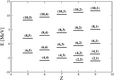
Figure 1: The energy of the $0^{+}$ states of different isotopes are shown for j=19/2 (and the set of parameters (11) with $4\kappa/G=1$) in MeV vs. Z plot. States are labeled by $\left(T,T_{z}\right)$.

We shall study double Fermi matrix element in the perturbation theory within the discussed model close to a point of a restoration of the isospin symmetry ($4\kappa/G=1$). The isoscalar and isotensor terms of the Hamiltonian (9) represent the unperturbated and perturbated terms, respectively. We denote perturbated states and their energies with a superscript prime symbol ($|T^{\prime}T_{z}\rangle$, $E^{\prime}_{TT_{z}}$) unlike the states with a definite isospin ($|TT_{z}\rangle$, $E_{TT_{z}}$). Up to the second order of parameter $(4\kappa-G)$ we find

$$E^{\prime}_{44} = 14e_{n}+6e_{p}-\frac{110}{3}\left(G+2\kappa\right)$$ (12)

$$-\sqrt{\frac{2}{3}}\Omega\left(G-4\kappa\right)\left\langle 44\right|[A^{{}^{\dagger}}\tilde{A}]_{0}^{2}\left|44\right\rangle$$

$$-\frac{2}{3}\Omega^{2}\left(G-4\kappa\right)^{2}\frac{\left\langle 64\right|[A^{{}^{\dagger}}\tilde{A}]_{0}^{2}\left|44\right\rangle^{2}}{44\chi+22/3\left(G+2\kappa\right)},$$

$$E^{\prime}_{43} = 13e_{n}+7e_{p}+16\chi-\frac{110}{3}\left(G+2\kappa\right)$$ (13)

$$-\sqrt{\frac{2}{3}}\Omega\left(G-4\kappa\right)\left\langle 43\right|[A^{{}^{\dagger}}\tilde{A}]_{0}^{2}\left|43\right\rangle$$

$$-\frac{2}{3}\Omega^{2}\left(G-4\kappa\right)^{2}\frac{\left\langle 63\right|[A^{{}^{\dagger}}\tilde{A}]_{0}^{2}\left|43\right\rangle^{2}}{44\chi+22/3\left(G+2\kappa\right)},$$

$$E^{\prime}_{22} = 12e_{n}+8e_{p}-\frac{124}{3}\left(G+2\kappa\right)$$ (14)

$$-\sqrt{\frac{2}{3}}\Omega\left(G-4\kappa\right)\left\langle 22\right|[A^{{}^{\dagger}}\tilde{A}]_{0}^{2}\left|22\right\rangle$$

$$-\frac{2}{3}\Omega^{2}\left(G-4\kappa\right)^{2}\frac{\left\langle 42\right|[A^{{}^{\dagger}}\tilde{A}]_{0}^{2}\left|22\right\rangle^{2}}{28\chi+14/3\left(G+2\kappa\right)},$$

$$E^{\prime}_{42} = 12e_{n}+8e_{p}+28\chi-\frac{110}{3}\left(G+2\kappa\right)$$ (15)

$$-\sqrt{\frac{2}{3}}\Omega\left(G-4\kappa\right)\left\langle 42\right|[A^{{}^{\dagger}}\tilde{A}]_{0}^{2}\left|42\right\rangle$$

$$+\frac{2}{3}\Omega^{2}\left(G-4\kappa\right)^{2}\frac{\left\langle 42\right|[A^{{}^{\dagger}}\tilde{A}]_{0}^{2}\left|22\right\rangle^{2}}{28\chi+14/3\left(G+2\kappa\right)}$$

$$-\frac{2}{3}\Omega^{2}\left(G-4\kappa\right)^{2}\frac{\left\langle 62\right|[A^{{}^{\dagger}}\tilde{A}]_{0}^{2}\left|42\right\rangle^{2}}{44\chi+22/3\left(G+2\kappa\right)}.$$

The particular matrix elements of SO(5) operators connecting states with a definite isospin and its projection are presented in Appendix A).

For transition $|4^{\prime}4>\rightarrow|2^{\prime}2>$ the double Fermi matrix element can be written as

$$M^{2\nu}_{F}=\sum_{T=4,6,8,10}^{10}\frac{\left\langle 2^{\prime}2\right|T^{-}\left|T^{\prime}3\right\rangle\left\langle T^{\prime}3\right|T^{-}\left|4^{\prime}4\right\rangle}{E^{\prime}_{T3}-\left(E^{\prime}_{44}-E^{\prime}_{22}\right)/2}.$$ (16)

It contains a sum over the states of the intermediate nucleus $|T^{\prime}3\rangle$. However, up to second order of perturbation theory there is only a single contribution through the intermediate state $|4^{\prime}3\rangle$. Thus, we have

$$M^{2\nu}_{F}\simeq\frac{\left\langle 2^{\prime}2\right|T^{-}\left|4^{\prime}3\right\rangle\left\langle 4^{\prime}3\right|T^{-}\left|4^{\prime}4\right\rangle}{E^{\prime}_{33}-\left(E^{\prime}_{44}-E^{\prime}_{22}\right)/2}.$$ (17)

The involved $\beta$-transition amplitudes are given by

$$\left\langle 4^{\prime}3\right|T^{-}\left|4^{\prime}4\right\rangle = \left\langle 43\right|T^{-}\left|44\right\rangle\left(1-\frac{1}{3}\frac{\Omega^{2}\left(4\kappa-G\right)^{2}}{\left(44\chi+22/3\left(G+2\kappa\right)\right)^{2}}\left[\left|\left\langle 44\right|[A^{{}^{\dagger}}\tilde{A}]_{0}^{2}\left|64\right\rangle\right|^{2}+\left|\left\langle 43\right|[A^{{}^{\dagger}}\tilde{A}]_{0}^{2}\left|63\right\rangle\right|^{2}\right]\right)$$

$$+\left\langle 63\right|T^{-}\left|64\right\rangle\frac{2}{3}\frac{\Omega^{2}\left(4\kappa-G\right)^{2}}{\left(44\chi+22/3\left(G+2\kappa\right)\right)^{2}}\left\langle 64\right|[A^{{}^{\dagger}}\tilde{A}]_{0}^{2}\left|44\right\rangle\left\langle 63\right|[A^{{}^{\dagger}}\tilde{A}]_{0}^{2}\left|43\right\rangle$$

and

$$\left\langle 2^{\prime}2\right|T^{-}\left|4^{\prime}3\right\rangle = \left\langle 42\right|T^{-}\left|43\right\rangle\left[\sqrt{\frac{2}{3}}\Omega\left(G-4\kappa\right)\frac{\left\langle 42\right|[A^{{}^{\dagger}}\tilde{A}]_{0}^{2}\left|22\right\rangle}{\left(28\chi+14/3\left(G+2\kappa\right)\right)}\right.$$

$$+\left.\frac{2}{3}\frac{\Omega^{2}\left(G-4\kappa\right)^{2}}{\left(28\chi+14/3\left(G+2\kappa\right)\right)^{2}}\left(\left\langle 42\right|[A^{{}^{\dagger}}\tilde{A}]_{0}^{2}\left|42\right\rangle\left\langle 42\right|[A^{{}^{\dagger}}\tilde{A}]_{0}^{2}\left|22\right\rangle-\left\langle 22\right|[A^{{}^{\dagger}}\tilde{A}]_{0}^{2}\left|22\right\rangle\left\langle 42\right|[A^{{}^{\dagger}}\tilde{A}]_{0}^{2}\left|22\right\rangle\right)\right].$$

If isospin symmetry is restored ($4\kappa=G$) we end up with $\left\langle 2^{\prime}2\right|T^{-}\left|4^{\prime}3\right\rangle=\left\langle 22\right|T^{-}\left|43\right\rangle=0$. For the energy denominator in (17) with help of Eqs. (12), (13) and (14) we get

$$E^{\prime}_{43}-\left(E^{\prime}_{44}-E^{\prime}_{22}\right)/2=16\chi+\frac{7}{3}\left(G+2\kappa\right)$$ (20)

$$+\sqrt{\frac{1}{6}}\Omega\left(4\kappa-G\right)\left[2\left\langle 43\right|[A^{{}^{\dagger}}\tilde{A}]_{0}^{2}\left|43\right\rangle-\left\langle 44\right|[A^{{}^{\dagger}}\tilde{A}]_{0}^{2}\left|44\right\rangle-\left\langle 22\right|[A^{{}^{\dagger}}\tilde{A}]_{0}^{2}\left|22\right\rangle\right]$$

$$+\frac{1}{3}\Omega^{2}\left(4\kappa-G\right)^{2}\left[\frac{\left\langle 64\right|[A^{{}^{\dagger}}\tilde{A}]_{0}^{2}\left|44\right\rangle^{2}}{44\chi+22/3\left(G+2\kappa\right)}+\frac{\left\langle 42\right|[A^{{}^{\dagger}}\tilde{A}]_{0}^{2}\left|22\right\rangle^{2}}{28\chi+14/3\left(G+2\kappa\right)}-2\frac{\left\langle 63\right|[A^{{}^{\dagger}}\tilde{A}]_{0}^{2}\left|43\right\rangle^{2}}{44\chi+22/3\left(G+2\kappa\right)}\right]$$

We note that the energy denominator $E^{\prime}_{43}-\left(E^{\prime}_{44}-E^{\prime}_{22}\right)/2$ as well as the whole double Fermi matrix element $M^{2\nu}_{F}$ does not depend explicitly on mean field parameters $e_{p}$ and $e_{n}$.

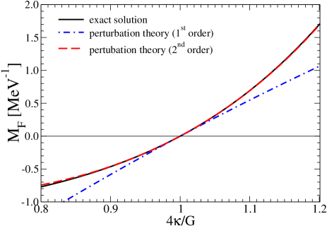
Figure 2: (Color online) Matrix element $M^{2\nu}_{F}$ for the double-Fermi two-neutrino double-beta decay mode as function of the ratio $4\kappa/G$ for a set of parameters (11). Exact results are indicated with a solid line. The results obtained within the perturbation theory up to the first and second order in isotensor contribution to Hamiltonian are shown with dash-dotted and and dashed lines, respectively. The restoration of isospin symmetry is achieved for $4\kappa/G=1$.

If we restrict our consideration to the first order perturbation theory, for transition $|4^{\prime}4>\rightarrow|2^{\prime}2>$ the double Fermi matrix element can be written as

$$M^{2\nu}_{F} \simeq \frac{\left\langle 42\right|T^{-}\left|43\right\rangle\left\langle 43\right|T^{-}\left|44\right\rangle}{16\chi+\frac{7}{3}\left(G+2\kappa\right)}\times$$ (21)

$$\sqrt{\frac{2}{3}}\Omega\left(G-4\kappa\right)\frac{\left\langle 42\right|[A^{{}^{\dagger}}\tilde{A}]_{0}^{2}\left|22\right\rangle}{\left(28\chi+14/3\left(G+2\kappa\right)\right)}.$$

In Fig. (2) $M^{2\nu}_{F}$ is plotted as function of ratio $4\kappa/G$. We see that results obtained with the second order perturbation theory agree well with exact results within a large range of this parameter. We note also that close to a point of restoration of isospin symmetry ($4\kappa/G=1$) a consideration of the first order perturbation theory seems to be sufficient, in particular for $M^{2\nu}_{F}\leq 0.3$.

IV Energy weighted sum rule of $\Delta$Z=2 nuclei

We suggest that a quantity relevant for the $2\nu\beta\beta$-decay might be the energy weighted double Fermi (or Gamow-Teller) sum rule associated with $\Delta$Z=2 nuclei:

$$S^{ew}_{F,GT}(i,f)$$

$$=\sum_{n}(E_{n}-\frac{E_{i}+E_{f}}{2})\left\langle f\right|{\cal O}_{F,GT}\left|n\right\rangle\left\langle n\right|{\cal O}_{F,GT}\left|i\right\rangle$$

$$=\frac{1}{2}\left\langle f\right|\left[{\cal O}_{F,GT},\left[H,{\cal O}_{F,GT}\right]\right]\left|i\right\rangle.$$ (22)

Here, $|i>$ and $|f>$ are assumed to be a ground state of the initial and a ground state or an excited state of the final nuclei participating in double-beta decay. If there is a dominance of contribution of a single or few states of the intermediate nucleus the left-hand side of Eq. (IV) might be determined phenomenologically. Then, by a calculation of the right-hand side of Eq. (IV) within a nuclear model the strengths of the residual interaction of Hamiltonian can be properly adjusted. We note that as the double commutator connect states with $\Delta$Z=2 the explicit dependence on single-particle part of nuclear Hamiltonian is eliminated unlike it is in the case of energy weighted sum rules related to a single nuclear ground state. We note that the energy weighted double Gamow-Teller sum rule associated with the $2\nu\beta\beta$-decay was discussed within the proton-neutron QRPA in vadim05 ; vadim11 .

We analyze the above sum rule for Fermi transitions and Hamiltonian (9) with $G_{p}=G_{n}$ within the SO(5) model. By rewriting the Hamiltonian as

$$H = (e_{p}+e_{n})N/2+(e_{p}-e_{n})T_{z}+2\chi T^{-}T^{+}$$ (23)

$$- 2G\Omega\left(A^{{}^{\dagger}}(-1)A(-1)+A^{{}^{\dagger}}(1)A(1)\right)$$

$$- 4\kappa\Omega A^{{}^{\dagger}}(0)A(0)$$

and exploiting the commutation relations of the SO(5) group (A) we find

$$S^{ew}_{F}(i,f)=\frac{1}{2}\left\langle f\right|\left[T^{-},\left[H,T^{-}\right]\right]\left|i\right\rangle$$

$$=2\Omega(G-4\kappa)\left\langle i\right|[A^{{}^{\dagger}}\tilde{A}]_{2}^{2}\left|f\right\rangle+2\chi\left\langle f\right|T^{-}T^{-}\left|i\right\rangle.$$

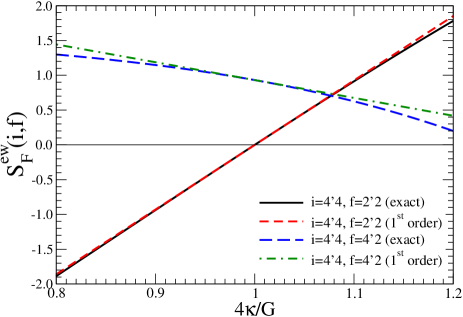
Figure 3: (Color online) The energy weighted sum rule $S^{ew}_{F,GT}(i,f)$ (IV) for two sets of states ($i=4^{\prime}4$, $f=2^{\prime}2$ and $i=4^{\prime}4$, $f=4^{\prime}2$) as function of the ratio $4\kappa/G$ for a set of parameters (11). The exact results are compared with those obtained within the first order perturbation theory.

i) The case $\left|i\right\rangle=\left|4^{\prime}4\right\rangle$, $\left|f\right\rangle=\left|2^{\prime}2\right\rangle$. We have

$$S^{ew}_{F}(4^{\prime}4,2^{\prime}2)$$

$$=\sum_{T^{\prime}}(E^{\prime}_{T3}-\frac{E^{\prime}_{44}+E^{\prime}_{22}}{2})\left\langle 2^{\prime}2\right|T^{-}\left|T^{\prime}3\right\rangle\left\langle T^{\prime}3\right|T^{-}\left|4^{\prime}4\right\rangle$$

$$=2\Omega(G-4\kappa)\left\langle 4^{\prime}4\right|[A^{{}^{\dagger}}\tilde{A}]_{2}^{2}\left|2^{\prime}2\right\rangle+2\chi\left\langle 2^{\prime}2\right|T^{-}T^{-}\left|4^{\prime}4\right\rangle.$$

If the first order perturbation theory is applied to any of two expressions for energy weighted sum rule in (IV) we find

$$S^{ew}_{F}(4^{\prime}4,2^{\prime}2)\simeq\left(16\chi+\frac{7}{3}\left(G+2\kappa\right)\right)\times$$

$$\sqrt{\frac{2}{3}}\Omega\left(G-4\kappa\right)\frac{\left\langle 42\right|[A^{{}^{\dagger}}\tilde{A}]_{0}^{2}\left|22\right\rangle}{\left(28\chi+14/3\left(G+2\kappa\right)\right)}\times$$

$$\left\langle 42\right|T^{-}\left|43\right\rangle\left\langle 43\right|T^{-}\left|44\right\rangle.$$ (26)

By comparing this expression with Eqs. (III), (III) and (20) we see that only the lowest intermediate state $|4^{\prime}3>$ contributes to the sum rule within the considered approximation. We find again a combination of energies of involved states to be a function of pairing, particle-particle and particle-hole interactions: $E^{\prime}_{43}-(E^{\prime}_{44}+E^{\prime}_{22})/2\simeq 16\chi+\frac{7}{3}\left(G+2\kappa\right)$.

ii) The case $\left|i\right\rangle=\left|4^{\prime}4\right\rangle$, $\left|f\right\rangle=\left|4^{\prime}2\right\rangle$. The energy weighted sum rule is given by

$$S^{ew}_{F}(4^{\prime}4,4^{\prime}2)$$

$$=\sum_{T^{\prime}}(E^{\prime}_{T3}-\frac{E^{\prime}_{44}+E^{\prime}_{42}}{2})\left\langle 4^{\prime}2\right|T^{-}\left|T^{\prime}3\right\rangle\left\langle T^{\prime}3\right|T^{-}\left|4^{\prime}4\right\rangle$$

$$=2\Omega(G-4\kappa)\left\langle 4^{\prime}4\right|[A^{{}^{\dagger}}\tilde{A}]_{2}^{2}\left|4^{\prime}2\right\rangle+2\chi\left\langle 4^{\prime}2\right|T^{-}T^{-}\left|4^{\prime}4\right\rangle.$$

Within the first order perturbation theory we find

$$S^{ew}_{F}(4^{\prime}4,4^{\prime}2)\simeq\left(2\chi+\right.$$

$$\sqrt{1/6}\Omega(4\kappa-G)\left[2\left\langle 43\right|[A^{{}^{\dagger}}\tilde{A}]_{0}^{2}\left|43\right\rangle\right.$$

$$\left.\left.-\left\langle 44\right|[A^{{}^{\dagger}}\tilde{A}]_{0}^{2}\left|44\right\rangle-\left\langle 42\right|[A^{{}^{\dagger}}\tilde{A}]_{0}^{2}\left|42\right\rangle\right]\right)$$

$$\left\langle 42\right|T^{-}\left|43\right\rangle\left\langle 43\right|T^{-}\left|44\right\rangle.$$ (28)

We note that the dominant contribution to $S^{ew}_{F}(4^{\prime}4,4^{\prime}2)$ comes from the transition through the single intermediate state $|43^{\prime}>$ again. For a combination of energies of involved states we have

$$E^{\prime}_{43}-(E^{\prime}_{44}+E^{\prime}_{42})/2=$$

$$2\chi+\sqrt{1/6}\Omega(4\kappa-G)\left(2\left\langle 43\right|[A^{{}^{\dagger}}\tilde{A}]_{0}^{2}\left|43\right\rangle\right.$$

$$\left.-\left\langle 44\right|[A^{{}^{\dagger}}\tilde{A}]_{0}^{2}\left|44\right\rangle-\left\langle 42\right|[A^{{}^{\dagger}}\tilde{A}]_{0}^{2}\left|42\right\rangle\right).$$ (29)

Thus, the energy weighted sum rule $S^{ew}_{F}(4^{\prime}4,4^{\prime}2)$ implies another useful relation between energies of states and nucleon-nucleon interactions.

In Fig. 3 two different energy weighted sum rules associated with final states $|2^{\prime}2>$ and $|4^{\prime}2>$ are plotted as function of the ratio $4\kappa/G$ for a considered set of parameters (11). They exhibit different dependence on $4\kappa/G$. It is because the final state $|4^{\prime}2>$ belongs ($|2^{\prime}2>$ does not belong) to the same isospin multiplet as the initial nucleus. We see a very good agreement between the exact results and results obtained within the first order perturbation theory, which allows only the lowest intermediate state $|4^{\prime}3>$ to contribute to a sum rule. A better agreement would be achieved if the corresponding combination of energies of states would evaluated up to the second order perturbation theory. We note that a contribution from the second lowest intermediate state to the sum rules $S^{ew}_{F}(4^{\prime}4,2^{\prime}2)$ and $S^{ew}_{F}(4^{\prime}4,4^{\prime}2)$ appears only in the third order perturbation theory.

V Conclusions

An exactly solvable model for the description of the $2\nu\beta\beta$-decay processes of the Fermi type was used to discuss the dependence of the double-beta decay matrix element $M^{2\nu}_{F}$ on different components of the residual interaction, namely like-nucleon pairing, particle-particle and particle hole proton-neutron interactions. We note that the model is equivalent to a complete shell-model treatment in a single-j shell for the adopted Hamiltonian. In addition, it reproduces the main features of the results obtained in realistic calculations.

Good isospin forbids the $2\nu\beta\beta$-decay. One needs an isotensor force to mix $\Delta$T = 2. Naturally, the Coulomb interaction contains such a isotensor force. In our case we break isospin symmetry by hand. The only isospin violation comes from the difference of the proton-proton ($G_{p}$) and the neutron-neutron ($G_{n}$) pairing force compared to the proton-neutron isospin = 1 pairing force ($\kappa$). By taking the advantage of the perturbation theory up to the second order in the isotensor contribution to the Hamiltonian a dominance of a contribution through a single state of the intermediate nucleus to $M^{2\nu}_{F}$ and explicite dependence of $M^{2\nu}_{F}$ on different types of nucleon-nucleon interactions was found. The mean-field part of Hamiltonian does not enter explicitly in this decomposition of double Fermi matrix element and is related only to the calculation of unperturbated states of Hamiltonian.

Further, the importance of the energy weighted sum rule associated with $\Delta$Z=2 nuclei for fitting different components of residual interaction of the Hamiltonian was pointed out. It goes without saying that a further studies, in particular by considering realistic nuclear Hamiltonian and Gamow-Teller transitions, are of great interest.

Appendix A The SO(5) algebra and matrix elements

Following parikh we introduce operators of the SO(5) group, which are expressed with operators (7) as follows:

$$\begin{array}[]{cc}H_{1}=N/2-\Omega,&H_{2}=T_{Z},\\ E_{11}=\sqrt{\Omega}A^{\dagger}(1),&E_{-1-1}=\sqrt{\Omega}A(1),\\ E_{1-1}=-\sqrt{\Omega}A^{\dagger}(-1),&E_{-11}=-\sqrt{\Omega}A(-1),\\ E_{10}=\sqrt{\Omega}A^{\dagger}(0),&E_{-10}=\sqrt{\Omega}A(0),\\ E_{01}=\frac{1}{2}\sqrt{2}T^{+},&E_{0-1}=\frac{1}{2}\sqrt{2}T^{-},\\ \end{array}$$ (35)

Their commutation relations are parikh

$$\left[H_{1},H_{2}\right]=0,\quad\left[H_{1},E_{ab}\right]=aE_{ab},$$

$$\left[H_{2},E_{ab}\right]=bE_{ab},$$

$$[E_{ab},E_{-a-b}]=aH_{1}+bH_{2}$$

and

$$[E_{ab},E_{a^{\prime}b^{\prime}}]=\pm E_{a+a^{\prime}b+b^{\prime}},$$ (36)

if $a+a^{\prime}=0,\pm 1$ and $b+b^{\prime}=0,\pm 1$. Otherwise, $[E_{ab},E_{a^{\prime}b^{\prime}}]=0$.

For the present task, states with with seniority s=0 are considered. Thus, it is sufficient to define them with quantum numbers N, T and T_z. They are constructed with help of the isospin lowering operator T^- on the state $|{\rm N,T,T_{z}=T}\rangle$, which is given by parikh

$$\left|NTT\right\rangle = N(a,b)O^{a}_{+}O^{b}_{00}\left|N=4\Omega,T=T_{z}=0\right\rangle,$$

with

$$O_{+} = E_{-11},$$

$$O_{00} = 2E_{-11}E_{-1-1}+E_{-10}E_{-10}$$ (37)

$O_{+}$ reduces the number of particles by two units and increases the isospin by one unit and $O_{00}$ reduces the number of particles by four units. $a$ and $b$ are integers:

$$a=T,~{}~{}~{}~{}~{}~{}b=\Omega-\frac{T}{2}-\frac{N}{4}.$$ (38)

From a construction of the states it follows that a difference in isospin of two states with fixed $N,T_{z}$ is an even number.

The reduced matrix elements are calculated with help of the Wigner-Eckart theorem in the convention as follows:

$$\left\langle T^{\prime}T_{z}^{\prime}\left|T^{p}_{q}\right|TT_{z}\right\rangle=C^{T^{\prime}T_{z}^{\prime}}_{TT_{z}pq}\left\langle T^{\prime}\left|\left|T^{p}\right|\right|T\right\rangle$$ (39)

Particular Clebsh-Gordan coefficients of interest are given by va

$$C_{TT_{z}20}^{TT_{z}}=\frac{3T_{z}^{2}-T(T+1)}{\sqrt{(2T-1)T(T+1)(2T+3)}}$$

$$C_{TT_{z}20}^{T+2T_{z}}=\sqrt{\frac{3(T+T_{z}+1)(T+T_{z}+2)(T-T_{z}+1)(T-T_{z}+2)}{(2T+1)(2T+2)(2T+3)(T+2)}}$$

We present relevant reduced matrix elements, which agree with those of hirsch97 up to few corrections:

$$\left\langle T+2\left|\left|[A^{{}^{\dagger}}\tilde{A}]^{2}\right|\right|T\right\rangle=-\frac{1}{2\Omega}\sqrt{\frac{\left(T+2\right)\left(T+N/2+3\right)\left(2\Omega-T-N/2\right)\left(T+1\right)\left(N/2-T\right)\left(2\Omega+T-N/2+3\right)}{\left(2T+3\right)\left(2T+5\right)}}$$

$$\left\langle T\left|\left|[A^{{}^{\dagger}}\tilde{A}]^{2}\right|\right|T\right\rangle = \frac{1}{\sqrt{6}C^{TT}_{TT20}}\left[\left\langle NTT\left|A^{{}^{\dagger}}(1)A(1)\right|NTT\right\rangle+\left\langle NTT\left|A^{{}^{\dagger}}(-1)A(-1)\right|NTT\right\rangle\right.$$

$$- \left.2\left\langle NTT\left|A^{{}^{\dagger}}(0)A(0)\right|NTT\right\rangle\right]$$

$$\left\langle T\left|\left|[A^{{}^{\dagger}}\tilde{A}]^{1}\right|\right|T\right\rangle=\frac{1}{\sqrt{2}C^{TT}_{TT10}}\left[\left\langle NTT\left|A^{{}^{\dagger}}(-1)A(-1)\right|NTT\right\rangle-\left\langle NTT\left|A^{{}^{\dagger}}(1)A(1)\right|NTT\right\rangle\right]$$

$$\left\langle NTT\left|A^{{}^{\dagger}}(1)A(1)\right|NTT\right\rangle=\frac{1}{\Omega}\left[-\Omega+T+N/2+\frac{\left(2\Omega-T-N/2\right)\left(T+N/2+3\right)\left(T+1\right)}{2\left(2T+3\right)}\right]$$

$$\left\langle NTT\left|A^{{}^{\dagger}}(-1)A(-1)\right|NTT\right\rangle=\frac{1}{\Omega}\left[\frac{\left(2\Omega+T-N/2+3\right)\left(-T+N/2\right)\left(T+1\right)}{2\left(2T+3\right)}\right]$$

$$\left\langle NTT\left|A^{{}^{\dagger}}(0)A(0)\right|NTT\right\rangle= \frac{1}{\Omega}\left[-\Omega+N/2+\frac{\left(2\Omega-T-N/2\right)\left(T+N/2+3\right)\Omega}{\left(2\Omega+T-N/2+1\right)\left(-T+N/2+2\right)}\times\right.$$ (40)

$$\left.\left\langle N+4TT\left|A^{{}^{\dagger}}(0)A(0)\right|N+4TT\right\rangle\right]$$

The matrix element on the right hand side of Eq. (40) can be calculated recurrently by keeping in mind that for $N_{max}=4\Omega-2T$ we have

$$\left\langle N_{max}TT\left|A^{{}^{\dagger}}(0)A(0)\right|N_{max}TT\right\rangle=1-T/\Omega$$

For isospin raising (lowering) operators the Condon Shortley convention is assumed:

$$T^{\pm}\left|N,T,T_{z}\right\rangle=\sqrt{\left(T\pm T_{z}+1\right)\left(T\mp T_{z}\right)}\left|N,T,T_{z}\pm 1\right\rangle.$$

References

(1) M. Doi, T. Kotani, and E. Tagasugi, Prog. Theor. Phys. (Supp.) 83, 1 (1985).