Robustness and Directed Structures in Ecological Flow Networks
Abstract
Robustness of ecological flow networks under random failure of arcs is considered with respect to two different functionalities: coherence and circulation. In our previous work, we showed that each functionality is associated with a natural path notion: lateral path for the former and directed path for the latter. Robustness of a network is measured in terms of the size of the giant laterally connected arc component and that of the giant strongly connected arc component, respectively. We study how realistic structures of ecological flow networks affect the robustness with respect to each functionality. To quantify the impact of realistic network structures, two null models are considered for a given real ecological flow network: one is random networks with the same degree distribution and the other is those with the same average degree. Robustness of the null models is calculated by theoretically solving the size of giant components for the configuration model. We show that realistic network structures have positive effect on robustness for coherence, whereas they have negative effect on robustness for circulation.
Introduction
Networks have been usually considered as undirected in the field of complex networks (Newman,, 2003). However, many real-world networks are directed so that the direction of interaction is important for the functioning of the systems. Recently, it has been revealed that directed networks have richer structures such as directed assortativity (Foster et al.,, 2010) and flow hierarchy (Mones,, 2013).
In our previous work, we proposed a new path notion involving directedness called lateral path that can be seen as the dual notion to the usual directed path (Haruna,, 2011). Based on category theoretic formulation, we derived the lateral path as a natural path notion associated with the dynamic mode of biological networks: a network is a pattern constructed by gluing functions of entities constituting the network (Haruna,, 2012). Thus, its functionality is coherence, whereas the functionality of the directed path is transport. We showed that there is a division of labor with respect to the two functionalities within a network for several types of biological networks: gene regulation, neuronal and ecological ones (Haruna,, 2012). It was suggested that the two complementary functionalities are realized in biological systems by making use of the two ways of tracing on a directed network, namely, lateral and directed.
In this paper, we address robustness of ecological flow networks with respect to the lateral path and directed path, respectively. Since the natural connectedness notion associated with the directed path is the strong connectedness, we consider robustness of the giant strongly connected component (GSCC) for the latter. For the former, robustness of the giant lateral connected component (GLCC) is of interest. Thus, we assess robustness of ecological flow networks in terms of two different functionalities, namely, coherence and circulation, both of which are important for the functioning of them (Ulanowicz,, 1997).
Robustness of ecological networks is an intriguing issue in recent studies (Montoya et al.,, 2006; Bascompte,, 2009). Initially, robustness of general complex networks has been argued qualitatively in terms of critical thresholds for the existence of the giant component (Albert et al.,, 2000; Cohen et al.,, 2001). For ecological networks, their robustness has been measured by the size of secondary extinctions (Solé and Montoya,, 2001; Dunne et al.,, 2002). Here, we employ a recently proposed idea to measure robustness quantitatively (Schneider et al.,, 2011; Herrmann et al.,, 2011). As a first step, we consider only random failure of arcs. The size of giant components is measured by the number of arcs involved because laterally connected components are defined only on the set of arcs.
Here, we study the impact of realistic network structures on robustness with respect to the two functionalities. Two complementary measures of it are proposed by comparing the robustness of a given real network with that of the two null models: random networks with the same degree distribution and those with the same average degree. The robustness of the two null models is calculated by theoretically solving the percolation problem on the configuration model, random networks with an arbitrary degree distribution (Newman et al.,, 2001).
This paper is organized as follows. In Section 2, we develop a theory to calculate the size of GLCC and GSCC under random removal of arcs in the configuration model. In Section 3, we propose two measure for the impact of realistic structures on robustness of networks by using the theoretical result obtained in Section 2. In Section 4, the proposed measures are applied to 10 ecological flow networks. In Section 5, we discuss the results and indicate future directions.
Random Removal of Arcs in the Configuration Model
In this section, we consider a percolation problem, random removal of arcs, in the configuration model with respect to the lateral connectedness and the strong connectedness.
A lateral path in a directed network is a path in the network such that the direction of arcs involved changes alternately (Haruna,, 2012) (Fig. 1). Two arcs are called laterally connected if they are connected by a lateral path (Haruna,, 2011). Lateral connectedness defines an equivalence relation on the set of arcs. Each equivalence class is called laterally connected component.

Since lateral connectedness is defined on the set of arcs, here we also consider strong connectedness for arcs. Two arcs are called strongly connected if there is a directed path from one arc to the other arc, and vice versa.
Let us consider a random directed network with degree distribution . is the fraction of nodes in the network with in-degree and out-degree . We make use of the generating function formalism (Callaway et al.,, 2000; Newman et al.,, 2001) to calculate the sizes of giant laterally or strongly connected components (in short, GLCC or GSCC, respectively) after removing arcs uniformly at random with probability , where is the occupation probability.
The generating function for is
| (1) |
The average degree is given by
| (2) |
Let be the in-degree distribution and the out-degree distribution. Their generating functions are
| (3) |
respectively.
We introduce four excess degree distributions and corresponding generating functions that are necessary for the calculation in what follows.
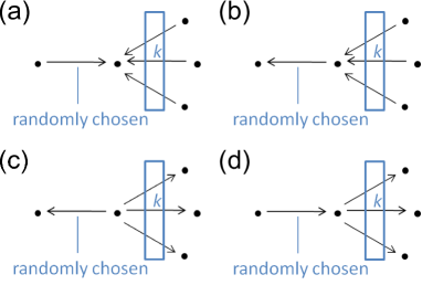
First, let be the probability that the number of the other arcs arriving at the target node of a randomly chosen arc is (Fig. 2 (a)). It is given by
| (4) |
and its generating function is
| (5) |
Second, let be the probability that the number of arcs arriving at the source node of a randomly chosen arc is (Fig. 2 (b)). It is given by
| (6) |
and its generating function is
| (7) |
Third, let be the probability that the number of the other arcs leaving from the source node of a randomly chosen arc is (Fig. 2 (c)). It is given by
| (8) |
and its generating function is
| (9) |
Finally, let be the probability that the number of arcs leaving from the target node of a randomly chosen arc is (Fig. 2 (d)). It is given by
| (10) |
and its generating function is
| (11) |

Giant Laterally Connected Component
Let be the average probability that an arc is not connected to the GLCC via a particular arc with the same target and the average probability that an arc is not connected to the GLCC via a particular arc with the same source. Then, the average probability that an occupied arc does not belong to the GLCC is
| (12) |
Hence, the size of the GLCC is
| (13) |
The values of and are calculated by the following set of equations:
| (14) |
The critical occupation probability for the appearance of GLCC can be obtained from the linear stability analysis of the trivial solution of (14). It turns out to be
| (15) |
Giant Strongly Connected Component
The calculation of the size of the GSCC is similar to the node component case (Dorogovtsev et al.,, 2001; Schwartz et al.,, 2002). In (Serrano and De Los Rios,, 2007), five notions of edge components are considered. For our purpose, consideration on the usual three components (in-, out- and strongly connected) as in the node component case are enough. However, these are implicit in the following calculation.
Let be the average probability that an arc is not connected to the GSCC via a particular arc leaving from its target and the average probability that an arc is not connected to the GSCC via a particular arc arriving at its source. Then, the average probability that an occupied arc does belong to the GSCC is
| (16) |
Hence, the size of the GSCC is
| (17) |
The values of and are calculated by the following set of equations:
| (18) |
The critical occupation probability for the appearance of GSCC is given by
| (19) |
which is the same as in the node component case (Schwartz et al.,, 2002).

Examples
We calculate the sizes of the GLCC and the GSCC as functions of the occupation probability for three degree distributions: (a) Uncorrelated Poisson distribution (UPD)
| (20) |
(b) Uncorrelated exponential distribution (UED)
| (21) |
and (c) Correlated Poisson distribution (CPD)
| (22) |
where are parameters and is the Kronecker delta. The results are compared with numerical simulations in Fig. 3, which shows that the agreement between simulation and theory is well.
For critical occupation probabilities, we have for UPD, for UED and for CPD. Thus, these examples also show that all possibilities , and actually occur.
Two Measures for Impact of Realistic Structures on Robustness
Robustness
Given a directed network, let be the size of the GLCC and the size of the GSCC for occupation probability . Motivated by the robustness measure proposed in (Schneider et al.,, 2011; Herrmann et al.,, 2011), we define the robustness of the GLCC and that of the GSCC by
| (23) |
respectively.
Our robustness measure is similar to link robustness in (Zeng and Liu,, 2012), however, since we measure the size of a component by the number of arcs belonging to it, it is different from link robustness. In particular, since and cannot exceed the diagonal line, we have .
Gain
Given a directed network, we would like to consider how much its robustness (of the GLCC or the GSCC) is enhanced or degraded compared to a reference network. One measure is the ratio of the robustness of the given network to that of the reference network (Schneider et al.,, 2011). We call this measure robustness gain. If we denote the robustness of the given network by and that of the reference network by , then the robustness gain is defined by
| (24) |
We here consider three combinations of given-reference pairs: (given,ref)=(real, config), (given,ref)=(config, Poisson) and (given,ref)=(real,Poisson), where ‘real’ indicates a real-world network, ‘config’ the configuration model network with the same degree distribution and ‘Poisson’ the (uncorrelated) Poissonian network with the same average degree. The robustness gains for the three given-reference pairs are denoted by and , respectively. Note that .
Complement Ratio
The other way to measure the effect of realistic structures on robustness is to evaluate the amount of unrealized robustness of the reference network (namely, ) utilized by the given network. We define the robustness complement ratio for the above three combinations of given-reference pairs by
| (25) |
where , or .
Both and are considered for the lateral connectedness and the strong connectedness in next section. We write and for the former and and for the latter.
Ecological Flow Networks
In this section, we apply the indexes introduced in previous section to relatively large 10 networks (with the number of arcs ) among 48 flow networks collected by R. Ulanowicz. Data are downloaded from http://www.cbl.umces.edu/~ulan/ntwk/network.html.


Data
Here, we list the 10 ecological flow networks we analyze. In the following, is the number of nodes and is the number of arcs included in the largest weakly connected component. is the average degree. The number associated to each network is the web number in the original data source. In every network, each arc indicates the existence of carbon flow from its source to target. (i) Chesapeake Bay Mesohaline Network (, Web 34). (ii) Everglades Graminoids Wet Season (, Web 40). (iii) Final Narragansett Bay Model (, Web 42). (iv) Florida Bay Wet Season (, Web 38). (v) Lake Michigan Control Network (, Web 47). (vi) Lower Chesapeake Bay in Summer (, Web 46). (vii) Middle Chesapeake Bay in Summer (, Web 45). (viii) Mondego Estuary - Zostrea Site (, Web 41). (ix) St Marks River (Florida) Estuary (, Web 43). (x) Upper Chesapeake Bay in Summer (, Web 44).
Results
We plot (Fig. 4 (a)) and (Fig. 4 (b)) for (vii) Middle Chesapeake Bay in Summer network, the configuration model network with the same degree distribution and the Poissonian network with the same average degree, as a typical example. and for real ecological flow networks are calculated by averaging the size of the largest connected components over 1000 random removal sequences of arcs.
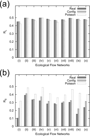
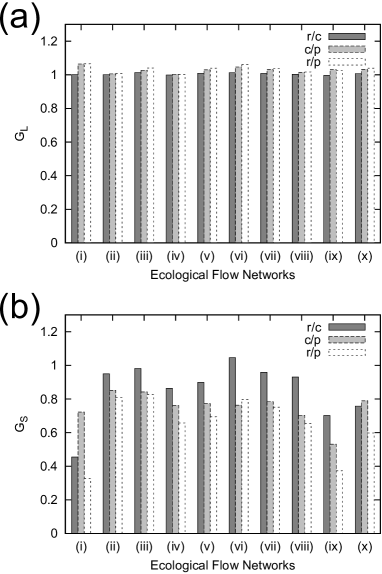
The robustness values for all 10 networks are shown in Fig. 5. One can see opposite tendency on how realistic structures influence robustness between the GLCC and the GSCC. tends to increase as more realistic structures are imposed on one hand, tends to decrease on the other hand. However, since is close to 0.5 already for the Poissonian network in most cases, the robustness gain for the GLCC is almost unity in all three given-reference pairs as seen in Fig. 6 (a). For , one can see that the realistic degree distributions are the dominant factor for the degradation of robustness in most cases from Fig. 6 (b).
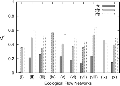
The tendency that realistic structures have positive impact on robustness of the GLCC can be captured more clearly by the robustness complement ratio as shown in Fig. 7. One can also see that the realistic degree distributions are the dominant factor to enhance the robustness of the GLCC in most cases.
Discussions
Whether realistic structures of ecological networks have positive impact on their robustness or stability or not is controversial (Allesina and Tang,, 2012). The answer to this question generally depends on the types of ecological interaction and dynamic processes of interest (Thébault and Fontaine,, 2010; Allesina and Tang,, 2012). In this paper, we focused on robustness of ecological flow networks under random failure of arcs with respect to the two different functionalities, namely, coherence and circulation. The former is captured by the robustness of the GLCC and the latter by that of the GSCC. We found that they exhibit opposite tendency for constraints by the realistic network structures: the realistic network structures enhance the robustness of the GLCC on one hand, they degrade that of the GSCC on the other hand. In both case, it is suggested that the realistic degree distributions are one of the most important factors.
The former result seems to be consistent with the food-web stabilizing factor proposed in (Gross et al.,, 2009): “(i) species at high trophic levels feed on multiple prey species and (ii) species at intermediate trophic levels are fed upon by multiple predator species”, because such patterns in a network could contribute to make multiple lateral paths between arcs. Whereas, the latter result could provide a quantitative support for the ‘autocatalytic view’ on ecological flow networks proposed by R. Ulanowicz (Ulanowicz,, 1997).
Our result in this paper suggests that complex networks can be both robust and fragile in a different sense from that in (Albert et al.,, 2000): under the same attack strategy, robust for one functionality and fragile for another functionality.
It is of interest whether the same tendency can be seen or not for the other various attack strategies (Holme and Kim,, 2002) and for the other kinds of directed biological networks such as gene regulation and brain. Research results on these issues will be reported elsewhere near future.
Acknowledgements
This work was partially supported by JST PRESTO program.
References
- Albert et al., (2000) Albert, R., Jeong, H., and Barabási, A.-L. (2000). Error and attack tolerance of complex networks. Nature, 406:378–382.
- Allesina and Tang, (2012) Allesina, S. and Tang, S. (2012). Stability criteria for complex ecosystems. Nature, 483:205–208.
- Bascompte, (2009) Bascompte, J. (2009). Disentangling the web of life. Science, 325:416–419.
- Callaway et al., (2000) Callaway, D. S., Newman, M. E. J., Strogatz, S. H., and Watts, D. J. (2000). Network robustness and fragility: percolation on random graphs. Phys. Rev. Lett., 85:5468–5471.
- Cohen et al., (2001) Cohen, R., Erez, K., ben Avraham, D., and Havlin, S. (2001). Breakdown of the internet under intentional attack. Phys. Rev. Lett., 86:3682–3685.
- Dorogovtsev et al., (2001) Dorogovtsev, S. N., Mendes, J. F. F., and Samukhin, A. N. (2001). Giant strongly connected component of directed networks. Phys. Rev. E, 64:025101(R).
- Dunne et al., (2002) Dunne, J. A., Williams, R. J., and Martinez, N. D. (2002). Network structure and biodiversity loss in food webs: robustness increases with connectance. Ecology Letters, 5:558–567.
- Foster et al., (2010) Foster, J. G., Foster, D. V., Grassberger, P., and Paczuski, M. (2010). Edge direction and the structure of networks. Proc. Natl. Acad. Sci. USA, 107:10815–10820.
- Gross et al., (2009) Gross, T., Rudolf, L., Levin, S. A., and Dieckmann, U. (2009). Generalized models reveal stabilizing factors in food webs. Science, 325:747–750.
- Haruna, (2011) Haruna, T. (2011). Global structure of directed networks emerging from a category theoretical formulation of the idea gobjects as processes, interactions as interfaces h. In Lenaerts, T., Giacobini, M., Bersini, H., Bourgine, P., Dorigo, M., and Doursat, R., editors, Advances in Artificial Life, ECAL 2011, Proceedings of the Eleventh European Conference on the Synthesis and Simulation of Living Systems, pages 310–317. MIT Press, Cambridge.
- Haruna, (2012) Haruna, T. (2012). Theory of interface: category theory, directed networks and evolution of biological networks. arXiv:1210.6166.
- Herrmann et al., (2011) Herrmann, H. J., Schneider, C. M., Moreira, A. A., Andrade Jr, J. S., and Havlin, S. (2011). Onion-like network topology enhances robustness against malicious attacks. J. Stat. Mech., P01027.
- Holme and Kim, (2002) Holme, P. and Kim, B. J. (2002). Attack vulnerability of complex networks. Phys. Rev. E, 65:056109.
- Mones, (2013) Mones, E. (2013). Hierarchy in directed random networks. Phys. Rev. E, 87:022817.
- Montoya et al., (2006) Montoya, J. M., Pimm, S. L., and Solé, R. V. (2006). Ecological networks and their fragility. Nature, 442:259–264.
- Newman, (2003) Newman, M. E. J. (2003). The structure and function of complex networks. SIAM Review, 45:167–256.
- Newman et al., (2001) Newman, M. E. J., Strogatz, S. H., and Watts, D. J. (2001). Random graphs with arbitrary degree distributions and their applications. Phys. Rev. E, 64:026118.
- Schneider et al., (2011) Schneider, C. M., Moreira, A. A., Andrade Jr, J. S., Havlin, S., and Herrmann, H. J. (2011). Mitigation of malicious attacks on networks. Proc. Natl. Acad. Sci. USA, 108:3838–3841.
- Schwartz et al., (2002) Schwartz, N., Cohen, R., ben Avraham, D., Barabási, A.-L., and Havlin, S. (2002). Percolation in directed scale-free networks. Phys. Rev. E, 66:015104(R).
- Serrano and De Los Rios, (2007) Serrano, M. A. and De Los Rios, P. (2007). Interfaces and the edge percolation map of random directed networks. Phys. Rev. E, 76:056121.
- Solé and Montoya, (2001) Solé, R. V. and Montoya, J. M. (2001). Complexity and fragility in ecological networks. Proc. R. Soc. Lond. B, 268:2039–2045.
- Thébault and Fontaine, (2010) Thébault, E. and Fontaine, C. (2010). Stability of ecological communities and the architecture of mutualistic and trophic networks. Science, 329:853–856.
- Ulanowicz, (1997) Ulanowicz, R. E. (1997). Ecology, the Ascendent Perspective. Columbia University Press, New York.
- Zeng and Liu, (2012) Zeng, A. and Liu, W. (2012). Enhancing network robustness against malicious attacks. Phys. Rev. E, 85:066130.