Chaos in the Kepler problem with quadrupole perturbations

Abstract

We use the Melnikov integral method to prove that the Hamiltonian flow on the zero-energy manifold for the Kepler problem perturbed by a quadrupole moment is chaotic, irrespective of the perturbation being of prolate or oblate type. This result helps to elucidate some recent conflicting works in the physical literature based on numerical simulations.

1 Introduction

The Kepler two-body problem has been a splendid inspiration for physicists and mathematicians for the last three centuries (see, for instance, Chapter 9 of kepler ). Many works, in particular, have been devoted to the study of the onset of chaos in the perturbed Kepler problem (see, for a recent review, JMP and the references therein). For astronomical and astrophysical applications, it is natural to consider the weak field approximation in which the gravitational field of a body is decomposed into a multipole expansion. The original Kepler problem corresponds to the case where only the first expansion term, the monopole, is present. The next term in the expansion, the dipole term, is known to give origin to integrable motion, see Chapter 7 of dipole and Section 2 below. The quadrupole term is usually considered as the simplest perturbation to the Newtonian potential which could lead to chaotic motion in the Kepler problem (see, for instance, GL ). By employing the usual cylindrical coordinates $(r,z,\phi)$ around the gravitational center, the simplest quadrupole perturbation to the Newtonian potential reads

$$U(r,z)=-\frac{\alpha}{\sqrt{r^{2}+z^{2}}}-\frac{q}{2}\frac{2z^{2}-r^{2}}{\left(r^{2}+z^{2}\right)^{5/2}},$$ (1)

where $\alpha$ and $q$ stands for, respectively, the monopole intensity (proportional to the total gravitational mass) and the quadrupole intensity. The cylindrical coordinates are assumed to be adjusted to the quadrupole direction. Two qualitative distinct cases can be distinguished for the potential (1). Oblate deformations, as those ones of rotating deformed bodies, corresponds to $q<0$, whereas prolate deformations, as cigar-like mass distributions, to $q>0$. The study of the integrability of a test body motion under action of the potential (1) is a long standing problem, with substantially relevance to astronomy and astrophysics BP .

In GL , a numerical study of bounded trajectories is reported suggesting that the motion under prolate perturbations would be indeed chaotic while, on the other hand, oblate perturbations would correspond to an integrable case. Such conclusion would be rather puzzling since it is known that, for disk-like perturbation (which could be understood as extreme oblate perturbations), bounded oblique orbits are known to be chaotic SV ; S . This qualitative differences for the cases $q>0$ and $q<0$ is attributed in GL to some qualitative differences in the saddle points of the effective potential, but it is also known that such kind of local argument leads typically to conditions that are not sufficient neither necessary to the appearance of chaos in theses systems AS . More recently, a new numerical study suggesting that the oblate perturbations would also give origin to bounded chaotic orbits has appeared LCF . Here, we explore these conflicting results by applying the Melnikov integral method Melnikov for the parabolic orbits revisited (the zero-energy manifold) of (1). We prove the quadrupole perturbations effectively give rise to chaotic motion on the zero-energy manifold, irrespective of the perturbation being of prolate $(q>0)$ or oblate $(q<0)$ type.

2 The Melnikov Conditions

The Hamiltonian associated to the motion of a test body of unit mass under the action of the potential (1) is given by

$$H=\frac{1}{2}\left(p_{r}^{2}+p_{z}^{2}\right)+\frac{L_{z}^{2}}{2r^{2}}+U(r,z),$$ (2)

where $(r,p_{r})$ and $(z,p_{z})$ stands for the usual canonical cylindrical coordinates and $L_{z}$ is the (conserved) angular momentum around the $z$ axis. The Hamiltonian $H$ is itself a conserved quantity and the integrability of the Hamiltonian flow governed by (2) corresponds to the celebrated problem of the existence of the third isolating conserved integral of motion BP . In order the write the quadrupole perturbation in (2) conveniently, let us introduce the new variables $(R,\theta)$

$$\left\{\begin{array}[]{l}r=R\cos\theta,\\ z=R\sin\theta,\end{array}\right.$$ (5)

which leads to

$$H=H_{0}+qW_{1}(R)+qW_{2}(R,\theta),$$ (6)

where

$$H_{0}=\frac{1}{2}\left(p_{R}^{2}+\frac{p_{\theta}^{2}}{R^{2}}\right)+\frac{L_{z}^{2}}{2R^{2}\cos^{2}\theta}-\frac{\alpha}{R},$$ (7)

with $(R,p_{R})$ and $(\theta,p_{\theta})$ standing for the usual canonical coordinates, and

$$-\frac{q}{R^{3}}+\frac{3q\cos^{2}\theta}{2R^{3}}\equiv qW_{1}(R)+qW_{2}(R,\theta).$$ (8)

Notice that the perturbation (8) corresponds to the case $\beta=3$ considered in JMP , but the unperturbed Hamiltonian (7) is indeed different. Without loss of generality, let us assume hereafter that $\alpha=1$. Notice that a dipole perturbation would give rise to a Hamiltonian (6) with $W_{1}=0$ and $W_{2}=R^{-2}\sin\theta$, which indeed corresponds to a particular case of the integrable case discussed in the Section 48 of dipole .

In order to compute the Melnikov integrals Melnikov for the Kepler problem with quadrupole perturbations, we will adopt the integral method adapted for parabolic orbits presented in revisited . To this purpose, we need to obtain the equivalent of the homoclinic orbit of our problem. The total energy and the total angular momentum are the conserved quantities of our system,

$${}H_{0}=\frac{\dot{R}^{2}}{2}+\frac{G^{2}}{2R^{2}}-\frac{1}{R},\\ {}G^{2}=R^{4}\dot{\theta}^{2}+\frac{L_{z}^{2}}{\cos^{2}\theta},$$ (9)

and from the expressions above, we have

$$\frac{dR}{\sqrt{2\left(H_{0}+\frac{1}{R}\right)-\frac{G^{2}}{R^{2}}}}=\pm dt{},\\ \frac{1}{R^{2}}\frac{dR}{\sqrt{2\left(H_{0}+\frac{1}{R}\right)-\frac{G^{2}}{R^{2}}}}=\frac{d\theta}{\sqrt{G^{2}-\frac{L_{z}^{2}}{\cos^{2}\theta}}},{}$$ (10)

From (LABEL:H_00), we see that the minimum value of $R$ with $H_{0}=0$ satisfies $G^{2}=2R_{min}$. We are interested in the parabolic orbits and, hence, substituting $H_{0}=0$ in (LABEL:eqn-r) and (LABEL:eqn-theta) and performing the integration, we have

$$\pm t=\frac{\sqrt{2}}{3}\left(R-\frac{R_{min}}{2}\right)\sqrt{R-R_{min}}+\rm{const}{},\\ \frac{1}{4A}\ln\left|\frac{A+\sin\theta}{A-\sin\theta}\right|+\rm{const}=\arctan\sqrt{\frac{R}{R_{min}}-1}.{}$$ (11)

where $A=\sqrt{1-\frac{L_{z}^{2}}{G^{2}}}$. Notice that, from (LABEL:G^2), one has that $0<A\leq 1$.

Inverting (LABEL:t_de_r), we have the expression $R(t)$ of the homoclinoc orbit, but this is not necessary to our purposes. Also, adjusting the constant in (LABEL:r_de_theta) so that $R=R_{min}$ for $\theta=0$, we have the following expression for $R(\theta)$

$$R(\theta)=R_{min}\sec^{2}\left[\frac{1}{4A}\ln\left|\frac{A+\sin\theta}{A-\sin\theta}\right|\right].$$ (12)

From (12), it is clear that $R(\theta)$ is an even function and that the parabolic orbit can be parametrized with $-\theta^{*}<\theta<\theta^{*}$, where $R(\theta^{*})=\infty$, which leads to

$$\sin\theta^{*}=A\tanh A\pi.$$ (13)

The Melnikov conditions to detect integrability of a Hamiltonian system of the type (2) corresponds to the existence of simple zeros for the quantities revisited

$$M_{1}(\theta_{0})=\int_{-\infty}^{\infty}\{H_{0},W_{2}\}\mathrm{d}t,\qquad M_{2}(\theta_{0})=\int_{-\infty}^{\infty}\{G,W_{2}\}\mathrm{d}t,$$ (14)

where the integrals are taken over the zero-energy manifold. For each value of $A$, this is a two-dimensional manifold parametrized as $\mathscr{R}=R(t-t_{0})$ and $\vartheta=\Theta(t-t_{0})+\theta_{0}$, with arbitrary $t_{0}$ and $\theta_{0}$. We see that

$$M_{1}(\theta_{0})=-\int_{-\infty}^{\infty}\left.\left[\dot{\mathscr{R}}\frac{\partial W_{2}}{\partial R}+\dot{\Theta}\frac{\partial W_{2}}{\partial\theta}\right]\mathrm{d}t=-W_{2}\right|_{t=-\infty}^{t=\infty}+\int_{-\infty}^{\infty}\frac{\partial W_{2}}{\partial t}\mathrm{d}t=0,$$ (15)

and, with some trigonometry, that

$$M_{2}(\theta_{0})=-\frac{3}{8R_{min}}\left[I_{1}\cos(2\theta_{0})+I_{2}\sin(2\theta_{0})\right],$$ (16)

where, after changing the integration variable,

$$I_{1}=\int_{-\theta^{*}}^{\theta^{*}}\frac{\sin(2\theta)}{R(\theta)}\mathrm{d}\theta,\qquad I_{2}=\int_{-\theta^{*}}^{\theta^{*}}\frac{\cos(2\theta)}{R(\theta)}\mathrm{d}\theta.$$ (17)

Since $R(\theta)$ is an even function, we have $I_{1}=0$. Finally, the non identically zero contribution to the Melnikov integral comes from the integral

$$I_{2}=\frac{1}{R_{min}}\int_{-\theta^{*}}^{\theta^{*}}\cos(2\theta)\cos^{2}\left[\frac{1}{4A}\ln\left|\frac{A+\sin\theta}{A-\sin\theta}\right|\right]\mathrm{d}\theta,$$ (18)

where $\theta^{*}$ is given by (13). Is is enough to prove that $I_{2}\neq 0$ for some value of $A$ to establish that $M_{2}(\theta_{0})$ given by (16) has (infinitely many) simple zeros, which implies the absence of the extra conserved integral of motion and, consequently, that the motion is indeed chaotic, irrespective of the sign of the perturbation parameter $q$. Figure 1 depicts the integral (18) as a function of $A$, and we can check that one has indeed $I_{2}\neq 0$ for $0<A<1$.

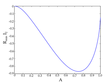
Figure 1: The integral (18) for different values of $A$. Notice that $I_{2}=0$ only for $A=0$ and for $A=1$, the latter corresponding to $L_{z}=0$ and, thus, to the case $\beta=3$ considered in JMP .

3 Final remarks

By using the Melnikov integral method adapted for parabolic orbits revisited , we prove that the Hamiltonian flow on the zero-energy manifold for the Kepler problem perturbed by a quadrupole moment is chaotic, irrespective of the perturbation being of prolate or oblate type. This result favors, in this way, the numerical results obtained in LCF , which are in conflict with those ones presented in GL .

- (1) R. Abraham and J.E. Marsden, Foundations of Mechanics, 2nd ed., AMS (2008).
- (2) F. Diacu, E. Pérez-Chavela, and M. Santoprete, J. Math. Phys. 46, 072701 (2005).
- (3) L.D. Landau and E.M. Lifshitz, Mechanics, Pergamon Press (1969).
- (4) E. Gueron and P.S. Letelier, Phys. Rev. E 63, 035201 (2001).
- (5) D. Boccalleti and G. Pucacco, Theory of Orbits. Volume 2: Perturbative and Geometrical Methods, Springer (2004).
- (6) A. Saa and R. Venegeroles, Phys. Lett. 259A 201 (1999).
- (7) A. Saa, Phys. Lett. 269A, 204 (2000).
- (8) A. Saa, Ann. Phys. (NY) 314, 508 (2004).
- (9) P.S. Letelier, J. Ramos-Caro, and F. López-Suspes, Phys. Lett. 375A, 3655 (2011).
- (10) P.J. Holmes and J.E. Marsden, J. Math. Phys 23, 669 (1982).
- (11) G. Cicogna and M. Santoprete, Regular and Chaotic Dynamics 6 377 (2001).