Triaxial Cosmological Haloes and the Disc of Satellites

Abstract

We construct simple triaxial generalisations of Navarro-Frenk-White haloes. The models have elementary gravitational potentials, together with a density that is cusped like $1/r$ at small radii and falls off like $1/r^{3}$ at large radii. The ellipticity varies with radius in a manner that can be tailored to the user’s specification. The closed periodic orbits in the planes perpendicular to the short and long axes of the model are well-described by epicyclic theory, and can be used as building blocks for long-lived discs.

As an application, we carry out the simulations of thin discs of satellites in triaxial dark halo potentials. This is motivated by the recent claims of an extended, thin disc of satellites around the M31 galaxy with a vertical rms scatter of $\sim 12$ kpc and a radial extent of $\sim 300$ kpc (Ibata et al. 2013). We show that a thin satellite disc can persist over cosmological times if and only if it lies in the planes perpendicular to the long or short axis of a triaxial halo, or in the equatorial or polar planes of a spheroidal halo. In any other orientation, then the disc thickness doubles on $\sim 5$ Gyr timescales and so must have been born with an implausibly small vertical scaleheight.

1 INTRODUCTION

This paper provides a family of flexible, triaxial, cosmologically inspired haloes. There is extensive evidence from numerical simulations that dark halos are well-represented by Navarro-Frenk-White (NFW) models with potential-density pair (see e.g., Mo, van den Bosch & White, 2010)

$$\rho_{\rm NFW}(r)={\rho_{0}{r_{\rm s}}^{3}\over r(r+{r_{\rm s}})^{2}},\qquad\psi_{\rm NFW}(r)=4\pi G\rho_{0}{{r_{\rm s}}^{3}\over r}\log(1+{r\over{r_{\rm s}}}).$$ (1)

Here, ${r_{\rm s}}$ and $\rho_{0}$ are the two parameters of the model providing a characteristic scalelength and density respectively. The parameters $\rho_{0}$ and ${r_{\rm s}}$ are known to be related by the mass-concentration relationship, albeit with some scatter (see e.g., Maccio et al., 2007).

Nonetheless, dark haloes are generically triaxial, whilst the NFW model is spherical. In purely collisionless simulations, dark haloes have typical axis ratios $b/a\sim 0.6$ and $c/a\sim 0.4$, where $c<b<a$ are the short, intermediate and long axes of the triaxial figure (see e.g., Jing & Suto, 2002; Allgood et al., 2006). When baryons are included, haloes remain triaxial, but tend to become rounder and more oblate, with typical ratios $b/a\sim 0.9$ and $c/a\sim 0.8$  (see e.g., Dubinski, 1994; Kazantzidis et al., 2004; Deason et al., 2011; Zemp et al., 2012). So, it would be useful to have a set of models based on the Navarro-Frenk-White potential, but which can be triaxial. The most obvious way of doing this is to take the expression for $\rho_{\rm NFW}(r)$ and replace $r^{2}$ by $m^{2}=x^{2}+y^{2}/p^{2}+z^{2}/q^{2}$, where ($x,y,z$) are Cartesians and $p=b/a$ and $q=c/a$ are the flattenings. This though leads to cumbersome quadratures for the gravitational potential, and so is unattractive for applications such as orbit integrations. The other obvious alternative of replacing $r^{2}$ by $m^{2}$ in the potential $\psi_{\rm NFW}(r)$ leads to models with negative mass, and so is still less desirable!

Here, we use a classical method that has been known since the nineteenth century. Spherical harmonics are eigenfunctions of the angular part of the Laplacian, and so provide a way of building simple and analytic potential-density pairs. This technique was popularised by Schwarzschild (1979) in his numerical models for triaxial elliptical galaxies, in which the spherical Hubble profile was modified by the addition of spherical harmonics. Subsequently, the technique was exploited by others, primarily with a view to understanding the intrinsic shapes of elliptical galaxies (see e.g., Hernquist & Quinn, 1989; de Zeeuw & Carollo, 1996; Schwarzschild, 1993). Here, we will exploit the technique to build triaxial dark haloes.

One reason to develop such models is to assess the longevity of structures in galaxy haloes. As a particular application, we study the recent claims of rotationally-supported discs of satellite galaxies in the M31 halo. This subject goes back at least as far as Fusi Pecci et al. (1995) who found early hints of discs of satellites. Subsequently, Koch & Grebel (2006) identified a near-polar great plane containing 9 satellites (M32, NGC 147, PegDIG, And I, And III, And V, And VI, And VII and And IX). They conjectured that this might be caused either by tidal break-up of a larger galaxy, or by preferential accretion along filaments or a prolate dark halo shape. The quality of the data has been substantially improved with the recent work of Conn et al. (2012, 2013). First, the detection efficiency of the survey was computed, allaying fears that selection biases may be contributing to the results. Second, the distances of the now more numerous satellites were derived by a Bayesian method applied to the Tip of the Red Giant Branch (TRGB). Conn et al. (2013) confirm the existence of a polar plane, now containing 15 satellites (Ands I, III, IX, XI, XII, XIII, XIV, XVI, XVII, XXV, XXVI, XXVII, NGC 147, NGC 185 and And XXX). Although the pole of the plane is $45^{\circ}$ away from that found by Koch & Grebel (2006), the commonality of some of the component satellites suggests that it may be the same structure. The plane is aligned with the Milky Way, and is orthogonal to the plane of the Milky Way disc. The root mean square (rms) scatter in distance from the plane is $\sim 12.6$ kpc. Subsequently, Ibata et al. (2013) analyzed the radial velocities of the satellites and came to a very remarkable conclusion. They argued that 13 of the 15 satellites possess a coherent, rotational motion. This, they suggested, is evidence of a gigantic structure, a vast rotating plane of satellites, nearly 400 kpc in extent, but very thin, with an rms scatter of 14.1 kpc at 99 % confidence level.

The claims of such a thin but extended disc of satellites around M31 are very surprising. Although the orbits of the satellites have periods of several Gyr, they are subject to torques from the quadrupole moment from the M31 bulge, disc and the triaxial dark halo. They also are subject to perturbing tidal forces from the nearby Milky Way galaxy. The orbital evolution driven by the combined effects of these forces might be expected to thicken any thin disc of satellites quite quickly. Of course, triaxial potentials can support closed periodic orbits in the planes perpendicular to the long and the short axis only. These are natural orbits on which cold gas or streams of satellite might settle and persist to give long-lived disc-like structures. However, even if located in such a propitious plane, it is far from clear that a thin disc of satellites could persist for long times.

The paper is arranged as follows. In Section 2, we develop triaxial halos models generalising the NFW potential. The closed orbits in the principal planes are found by epicyclic theory. Their properties are interesting as the orbits can potentially form the basis of long-lived discs. Section 3 describes our algorithm for seeding the initial conditions of orbits in extended discs in the outer parts of such halos, and analyses the results of such simulations. We show that, in general, a thin disc of satellites can be expected to double its thickness on timescales of $\sim 5$ Gyr. However, if the disc indeed lies in the planes perpendicular to the long or short axis of a triaxial halo, then it could survive and preserve its thinness over cosmological timescales.

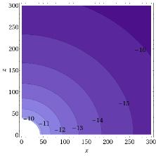
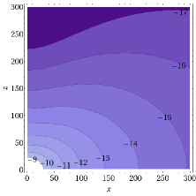
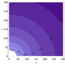
Figure 1: Comparison of isodensity surfaces using three popular ways of modelling asphericity. In the left panel, the density contours are elliptical, in the middle panel the equipotentials are elliptical and in the right panel the flattening is produced by spherical harmonics. (The contour labels are in logarithm of the density with units of $10^{10}M_{\odot}$ kpc^-3).

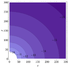
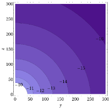
Figure 2: Contour plots of density in the principal planes of a triaxial Navarro-Frenk-White model. The $x$ axis is the longest, the $y$ axis the intermediate and the $z$ axis the shortest of the triaxial figure. The central value of the axis ratios are $p_{0}=(b/a)_{0}=0.9$ and $q_{0}=(c/a)_{0}=0.8$. At large radii, the model becomes rounder with axis ratios $p_{\infty}=(b/a)_{\infty}=0.95$ and $(c/a)_{\infty}=q_{\infty}=0.9$.

Model	Description	M31 mass	c	$q_{0}$	$q_{\infty}$	$p_{0}$	$p_{\infty}$	$\psi$	Milky Way	${t_{\rm h}}$	rms scatter
Number		(in $10^{12}M_{\odot}$)						(in deg)	Included ?	(in Gyr)	(in kpc)
1	Prolate	1.0	10.0	1.2	1.1	1.0	1.0	0.0	Yes	Stable	3.6
2	Oblate	1.0	10.0	0.8	0.9	1.0	1.0	90.0	Yes	Stable	4.8
3	Oblate	1.0	10.0	0.8	0.9	1.0	1.0	77.5	Yes	7.02	9.8
4	Oblate	1.0	10.0	0.8	0.9	1.0	1.0	45.0	No	5.47	19.4
5	Triaxial	1.0	10.0	0.8	0.9	0.9	0.95	90.0	No	Stable	3.6
6	Triaxial	1.0	10.0	0.8	0.9	0.9	0.95	77.5	No	6.99	9.4

Table 1: Properties of the models. The M31 halo has an NFW profile with mass $M$ and concentration $c$. The oblateness or prolateness is controlled by $q_{0}$ and $q_{\infty}$, whilst the triaxiality is controlled by $p_{0}$ and $p_{\infty}$. The angle of inclination of the disc of satellites to the pole ($z=0$) is given by $\psi$. So, for example, in model 2, 90^∘ means that the disc of satellites lies in the equatorial plane, while in model 3, $77^{\circ}$ means that the disc of satellites is coplanar with the stellar disc of M31. When the disc is unstable, then the e-folding time ${t_{\rm h}}$ is also given. The rms vertical scatter at the end of the simulation is recorded in kpc.

2 Dark Halo Models

For some applications, oblate or prolate NFW haloes suffice. So we deal with the simpler case in subsection 2.1, before passing to the triaxial case in subsection 2.2.

2.1 Oblate and Prolate Navarro-Frenk-White Halos

To provide a simple and flexible family of flattened halo models, we consider potentials of the form

$$\psi_{\rm axi}(r,\theta)=\psi_{\rm NFW}(r)-4\pi G{\rho_{1}r_{1}^{3}r\over(r+r_{1})^{2}}Y^{0}_{2}(\theta),$$ (2)

where ($r,\theta$) are spherical polar coordinates. $Y^{0}_{2}(\theta)=\frac{3}{2}\cos^{2}\theta-\frac{1}{2}$ is the familiar second spherical harmonic, which shortens (or lengthens) the $z$ axis of the density distribution, whilst lengthening (or shortening) the $x$ and $y$ axes to give an oblate (or prolate) figure. The flattened density is

$$\rho_{\rm axi}(r,\theta)=\rho_{\rm NFW}(r)-2\rho_{1}r_{1}^{3}{3r^{2}+8rr_{1}+2r_{1}^{2}\over r(r+r_{1})^{4}}Y^{0}_{2}(\theta).$$ (3)

Notice that the density still falls off like $r^{-1}$ at small radii and $r^{-3}$ at large radii, though this model is now oblate or prolate. There are two additional parameters $\rho_{1}$ and $r_{1}$, which control the normalisation and lengthscale of the asphericity and hence ellipticity of the density contours at large and small radii. We find

$${\rho_{0}{r_{\rm s}}^{3}\over\rho_{1}r_{1}^{3}}=3\Biggl{(}{2+q_{\infty}^{3}\over 1-q_{\infty}^{3}}\Biggr{)},$$ (4)

$${r_{1}^{2}\over{r_{\rm s}}^{2}}={2\over 3}\Biggl{(}{2+q_{0}\over 2+q_{\infty}^{3}}\Biggr{)}\Biggl{(}{1-q_{\infty}^{3}\over 1-q_{0}}\Biggr{)},$$ (5)

where $q_{0}$ and $q_{\infty}$ are the axis ratios of the isodensity contours near the center and at large radii. These formulae provide a simple way to fix the parameters of the model. First, $\rho_{0}$ and ${r_{\rm s}}$ are chosen to lie on the mass-concentration relationship derived from cosmological simulations (see e.g., Maccio et al., 2007). Then, $\rho_{1}$ and $r_{1}$ are chosen using eqns(4) and (5) to give the desired axis ratio near the centre $q_{0}$ and at large radii $q_{\infty}$.

Fig. 1 shows a comparison between the three popular ways of flattening a spherical model. Either the density or potential contours can be made elliptical (left and middle panels) or spherical harmonics can be added to the potential (right). Note that making the potential elliptical often results in unphysical densities, as here. By contrast, adding spherical harmonics retains a simple potential, but gives much more realistic contours.

2.2 Triaxial Navarro-Frenk-White Halos

With a little more effort, fully triaxial NFW haloes can be obtained by adding a further spherical harmonic, $Y^{2}_{2}(\theta,\phi)=3\sin^{2}\theta\cos 2\phi$. The density and potential become

$$\psi_{\rm tri}(r,\theta,\phi)=\psi_{\rm axi}(r,\theta)+4\pi G{\rho_{2}r_{2}^{3}r\over(r+r_{2})^{2}}Y^{2}_{2}(\theta,\phi),$$ (6)

$$\rho_{\rm tri}(r,\theta,\phi)=\rho_{\rm axi}(r,\theta)+2\rho_{2}r_{2}^{3}{3r^{2}+8rr_{2}+2r_{2}^{2}\over r(r+r_{2})^{4}}Y^{2}_{2}(\theta,\phi).$$ (7)

The figure is now truly triaxial with the $x$ axis as the longest and the $z$ axis the shortest. Just as for the oblate and prolate models, the parameters can be fixed by choosing the axis ratios at small radii $q_{0},p_{0}$:

$${\rho_{0}{r_{\rm s}}^{3}\over\rho_{1}r_{1}^{3}}=6{1+p_{\infty}^{3}+q_{\infty}^{3}\over 1+p_{\infty}^{3}-2q_{\infty}^{3}},$$ (8)

$${\rho_{0}{r_{\rm s}}^{3}\over\rho_{2}r_{2}^{3}}=12{1+p_{\infty}^{3}+q_{\infty}^{3}\over(1-p_{\infty}^{3})},$$ (9)

and at large radii $q_{\infty},p_{\infty}$:

$${r_{1}^{2}\over{r_{\rm s}}^{2}}={2\over 3}{(1+p_{0}+q_{0})(1+p_{\infty}^{3}-2q_{\infty}^{3})\over(1+p_{0}-2q_{0})(1+p_{\infty}^{3}+q_{\infty}^{3})},$$ (10)

$${r_{2}^{2}\over{r_{\rm s}}^{2}}={2\over 3}{(1+p_{0}+q_{0})(1-p_{\infty}^{3})\over(1-p_{0})(1+p_{\infty}^{3}+q_{\infty}^{3})}.$$ (11)

Fig. 2 shows isodensity contours in the principal planes of a triaxial model with $p_{0}=0.9,p_{\infty}=0.95$ and $q_{0}=0.8,q_{\infty}=0.9$. The contours are ellipse-like curves, which befits models of dark halos and elliptical galaxies. If the axis ratios are made smaller, then the contours can become dimpled. This can be useful for some applications, but – if not desired – it can be avoided by the addition of further harmonics. The positivity of the density is not guaranteed and needs to be checked a posteriori, but there is a generous range of parameter space for which the potential-density pair generate triaxial cosmologically inspired halos with everywhere positive density.

2.3 Closed Orbits

In the absence of figure rotation, closed orbits exist in the planes perpendicular to the long and the short axes of a triaxial potential (Heiligman & Schwarzschild, 1979). These can naturally form the backbone of discs – whether of cold gas or satellite galaxies – and so are of special interest here. We might expect that the closed orbits in the planes perpendicular to the long and short axes can support stable and long-lived discs.

The properties of the closed orbits can be found by epicyclic theory. For example, in the ($x,y$) plane, the potential has the form

$$\psi_{\rm tri}(r,{\pi/2},\phi)=V_{0}(r)+V_{2}(r)\cos 2\phi,$$ (12)

with

$$V_{0}(r)=\psi_{\rm NFW}(r)+2\pi G{\rho_{1}r_{1}^{3}r\over(r+r_{1})^{2}},\quad V_{2}(r)=12\pi G{\rho_{2}r_{2}^{3}r\over(r+r_{2})^{2}}.$$ (13)

A similar result to eq (12) holds good in the ($y,z$) plane.

The closed orbits are confined to the plane and oriented opposite to the longer axis. To lowest order, they are ellipses given by

$$r=r_{0}\left(1-\frac{1}{2}\epsilon\cos 2\phi\right),$$ (14)

where $\epsilon$ is the orbital ellipticity $1-r_{\rm min}/r_{\rm max}$. By means of the equations in Gerhard & Vietri (1986), we find that the ellipticity varies with radius like

$$\epsilon={2\over r(4\Omega^{2}-\kappa^{2})}\left({2V_{2}\over r}+{dV_{2}\over dr}\right),$$ (15)

where $\Omega$ and $\kappa$ are the circular and epicylic frequencies respectively. The closed orbits are circular at large radii, but they become increasingly elliptic at small radii. For example, in the ($x,y$) plane, they reach a limiting ellipticity

$$\epsilon\rightarrow{36r_{2}\rho_{2}\over r_{s}\rho_{0}-r_{1}\rho_{1}},$$ (16)

as $r\rightarrow 0$.

We might therefore expect discs of satellites to be possible in triaxial potentials only in the planes perpendicular to the long and short axes. For all other orientations, we expect thickening of the disc as the orbits respond to gravitational torques

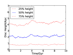
Figure 3: The evolution of the quarter-mass, half-mass and three-quarter-mass heights of the disc in a spherical NFW profile, evolved for 10 Gyrs. The vertical height of the disc remains unchanged, validating our way of setting up initial conditions.

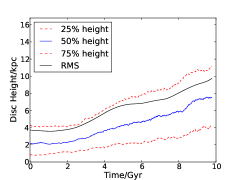
(a) Model 3

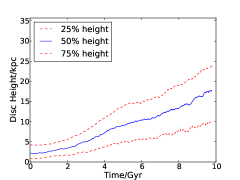
(b) Model 4

Figure 4: Scale height evolution of the disc of satellites in an oblate NFW profile tilted at 77.5^∘ (upper panel). This means that the principal axes of the halo are aligned with the stellar disc of M31. The full black line shows the evolution of the rms scatter, which is the quantity measured by observers. It typically lies between the half-mass and three-quarter-mass scaleheights. Also shown is a model in which the disc of satellites is tilted at 45.0^∘ to the halo (lower panel). In both cases, the thin disc becomes fat over timescales $\sim 6$ Gyr. This is a general result whenever the disc of satellites is misaligned with the principal planes.

3 The Disc of Satellites

3.1 Initial Conditions

The satellite galaxies lie in the near-Keplerian outer parts of the M31 halo. We first develop a way of setting up approximate initial conditions for thin discs in the outer parts of a triaxial halo.

First, Keplerian semi-major axes $a$ and eccentricities $e$ are drawn from uniform distributions of 100-200 kpc and 0.0-0.5 respectively, with a random line of apsides ${\theta_{\rm a}}$ in the disc ($x,y$) plane. This gives the Cartesian coordinates at apocentre as

$$\Bigl{(}x_{\rm a},y_{\rm a}\Bigr{)}=a(1+e)\Bigl{(}\cos{\theta_{\rm a}},\sin{\theta_{\rm a}}\Bigr{)},$$ (17)

A Keplerian ellipse has a tangential velocity at apocentre of

$$v_{\phi}=\sqrt{\frac{GM(1-e)}{a(1+e)}},$$ (18)

giving planar velocities of

$$\Bigl{(}v_{x},v_{y}\Bigr{)}=\frac{v_{\phi}}{a(1+e)}\Bigl{(}y_{\rm a},-x_{\rm a}\Bigr{)}.$$ (19)

So far, the disc is razor-thin. To thicken up the disc, orbital inclinations $i$ are chosen uniformly in the range 0-3^∘. The vertical motion at apocentre in a near-Keplerian potential can then be approximated to first order as

$$\ddot{z}=\frac{-GMz}{r^{3}}=\omega^{2}_{z}z,\qquad\omega_{z}=\sqrt{\frac{GM}{a^{3}(1+e)^{3}}}.$$ (20)

This allows us to choose a random phase, $\phi$ from 0 to $2\pi$, such that

$$z_{\rm a}=a(1+e)\sin i\cos{\phi},\qquad v_{z}=a(1+e)\omega_{z}\sin i\sin{\phi}.$$ (21)

This completes the specification of the apocentres of our orbits. Of course, we wish our satellites to begin at a random point along their orbits. The Keplerian orbital period is $P=\sqrt{4\pi^{2}a^{3}/(GM)}$. A random number is generated in the range 0 to $P$, and the orbit evolved forward for this time from apocentre. The properties of the satellite at this time provide the initial phase-space coordinates at the start of our simulations

A disc created in this fashion is extended and thin. Fig. 3 shows the evolution of such a disc in a spherical Navarro-Frenk-White potential. It starts out with an rms vertical scatter of $3.7$ kpc, and the coloured lines show the evolution of scaleheights enclosing a quarter, a half and three-quarters of the satellites. For a disc with a vertical Gaussian profile, the half-mass thickness is comparable to the rms scatter. After 10 Gyr, the disc has a vertical scatter of $4.5$ kpc, only slightly increased from its starting value. It is much thinner than that claimed for the disc of satellites around M31 (Ibata et al., 2013). This confirms the stability of the disc and validates our algorithm for initial conditions.

3.2 The Tidal Effects of the Milky Way Galaxy

Finally, we include the effect of tidal forces from the Milky Way galaxy on the disc of satellites. The present day separation of the Milky Way and M31 is $\sim 770$ kpc, with the Milky Way approximately coplanar with the observed disc around M31. As this distance was still greater in the recent past, the Milky Way galaxy does not need to be modelled in detail in our simulations. Accordingly, the Milky Way halo is taken as a spherical NFW profile with a halo mass $M$ of $10^{12}M_{\odot}$ and a concentration $c$ of $10$. The evolution of the separation between the Milky Way and M31 can be modelled with the Timing Argument (Peebles, 1993), which assumes that the mutual gravitation of the two galaxies caused them to decouple from the Hubble flow at high redshift. Specifically, we use eqn (10) in van der Marel & Guhathakurta (2008), with our simulations running from t = 3.95 Gyr to the present day at t = 13.73 Gyr.

3.3 Results

We performed orbit integrations for a population of 1000 satellite galaxies modelled as test particles in a variety of oblate, prolate and triaxial haloes listed in Table 1.

To study the vertical structure, we track the evolution of the quarter-mass, half-mass and three-quarter-mass heights over 10 Gyr. If the disc thickens, then the growth of the disc half-mass height with time is fitted to an exponential functional form, $z=z_{0}\exp t/{t_{\rm h}}$, and the $e$-folding timescale ${t_{\rm h}}$ is reported in Table 1.

The first two models record simulation results for oblate and prolate E2 haloes. The disc of satellites lies either in the polar (model 1) or equatorial planes (model 2). The tidal effects of the Milky Way are incorporated, as well as of course the torques from the asphericity of the haloes. However, these forces do not disturb the serenity of the discs, which are long-lived. This result is straightforward to understand. Circular orbits in the equatorial plane of either oblate or prolate dark haloes are stable, and can sire families of orbits which are long-lived and populate a disc of satellites. Equally, the non-circular, but closed and periodic, orbits in the meridional planes of either oblate or prolate haloes can be used to build stable discs.

However, any misalignment of the principal planes of the oblate or prolate halo with the disc of satellites causes the disc to fatten. This is the case in models 3 and 4 in Table 1. The upper panel of Fig. 4 shows an E2 oblate halo, in which the equatorial plane is now aligned with the stellar disc of the M31 galaxy, which is at an inclination of $77.5^{\circ}$(see e.g., Hodge, 1992). The disc of satellites no longer lies in the equatorial plane. This is a natural model to use if we believe that the shape of the dark matter halo does not twist or misalign with increasing radius. Notice that the disc of satellites is now no longer a stable structure – the disc height doubles within $\sim 7$ Gyr. In a flattened halo, the only planar orbits are confined to the principal planes. Once the halo is misaligned with the disc of satellites, then torques from the quadrupole and higher moments cause the disc to thicken. The bottom panel of Fig. 4 again shows an E2 oblate halo, but the misalignment is now $45^{\circ}$. This dark halo is misaligned both with the stellar disc and the disc of satellites. The disc is fattened more quickly, with a doubling of the disc height in $\sim 5.5$ Gyr. At the end of the simulations, the rms scatter is $\sim 19$ kpc, comparable to the rms scatter claimed for the disc of satellites.

Models 5 and 6 of Table 1 show the effects of incorporating triaxiality. In model 5, the halo is aligned so that the $x$ axis points to the Milky Way and the disc of satellites occupies the ($x,y$) plane. As noted in our discussion of closed orbits, stable closed orbits can exist in the planes perpendicular to the long and the short axes of a triaxial halo. The simulation demonstrates that the disc can survive unthickened for timescales $\sim 10$ Gyr. Once however, the halo is misaligned with the disc of satellites, thickening does occur. For example, even the modest misalignment of $12.5^{\circ}$ of model 6 gives a doubling of the disc height on a timescale of $\sim 7$ Gyr.

4 Conclusions

We have presented a simple triaxial generalization of the Navarro-Frenk-White model. It has an elementary potential-density pair. The parameters of the model can be chosen to lie on the cosmological mass-concentration relation, and tuned to give any desired axis ratios at large and small radii. So, it is easy to build cosmologically-inspired haloes with radially varying triaxiality, tailored for any purpose – for example, oblate in the centre but prolate in the outer parts, or triaxial in the centre and round in the outer parts.

We have used the haloes to examine the longevity of a vast, thin disc of satellites. This is motivated by the observational claims of Ibata et al. (2013), who have surveyed the outer parts of M31. Such a disc is in general not long-lived, and thickens due to torques and tidal forces. The disc of satellites therefore provides a powerful constraint on the shape and orientation of the M31 dark halo. We find that there are the following three possibilities for a long-lived disc:

[1] If the M31 dark halo is spherical, then a thin disc of satellites can survive for timescales of the order of 10 Gyr.

[2] If the M31 dark halo is oblate or prolate, and the disc of satellites lies in the equatorial or polar plane of the spheroidal potential, then it is also thin and long-lived. The same holds true for triaxial haloes, provided the disc lies in the plane perpendicular to the long or short axis. For M31, such a configuration would require that the principal axes of the dark halo at large radii are misaligned with the axes of the stellar disc of the galaxy itself. This requires the M31 potential to twist on moving outwards from the baryon-dominated central parts to the outer halo. Such misalignment is often observed in numerical simulations (see e.g., Deason et al., 2011).

[3] For all other orientations, the disc of satellites must thicken and its vertical height grows exponentially with an e-folding time of $\sim 5$-$7$ Gyr. If its present rms scatter is $\sim 12$ kpc, then it must have been formed with a scaleheight that is astonishingly thin, perhaps only $2$ or $3$ kpc despite being hundreds of kpc across. This seems implausible. Nonetheless, the problem could be ameliorated if there are more satellites associated with the disc of satellites than suggested by (Ibata et al., 2013), and so its present-day thickness could be greater.

References

- Allgood et al. (2006) Allgood, B., Flores, R. A., Primack, J. R., et al. 2006, MNRAS, 367, 1781
- Conn et al. (2012) Conn, A.R., et al., 2012, ApJ, 758, 11
- Conn et al. (2013) Conn, A.R., et al., 2013, ApJ, 766 120
- Deason et al. (2011) Deason, A.J., McCarthy, I.G., Font, A.S., et al. 2011, MNRAS, 415, 2607
- de Zeeuw & Carollo (1996) de Zeeuw, P.T., Carollo, C.M., 1996, MNRAS, 281, 1333
- Dubinski (1994) Dubinski, J. 1994, ApJ, 431, 617
- Fusi Pecci et al. (1995) Fusi Pecci, F., Bellazinni, M., Cacciair, C., Ferraro, F.R., 1995, AJ, 110, 1664
- Gerhard & Vietri (1986) Gerhard, O.E., Vietri, M., 1986, MNRAS, 223, 377
- Heiligman & Schwarzschild (1979) Heiligman, G., Schwarzschild, M. 1979, ApJ, 233, 872
- Hernquist & Quinn (1989) Hernquist, L., Quinn, P.J., 1989, ApJ, 342, 1
- Hodge (1992) Hodge, P.W. 1992 The Andromeda Galaxy, Kluwer, Dordrecht
- Ibata et al. (2013) Ibata, R.A., Lewis, G.F., Conn, A.R., et al. 2013, Nat, 493, 62
- Jing & Suto (2002) Jing, Y. P., Suto, Y. 2002, ApJ, 574, 538
- Koch & Grebel (2006) Koch, A., Grebel E., 2006, AJ, 1405
- Kazantzidis et al. (2004) Kazantzidis, S., Kravtsov, A. V., Zentner, A. R., et al. 2004, ApJ, 611, L73
- Maccio et al. (2007) Maccio, A.V., Dutton A.A., van den Bosch, F., Moore, B., Potter, D., Stadel J., 2007, MNRAS, 378, 55
- Mo, van den Bosch & White (2010) Mo, H.J., van den Bosch, F., White, S., 2010, Galaxy Formation and Evolution, Cambridge University press, Cambridge, chap. 7
- Peebles (1993) Peebles, P.J.E., 1993, Principles of Physical Cosmology, Princeton University Press, Princeton
- Schwarzschild (1979) Schwarzschild, M. 1979, ApJ, 232, 236
- Schwarzschild (1993) Schwarzschild, M. 1993, ApJ, 409, 563
- van der Marel & Guhathakurta (2008) van der Marel, R. P., Guhathakurta, P. 2008, ApJ, 678, 187
- Zemp et al. (2012) Zemp, M., Gnedin, O. Y., Gnedin, N. Y., & Kravtsov, A. V. 2012, ApJ, 748, 54