Integral Equations for Computing AC Losses of Radially and Polygonally Arranged HTS Thin Tapes

Abstract

In this paper we derive the integral equations for radially and polygonally arranged high-temperature superconductor thin tapes and we solve them by finite-element method. The superconductor is modeled with a non-linear power law, which allows the possibility of considering the dependence of the parameters on the magnetic field or the position. The ac losses are computed for a variety of geometrical configurations and for various values of the transport current. Differences with respect to existing analytical models, which are developed in the framework of the critical state model and only for certain values of the transport current, are pointed out.

I Introduction

The current density distribution and the ac losses of thin superconductors carrying ac current and/or subjected to external ac magnetic field can be calculated by solving the integral equations for the current density distribution by means of finite elements [1]. The integral equation (IE) model was first proposed in [1] for individual tapes; then, it was extended to the case of interacting tapes in [2], where the electromagnetic interaction between tapes was calculated by means of an auxiliary 2-D magnetostatic model; finally, it was developed to the stage where the interaction between tapes is directly included in the integral equation to be solved [3].

The most important advantages of this approach, especially compared to analytical formulations, are that arbitrary current-voltage characteristics for the superconductor and the dependence of the superconductors parameters (e.g. the critical current density $J_{c}$) on the position and the local magnetic field can be easily incorporated.

The IE model has been successfully used to compute the ac losses of interacting tapes and a very good agreement with experimental data has been found for tapes characterized by a lateral variation of $J_{c}$ [4] and arranged in a bifilar winding for fault-current limiter application [5].

In this paper we use the approach utilized in [3] to derive and solve the integral equations for the current density distribution in two other cases of practical interest, namely cables with radially and polygonally arranged thin superconducting tapes. The former is potentially interesting for bus bar applications (especially with bidirectional currents, see [6, 7]); the latter can be useful to quickly estimate the losses of straight cable samples [8]. These configurations were analyzed by Mawatari and Kajikawa under the assumptions of the critical state model [9, 10]. Their method is not devoid of elegance, however their solutions are valid only for certain current levels ($I\ll I_{c}$ for both configurations and $I=I_{c}$ for the polygonal configuration only), which are usually not found in practical applications. On the contrary, the IE approach allows using arbitrary current levels. In addition, it can take the dependence of certain parameters on the local magnetic field and/or on the position inside the tape into account, see for example [4] and [11]. This latter dependence is very important for simulating real ReBCO coated conductors, which often present a reduced $J_{c}$ near the edges due to the manufacturing process [12, 13].

The paper is organized as follows. Section II describes in detail the derivation of the integral equations for the cases under scrutiny. Section III contains the main results of our investigation: we discuss the dependence of the ac losses on the geometrical parameters and we show the obtained current profiles; differences from and analogies with the analytical models are pointed out. Finally, section IV draws the main conclusions.

II Derivation of the integral equations

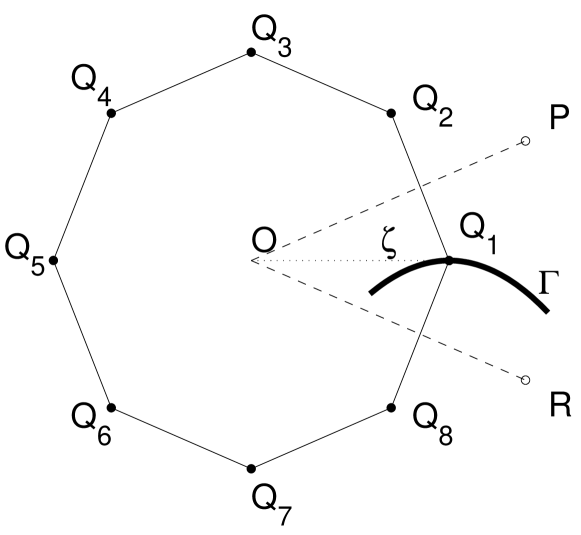
Figure 1: Reference periodical geometry used for the derivation of the integral equations – see section II.

In the complex plane, we consider the vertices $Q_{i}$ of a regular polygon with $n$ sides centered in the origin $O$ and a point $P$ as shown in Fig. 1. If we call $z$ the point $P$ and $\zeta$ the point $Q_{1}$, the vertices of the polygon will be given by $Q_{k}=\omega_{k-1}\zeta$, where $\omega_{k}=\exp(2\pi ik/n)$ are the $n$-th roots of the unity. Based on the properties of those roots, we shall have

$$\prod_{k=0}^{n-1}(z-\omega_{k}\zeta)=z^{n}-\zeta^{n}.$$ (1)

Taking the logarithm of both members, we have

$$\sum_{k=0}^{n-1}\log(z-\omega_{k}\zeta)=\log(z^{n}-\zeta^{n})$$ (2)

and by deriving with respect to $z$ we obtain the identity

$$\sum_{k=0}^{n-1}\frac{1}{z-\omega_{k}\zeta}=\frac{nz^{n-1}}{z^{n}-\zeta^{n}}.$$ (3)

II-A Magnetic field generated by current lines arranged with angular periodicity

Since in two-dimensions the Biot-Savart law for the magnetic field generated by a current line $I_{0}$ situated in $\zeta$ can be expressed in the complex plane by the following complex expression

$$H(z)=H_{y}(z)+iH_{x}(z)=\frac{I_{0}}{2\pi}\frac{1}{z-\zeta},$$ (4)

we shall have that, according to (3), the magnetic field generated by $n$ identical current lines situated in the vertices $\omega_{k}\zeta$ of a regular polygon of radius $\zeta$ is

$$H(z)=\frac{I_{0}}{2\pi}\sum_{k=0}^{n-1}\frac{1}{z-\omega_{k}\zeta}=\frac{I_{0}}{2\pi}\frac{nz^{n-1}}{z^{n}-\zeta^{n}}.$$ (5)

In the case where $n=2m$ and the currents have alternate signs, we can write

$$H(z) =\frac{I_{0}}{2\pi}\sum_{k=0}^{n-1}\frac{(-1)^{k}}{z-\omega_{k}\zeta}$$

$$=\frac{I_{0}}{2\pi}\left(\sum_{k=0}^{m-1}\frac{1}{z-\omega_{2k}\zeta}-\sum_{k=0}^{m-1}\frac{1}{z-\omega_{2k+1}\zeta}\right)$$

$$=\frac{I_{0}}{2\pi}\left(\sum_{k=0}^{m-1}\frac{1}{z-\omega_{2k}\zeta}-\sum_{k=0}^{m-1}\frac{1}{z-\omega_{2k}(\omega_{1}\zeta)}\right).$$ (6)

Using (3) and the fact that $\omega_{1}^{m}=\omega_{1}^{n/2}=\exp(i\pi)=-1$, for $m$ currents we can write

$$H(z) =\frac{I_{0}}{2\pi}\left(\frac{mz^{m-1}}{z^{m}-\zeta^{m}}-\frac{mz^{m-1}}{z^{m}-\omega_{1}^{m}\zeta^{m}}\right)$$

$$=\frac{I_{0}}{2\pi}\left(\frac{mz^{m-1}}{z^{m}-\zeta^{m}}-\frac{mz^{m-1}}{z^{m}+\zeta^{m}}\right)=\frac{I_{0}}{2\pi}\frac{nz^{n/2-1}\zeta^{n/2}}{z^{n}-\zeta^{n}}.$$ (7)

II-B Magnetic field generated by current line distributions arranged with angular periodicity

Let us consider the case where the magnetic field is generated by a distribution of current lines $J(z)$ along a path $\Gamma$ with angular periodicity, as shown in Fig. 1. The magnetic field is obtained simply by integrating (5) or (II-A) along $\Gamma$

$$H(z)=\frac{1}{{2\pi}}\int\limits_{\Gamma}{J(\zeta)\frac{{n\,{z^{n-1}}}}{{{z^{n}}-{\zeta^{n}}}}\,d\zeta}.$$ (8)

Due to the angular periodicity it is sufficient to study the magnetic field in the angular sector $\alpha=2\pi/n$. We will now study two cases interesting for practical applications: a system of $n$ tapes with radial and polygonal arrangement, which are schematically represented in Fig. 2.

II-C System of $n$ radially arranged tapes

Let us place the tape along a segment $(b,a)$ on the $x$-axis with a current density distribution $J(x)$ – see Fig. 2. The magnetic field will be given by the integral

$$H(x)=\frac{1}{{2\pi}}\int\limits_{b}^{a}{J(\xi)\frac{{n\,{x^{n-1}}}}{{{x^{n}}-{\xi^{n}}}}\,d\xi}.$$ (9)

We can compute the flux (in each tape) between the edge $b$ and an arbitrary point $x<a$ as

$$\Phi(x) =\int\limits_{b}^{x}{{H_{y}}(t)dt}={\mathop{\rm Re}\nolimits}\int\limits_{b}^{x}{H(t)dt}$$

$$=\frac{1}{{2\pi}}\int\limits_{b}^{x}{dt}\int\limits_{b}^{a}{J(\xi)\frac{{n\,{t^{n-1}}}}{{{t^{n}}-{\xi^{n}}}}\,d\xi}$$

$$=\frac{1}{{2\pi}}\int\limits_{b}^{a}{J(\xi)\,d\xi\int\limits_{b}^{x}{\frac{{n\,{t^{n-1}}}}{{{t^{n}}-{\xi^{n}}}}\,}dt}$$

$$=\frac{1}{{2\pi}}\int\limits_{b}^{a}{J(\xi)}\,\ln\left|{\frac{{{x^{n}}-{\xi^{n}}}}{{{b^{n}}-{\xi^{n}}}}}\right|\,d\xi.$$ (10)

Similarly to what was done in [1], using this expression for the flux we can define the integral equation for the computation of the current density

$$\rho J(x,t)=\mu d\frac{1}{{2\pi}}\int\limits_{-a}^{a}{\dot{J}(\xi,t)\ln\left|{{x^{n}}-{\xi^{n}}}\right|}\,d\xi+C(t),$$ (11)

where the term $C(t)$ is the contribution to the integral in (II-C) due to the logarithmic part not dependent on the flux variable $x$. In practice the $C(t)$ term is obtained by imposing the total current $I(t)$ flowing in each tape. For the solution of the integral equation by finite elements the term does not need to be explicitly introduced in the equation, since it is automatically evaluated by means of the integral constraint.

$$\int\limits_{-a}^{a}J(x,t)\,dx=I(t).$$ (12)

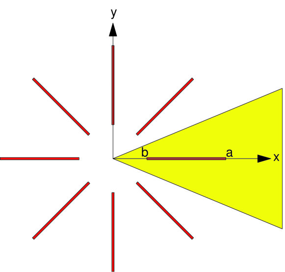
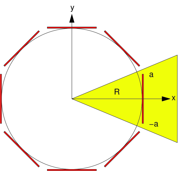
Figure 2: Schematic drawings of the geometries considered in this work: (a) Radially-arranged and (b) polygonally-arranged superconducting thin tapes. For the radial arrangement, both unidirectional and bidirectional currents are considered.

In case of bidirectional currents (neighboring tapes carrying current of the same amplitude but with opposite direction), one can follow the same procedure to find the integral equation for the current density

$$\rho J(x,t)=\mu d\frac{1}{{2\pi}}\int\limits_{-a}^{a}{\dot{J}(\xi,t)\ln\left|{\frac{{{x^{m}}-{\xi^{m}}}}{{{x^{m}}+{\xi^{m}}}}}\right|}\,d\xi+C(t).$$ (13)

II-D System of $n$ polygonally arranged tapes

In this case the tape can be represented by the segment $(-a,a)$ at a distance $R$ from the origin – see Fig. 2. Obviously, in order to avoid tape overlapping, the condition $R>a\cot(\pi/n)$ must hold. According to (8) the magnetic field is given by the integral

$$H(z)=\frac{1}{{2\pi}}\int\limits_{-a}^{a}{J(\eta)\frac{{n\,{z^{n-1}}}}{{{z^{n}}-{{(R+i\eta)}^{n}}}}\,d\eta}.$$ (14)

With this formula we can compute the flux (in each tape) between the edge $-a$ and an arbitrary point $y<a$ as

$$\Phi(y) =\int\limits_{-a}^{y}{{H_{x}}(t)dt}={\mathop{\rm Im}\nolimits}\int\limits_{-a}^{y}{H(t)dt}$$

$$=-\frac{1}{{2\pi}}\int\limits_{-a}^{y}{dt}\int\limits_{-a}^{a}{J(\eta)\frac{{n\,{{(R+it)}^{n-1}}}}{{{{(R+it)}^{n}}-{{(R+i\eta)}^{n}}}}\,d\eta}$$

$$=-\frac{1}{{2\pi}}\int\limits_{-a}^{a}{J(\eta)\,d\eta\,\int\limits_{-a}^{y}{\frac{{n\,{{(R+it)}^{n-1}}}}{{{{(R+it)}^{n}}-{{(R+i\eta)}^{n}}}}\,}dt}$$

$$=-\frac{1}{{2\pi}}\int\limits_{-a}^{a}{J(\eta)}\,\ln\left|{\frac{{{{(R+iy)}^{n}}-{{(R+i\eta)}^{n}}}}{{{{(R+ia)}^{n}}-{{(R+i\eta)}^{n}}}}}\right|\,d\eta.$$ (15)

From this expression we can derive the integral equation for the current density

$$\rho J(y,t)=\mu d\frac{1}{{2\pi}}\int\limits_{-a}^{a}{\dot{J}(\eta,t)\ln\left|{{{(R+iy)}^{n}}-{{(R+i\eta)}^{n}}}\right|}\,d\eta+C(t).$$ (16)

III Results

In this section we show the ac loss numerical results for various configurations, including a comparison with those obtained with the analytical models [9, 10]. The plotted ac loss values represent the losses per tape, normalized by the loss value of a single isolated tape carrying the same transport current: it is therefore what we called a geometric factor, representing the change of the ac loss value with respect to that of a single isolated tape, due to the particular geometric configuration under scrutiny.

For our simulations, we considered a tape 12 mm wide with $I_{c}=330$ A and $n=35$, representative of state-of-the-art YBCO coated conductors. The frequency of the current source was 50 Hz.

For validation purpose, we compared the current density profiles with those obtained by means of the 2-D FEM model developed in [14], always obtaining an excellent agreement – an example is shown later in this section.

Figure 3 shows the geometric factor of the cable with radially arranged tapes carrying current in the same direction as a function of the distance of the tapes from the center of the cable – see Fig. 2 for reference. This is not a convenient geometry from the point of view of ac losses because each tape undergoes the magnetic field generated by the neighbors. At the tape’s edge the field contributions sum up, which results in losses that are always higher than those of a single isolated tape. The higher the number of tapes in the cable, the higher the losses. Plotted with a continuous line is the loss value predicted with the analytical model [9], which was developed only for the case $I\ll I_{c}$. It can be noticed that for the case $I=0.1I_{c}$ the results of the IE model agree well with the analytical predictions, whereas for higher current values they are significantly different. The difference increases with the number of tapes in the cable.

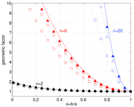
Figure 3: Geometric factor indicating the ac losses of a single tape in the radial configuration with unidirectional current with respect to the ac losses of an individual tape carrying the same current. The losses are plotted as a function of the ratio $b/a$ – see Fig. 2 for reference. Results are shown for a different number of tapes (2, 6, 20) and for different current values: $I/I_{c}=0.1$ (triangles), 0.5 (squares) and 0.9 (circles). The continuous line represents the geometric factor calculated by equation (20) in [9].

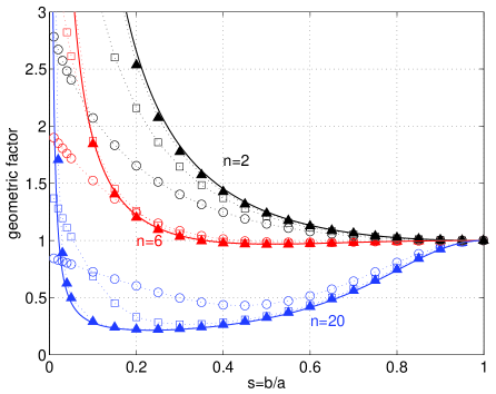
Figure 4: Geometric factor indicating the ac losses of a single tape in the radial configuration with bidirectional current with respect to the ac losses of an individual tape carrying the same current. The losses are plotted as a function of the ratio $b/a$ – see Fig. 2 for reference. Results are shown for a different number of tapes (2, 6, 20) and for different current values: $I/I_{c}=0.1$ (triangles), 0.5 (squares) and 0.9 (circles). The continuous line represents the geometric factor calculated by equation (25) in [9].

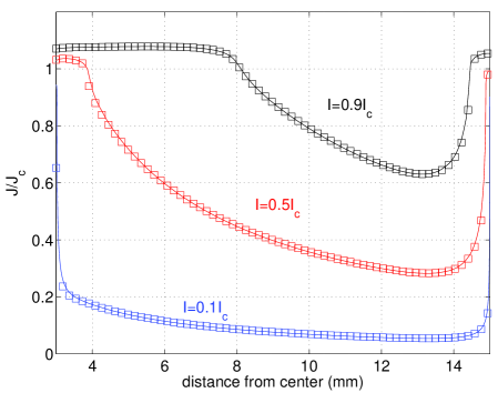
Figure 5: Current density profiles in the radially arranged tape configuration for $s=0.2$ ($b=3$ mm, $a=15$ mm) and $n$=20 for different values of the transport current. The profiles are taken at the peak instant of the transport current. The current density is normalized with respect to the critical value $J_{c}$. For validation purpose, the profiles are calculated with the integral equation model (continuous lines) and with the 2-D FEM model developed in [14] (symbols).

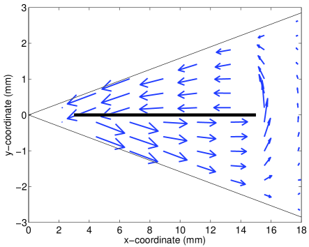
Figure 6: Magnetic field generated by a tape in the radial configuration in the case of bidirectional currents: the magnetic field is tangential to the boundaries and the normal component vanishes there. In the case of unidirectional currents, the opposite happens. The represented case corresponds to $n=20$, $b=3$ mm, $a=15$ mm. Different scales are used for the two axes.

Figure 4 shows the same type of results as Fig. 3, but for bidirectional currents, i.e. adjacent tapes carry the same current but with opposite direction. This is a more advantageous configuration from the point of view of ac losses, because in certain cases the losses are significantly lower than those of a single isolated tape. More specifically this happens for a sufficiently high number of tapes. This is due to the fact that, similarly to the case of bifilar coils [15], the perpendicular component of the magnetic field at the tape’s edge is significantly reduced. However, the distance of the tapes from the center also plays an important role and if the tapes are situated very close to the center of the cable ($s\rightarrow 0$) the loss reduction vanishes, especially at high currents. Also for this configuration we found a good agreement between the IE model and the analytical predictions in the case $I=0.1I_{c}$ and substantial differences in the case of higher currents.

Figure 5 shows the current density profiles for $s=0.2$ ($b=3$ mm, $a=15$ mm) for different values of the transport current. The shape of the profile drastically changes with the current amplitude, and one can clearly see that only for very low currents the Meissner-state approach described in [9] holds. In the figure, results obtained with the 2-D FEM model developed in [14] are also shown (symbols). The overlapping of the profiles computed with the two models is perfect. Due to periodicity, in the 2-D model one needs to simulate only one sector. The condition of uni- or bi-directional currents is obtained by appropriately setting the boundary conditions for the magnetic field (state variable) on the domain’s boundary, see also Fig. 6. In the case of uni-directional currents, the tangential component of the magnetic field vanishes on the simulated boundary; conversely, in the case of bi-directional currents, the normal component vanishes (as shown in the figure).

Figure 7 shows the geometric factor of the losses for a polygonal cable. Losses are plotted as a function of $a/R\cot(\pi/n)$, and in the low current limit they are in excellent agreement with the results of the analytical model in [10]. The agreement with the analytical model is not as perfect in the case $I=I_{c}$. This is most probably due to the intrinsic difference between the superconductor’s characteristics in the two models: with the critical state model (used in the analytical formulas) the tape is filled with current at $I=I_{c}$ and $J=J_{c}$ everywhere; on the contrary, with the power-law resistivity (used in the IE model), current density values higher than $J_{c}$ are allowed and the $J$ is not just constant everywhere.

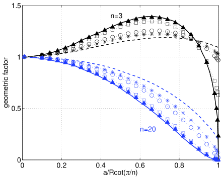
Figure 7: Geometric factor indicating the ac losses of a single tape in the polygonal configuration with respect to the ac losses of an individual tape carrying the same current. The losses are plotted as a function of $a/R\cot(\pi/n)$. The continuous and dashed lines indicate the analytical predictions for $I\ll I_{c}$ and $I=I_{c}$ from [10], respectively.

IV Conclusions

We derived the integral equations for radially and polygonally arranged thin HTS tapes and solved them by finite elements. The obtained results are in good agreement with existing analytical model, which are valid only for certain values of the transport current. Our integral equation model, on the contrary, can consider arbitrary values of the transport current. Another important advantage of the IE model is that the dependence of the critical current on the lateral position inside the tape or on the local magnetic field can be easily implemented. In addition, since only one tape is simulated in 1-D, the solution takes only few seconds; the IE model can therefore be used to simulate a large number of configurations for design optimization purposes.

Finally, we would like to conclude with a practical remark. Similarly to the cases presented in [3], the magnetic interaction between the tapes in integral equations (11), (13), (16) is expressed by a term $K(x,t)=\int_{-a}^{a}k(x-\xi)\dot{J}(\xi){\rm d}\xi$, i.e. by the finite space convolution of the time derivative of the sheet current $J(x,t)$ with a kernel $k(x)$ of logarithmic type. This kernel is the only thing that need to be changed to study the different geometries. This means that one needs to build only one file in the finite element program and simply change the selection of the kernel to simulate different configurations.

References

- [1] R. Brambilla, F. Grilli, L. Martini, and F. Sirois, “Integral equations for the current density in thin conductors and their solution by finite-element method,” Superconductor Science and Technology, vol. 21, no. 10, p. 105008, 2008.
- [2] F. Grilli, R. Brambilla, L. Martini, F. Sirois, D. N. Nguyen, and S. P. Ashworth, “Current Density Distribution in Multiple YBCO Coated Conductors by Coupled Integral Equations,” IEEE Transactions on Applied Superconductivity, vol. 19, no. 3, pp. 2859–2862, 2009.
- [3] R. Brambilla, F. Grilli, D. N. Nguyen, L. Martini, and F. Sirois, “AC losses in thin superconductors: the integral equation method applied to stacks and windings,” Superconductor Science and Technology, vol. 22, no. 7, p. 075018, 2009.
- [4] D. N. Nguyen, F. Grilli, S. P. Ashworth, and J. O. Willis, “Ac loss study of antiparallel connected YBCO coated conductors,” Superconductor Science and Technology, vol. 22, no. 5, p. 055014, 2009.
- [5] S. Elschner, A. Kudymow, J. Brand, S. Fink, W. Goldacker, F. Grilli, M. Noe, M. Vojenciak, A. Hobl, M. Bludau, C. Jänke, S. Krämer, and J. Bock, “ENSYSTROB – Design, manufacturing and test of a 3-phase resistive fault current limiter based on coated conductors for medium voltage application,” Physica C, 2012. Submitted.
- [6] T. Kato, N. Shibuta, K. Sato, T. Isono, T. Ando, and H. Tsuji, “Development of a 1kA-Class Go and Return High- Superconducting Bus Bar,” Proceedngs of the Fifth International Symposium on Superconductivity, pp. 1243–1246, 1993.
- [7] T. Ando, T. Isono, H. Tsuji, T. Kato, T. Hikata, and K. Sat0, “Development of a 10kA-class High-Tc Superconducting Bus Bar,” IEEE Transactions on Applied Superconductivity, vol. 5, no. 2, pp. 817–820, 1995.
- [8] N. Amemiya, Z. Jiang, M. Nakahata, M. Yagi, S. Mukoyama, N. Kashima, S. Nagaya, and Y. Shiohara, “AC Loss Reduction of Superconducting Power Transmission Cables Composed of Coated Conductors,” IEEE Transactions on Applied Superconductivity, vol. 17, no. 2, pp. 1712–1717, 2007.
- [9] Y. Mawatari and K. Kajikawa, “Alternating current loss in radially arranged superconducting strips,” Applied Physics Letters, vol. 88, p. 092503, 2006.
- [10] ——, “Hysteretic ac loss of polygonally arranged superconducting strips carrying ac transport current,” Applied Physics Letters, vol. 92, p. 012504, 2008.
- [11] F. Grilli, F. Sirois, S. Brault, R. Brambilla, L. Martini, D. N. Nguyen, and W. Goldacker, “Edge and top/bottom losses in non-inductive coated conductor coils with small separation between tapes,” Superconductor Science and Technology, vol. 23, p. 034017, 2010.
- [12] N. Amemiya, O. Maruyama, M. Mori, N. Kashima, T. Watanabe, S. Nagaya, and Y. Shiohara, “Lateral distribution of YBCO coated conductors fabricated by IBAD/MOCVD process,” Physica C, vol. 445-448, pp. 712–716, 2006.
- [13] J. Hänisch, F. M. Mueller, S. Ashworth, J. Y. Coulter, and V. Matias, “Measurement of the transverse profiles of coated conductors using a magnetic knife of permanent magnets,” Superconductor Science and Technology, vol. 21, p. 115021, 2008.
- [14] R. Brambilla, F. Grilli, and L. Martini, “Development of an edge-element model for AC loss computation of high-temperature superconductors,” Superconductor Science and Technology, vol. 20, no. 1, pp. 16–24, 2007.
- [15] J. R. Clem, “Field and current distributions and ac losses in a bifilar stack of superconducting strips,” Physical Review B, vol. 77, p. 134506, 2008.