DNA Reservoir Computing:
A Novel Molecular Computing Approach

Abstract

We propose a novel molecular computing approach based on reservoir computing. In reservoir computing, a dynamical core, called a reservoir, is perturbed with an external input signal while a readout layer maps the reservoir dynamics to a target output. Computation takes place as a transformation from the input space to a high-dimensional spatiotemporal feature space created by the transient dynamics of the reservoir. The readout layer then combines these features to produce the target output. We show that coupled deoxyribozyme oscillators can act as the reservoir. We show that despite using only three coupled oscillators, a molecular reservoir computer could achieve $90\%$ accuracy on a benchmark temporal problem.

1 Introduction

A reservoir computer is a device that uses transient dynamics of a system in a critical regime—a regime in which perturbations to the system’s trajectory in its phase space neither spread nor die out—to transform an input signal into a desired output [1]. We propose a novel technique for molecular computing based on the dynamics of molecular reactions in a microfluidic setting. The dynamical core of the system that contains the molecular reaction is called a reservoir. We design a simple in-silico reservoir computer using a network of deoxyribozyme oscillators [2], and use it to solve temporal tasks. The advantage of this method is that it does not require any specific structure for the reservoir implementation except for rich dynamics. This makes the method an attractive approach to be used with emerging computing architectures [3].

We choose deoxyribozyme oscillators due to the simplicity of the corresponding mathematical model and the rich dynamics that it produces. In principle, the design is generalizable to any set of reactions that show rich dynamics. We reduce the oscillator model in [2] to a form more amenable to mathematical analysis. Using the reduced model, we show that the oscillator dynamics can be easily tuned to our needs. The model describes the oscillatory dynamics of three product and three substrate species in a network of three coupled oscillators. We introduce the input to the oscillator network by fluctuating the supply of substrate molecules and we train a readout layer to map the oscillator dynamics onto a target output. For a complete physical reservoir computing design, two main problems should be addressed: (1) physical implementation of the reservoir and (2) physical implementation of the readout layer. In this paper, we focus on a chemical design for the reservoir and assume that the oscillator dynamics can be read using fluorescent probes and processed using software. We aim to design a complete chemical implementation of the reservoir and the readout layer in a future work (cf. Section 5). A similar path was taken by Smerieri et al. [4] to achieve an all-analog reservoir computing design using an optical reservoir introduced by Paquot et al. [5].

We use the molecular reservoir computer to solve two temporal tasks of different levels of difficulty. For both tasks, the readout layer must compute a function of past inputs to the reservoir. For Task A, the output is a function of two immediate past inputs, and for Task B, the output is a function of two past inputs, one $\tau$ seconds ago and the other $\frac{3}{2}\tau$ seconds ago. We implement two varieties of reservoir computer, one in which the readout layer only reads the dynamics of product concentrations and another in which both product and substrate concentrations are read. We show that the product-only version achieves about $70\%$ accuracy on Task A and about $80\%$ accuracy on Task B, whereas the product-and-substrate version achieves about $80\%$ accuracy on Task A and $90\%$ accuracy on Task B. The higher performance on Task B is due to the longer time delay, which gives the reservoir enough time to process the input. Compared with other reservoir computer implementations, the molecular reservoir computer performance is surprisingly good despite the reservoir being made of only three coupled oscillators.

2 Reservoir Computing

As reservoir computing (RC) is a relatively new paradigm, we try to convey the sense of how it computes and explain why it is suitable for molecular computing. RC achieves computation using the dynamics of an excitable medium, the reservoir [6]. We perturb the intrinsic dynamics of the reservoir using a time-varying input and then read and translate the traces of the perturbation on the system’s trajectory onto a target output.

RC was developed independently by Maass et al. [7] as a model of information processing in cortical microcircuits, and by Jaeger [8] as an alternative approach to time-series analysis using Recurrent Neural Networks (RNN). In the RNN architecture, the nodes are fully interconnected and learning is achieved by updating all the connection weights [9, 8]. However, this process is computationally very intensive. Unlike the regular structure in RNN, the reservoir in RC is built using sparsely interconnected nodes, initialized with fixed random weights. There are input and output layers which feed the network with inputs and obtain the output, respectively. To get the desired output, we have to compute only the weights on the connections from the reservoir to the output layer using examples of input-output sequence.

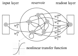
Figure 1: Schematic of a generic reservoir computer. The input is weighted and then fed into a reservoir made up of a number of nodes with nonlinear transfer functions. The nodes are interconnected using the coupling matrix ${\bf W}^{res}=[w^{res}_{ij}]$, where $w^{res}_{ij}$ is the weight from node $j$ to node $i$. The weights are selected randomly from identical and independent distributions. The output is generated using linear combination of the values of the nodes in the reservoir using output weight vector ${\bf W}^{out}=[w^{out}_{i}]$.

Figure 1 shows a sample RC architecture with sparse connectivity between the input and the reservoir, and between the nodes inside the reservoir. The output node is connected to all the reservoir nodes. The input weight matrix is an $I\times N$ matrix ${\bf W}^{in}=[w^{in}_{i,j}]$, where $I$ is the number of input nodes, $N$ is the number of nodes in the reservoir, and $w^{in}_{j,i}$ is the weight of the connection from input node $i$ to reservoir node $j$. The connection weights inside the reservoir are represented by an $N\times N$ matrix ${\bf W}^{res}=[w^{res}_{j,k}]$, where $w^{res}_{j,k}$ is the weight from node $k$ to node $j$ in the reservoir. The output weight matrix is an $N\times O$ matrix ${\bf W}^{out}=[w^{out}_{l,k}]$, where $O$ is the number of output nodes and $w^{out}_{l,k}$ is the weight of the connection from reservoir node $k$ to output node $l$. All the weights are samples of i.i.d. random variables, usually taken to be normally distributed with mean $\mu=0$ and standard deviation $\sigma$. We can tune $\mu$ and $\sigma$ depending on the properties of $U(t)$ to achieve optimal performance. We represent the time-varying input signal by an $I$th order column vector ${\bf U}(t)=[u_{i}(t)]$, the reservoir state by an $N$th order column vector ${\bf X}(t)=[x_{j}(t)]$, and the generated output by an $O$th order column vector ${\bf Y}(t)=[y_{l}(t)]$. We compute the time evolution of each reservoir node in discrete time as:

$$x_{j}(t+1)=f({\bf W}^{res}_{j}\cdot{\bf X}(t)+{\bf W}^{in}\cdot{\bf U}(t)),$$ (1)

where $f$ is the nonlinear transfer function of the reservoir nodes, $\cdot$ is the matrix dot product, and ${\bf W}^{res}_{j}$ is the $j$th row of the reservoir weight matrix. The reservoir output is then given by:

$${\bf Y}(t)=w_{b}+{\bf W}^{out}\cdot{\bf X}(t),$$ (2)

where $w_{b}$ is an inductive bias. One can use any regression method to train the output weights to minimize the output error $E=||{\bf Y}(t)-{\bf\widehat{Y}}(t)||^{2}$ given the target output ${\bf\widehat{Y}}(t)$. We use linear regression and calculate the weights using the Moore-Penrose pseudo-inverse method [10]:

$${\bf W}^{out^{\prime}}=({\bf X^{\prime}}^{T}\cdot{\bf X}^{\prime})^{-1}\cdot{\bf X}^{\prime T}\cdot{\bf Y^{\prime}}.$$ (3)

Here, ${\bf W}^{out^{\prime}}$ is the output weight vector extended with a the bias $w_{b}$, X’ is the matrix of observation from the reservoir state where each row is represent the state of the reservoir at the corresponding time $t$ and the columns represent the state of different nodes extended so that the last column is constant 1. Finally, ${\bf\widehat{Y}^{\prime}}$ is the matrix of target output were each row represents the target output at the corresponding time $t$. Note that this also works for multi-dimensional output, in which case ${\bf W}^{out^{\prime}}$ will be a matrix containing connection weights between each pair of reservoir nodes and output nodes.

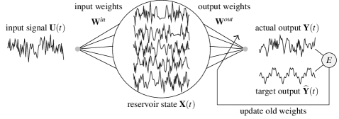
Figure 2: Computation in a reservoir computer. The input signal ${\bf U}(t)$ is fed into every reservoir node $i$ with a corresponding weight $w^{in}_{i}$ denoted with weight column vector ${\bf W}^{in}=[w^{in}_{i}]$. Reservoir nodes are themselves coupled with each other using the weight matrix ${\bf W}^{res}=[w^{res}_{ij}]$, where $w^{res}_{ij}$ is the weight of the connection from node $j$ to node $i$.

Conceptually, the reservoir’s role in RC is to act as a spatiotemporal kernel and project the input into a high-dimensional feature space [6]. In machine learning, this is usually referred to as feature extraction and is done to find hidden structures in data sets or time series. The output is then calculated by properly weighting and combining different features of the data [11]. An ideal reservoir should be able to perform feature extraction in a way that makes the mapping from feature space to output a linear problem. However, this is not always possible. In theory an ideal reservoir computer should have two features: a separation property of the reservoir and an approximation property of the readout layer. The former means the reservoir perturbations from two distinct inputs must remain distinguishable over time and the latter refers to the ability of the readout layer to map the reservoir state to a given target output in a sufficiently precise way.

Another way to understand computation in a high-dimensional recurrent systems is through analyzing their attractors. In this view, the state-space of the reservoir is partitioned into multiple basins of attraction. A basin of attraction is a subspace of the system’s state-space, in which the system follows a trajectory towards its attractor. Thus computation takes place when the reservoir jumps between basins of attraction due to perturbations by an external input [12, 13, 14, 15]. On the other hand, one could directly analyze computation in the reservoir as the reservoir’s average instantaneous information content to produce a desired output [16].

There has been much research to find the optimal reservoir structure and readout strategy. Jaeger [17] suggests that in addition to the separation property, the reservoir should have fading memory to forget past inputs after some period of time. He achieves this by adjusting the standard deviation of the reservoir weight matrix $\sigma$ so that the spectral radius of ${\bf W}^{res}$ remains close to 1, but slightly less than 1. This ensures that the reservoir can operate near critical dynamics, right at the edge between ordered and chaotic regimes. A key feature of critical systems is that perturbations to the system’s trajectory neither spread nor die out, independent of the system size[18], which makes adaptive information processing robust to noise[14]. Other studies have also suggested that the critical dynamics is essential for good performance in RC [19, 20, 16, 21, 22].

The RC architecture does not assume any specifics about the underlying reservoir. The only requirement is that it provides a suitable kernel to project inputs into a high-dimensional feature space. Reservoirs operating in the critical dynamical regime usually satisfy this requirement. Since RC makes no assumptions about the structure of the underlying reservoir, it is very suitable for use with unconventional computing paradigms [3, 4, 5]. Here, we propose and simulate a simple design for a reservoir computer based on a network of deoxyribozyme oscillators.

3 Reservoir Computing using Deoxyribozyme Oscillators

To make a DNA reservoir computer, we first need a reservoir of DNA species with rich transient dynamics. To this end, we use a microfluidic reaction chamber in which different DNA species can interact. This must be an open reactor because we need to continually give input to the system and read its outputs. The reservoir state consists of the time-varying concentration of various species inside the chamber, and we compute using the reaction dynamics of the species inside the reactor. To perturb the reservoir we encode the time-varying input as fluctuations in the influx of species to the reactor. In [23, 2], a network of three deoxyribozyme NOT gates showed stable oscillatory dynamics in an open microfluidic reactor. We extend this work by designing a reservoir computer using deoxyribozyme-based oscillators and investigating their information-processing capabilities.

The oscillator dynamics in [2] suffices as an excitable reservoir. Ideally, the readout layer should also be implemented in a similar microfluidic setting and integrated with the reservoir. However, as a proof of concept we assume that we can read the reservoir state using fluorescent probes and calculate the output weights using software.

The oscillator network in [2] is described using a system of nine ordinary differential equations (ODEs), which simulate the details of a laboratory experiment of the proposed design. However, this model is mathematically unwieldy. We first reduce the oscillator ODEs in [2] to a form more amenable to mathematical analysis:

$$\begin{array}[]{llllllll}\vspace{2mm}\frac{d[P_{1}]}{dt}&=&h\beta[S_{1}]([G_{1}]-[P_{3}])-\frac{e}{V}[P_{1}],&\text{ }&\frac{d[S_{1}]}{dt}&=&\frac{S^{m}_{1}}{V}-h\beta[S_{1}]([G_{1}]-[P_{3}])-\frac{e}{V}[S_{1}],\\ \vspace{2mm}\frac{d[P_{2}]}{dt}&=&h\beta[S_{2}]([G_{2}]-[P_{1}])-\frac{e}{V}[P_{2}],&&\frac{d[S_{2}]}{dt}&=&\frac{S^{m}_{2}}{V}-h\beta[S_{2}]([G_{2}]-[P_{1}])-\frac{e}{V}[S_{2}],\\ \vspace{2mm}\frac{d[P_{3}]}{dt}&=&h\beta[S_{3}]([G_{3}]-[P_{2}])-\frac{e}{V}[P_{3}],&&\frac{d[S_{3}]}{dt}&=&\frac{S^{m}_{3}}{V}-h\beta[S_{3}]([G_{3}]-[P_{2}])-\frac{e}{V}[S_{3}].\end{array}$$ (4)

In this model, $[P_{i}]$, $[S_{i}]$, and $[G_{i}]$ are concentrations of three species of product molecules, three species of substrate molecules, and three species of gate molecules inside the reactor, and $S^{m}_{i}$ is the influx rate of $[S_{i}]$. The brackets $[$ $\cdot$ $]$ indicate chemical concentration and should not be confused with the matrix notation introduced above. When explicitly talking about the concentrations at time $t$, we use $P_{i}(t)$ and $S_{i}(t)$. $V$ is the volume of the reactor, $h$ the fraction of the reactor chamber that is well-mixed, $e$ is the efflux rate, and $\beta$ is the reaction rate constant for the gate-substrate reaction, which is assumed to be identical for all gates and substrates, for simplicity.

To use this system as a reservoir we must ensure that it has transient or sustained oscillation. This can be easily analyzed by forming the Jacobian of the system. Observing that all substrate concentrations reach an identical and constant value relative to their magnitude, we can focus on the dynamics of the product concentrations and write an approximation to the Jacobian of the system as follows:

$${\bf J}=\begin{bmatrix}\vspace{2mm}\frac{d[P_{1}]}{d[P_{1}]}&\frac{d[P_{1}]}{d[P_{2}]}&\frac{d[P_{1}]}{d[P_{3}]}\\ \vspace{2mm}\frac{d[P_{2}]}{d[P_{1}]}&\frac{d[P_{2}]}{d[P_{2}]}&\frac{d[P_{2}]}{d[P_{3}]}\\ \frac{d[P_{3}]}{d[P_{1}]}&\frac{d[P_{3}]}{d[P_{2}]}&\frac{d[P_{3}]}{d[P_{3}]}\end{bmatrix}=\begin{bmatrix}\vspace{2mm}-\frac{e}{V}&-h\beta[S_{1}]&0\\ \vspace{2mm}0&-\frac{e}{V}&-h\beta[S_{2}]\\ -h\beta[S_{1}]&0&-\frac{e}{V}\end{bmatrix}$$ (5)

Assuming that volume of the reactor $V$ and the reaction rate constant $\beta$ are given, the Jacobian is a function of only the efflux rate $e$ and the substrate concentrations $[S_{i}]$. The eigenvalues of the Jacobian are given by:

$$\begin{array}[]{lll}\lambda_{1}&=&-h\beta([S_{1}][S_{2}][S_{3}])^{\frac{1}{3}}-\frac{e}{V}\\ \lambda_{2}&=&\frac{1}{2}h\beta([S_{1}][S_{2}][S_{3}])^{\frac{1}{3}}-\frac{e}{V}+\frac{\sqrt{3}}{2}h\beta([S_{1}][S_{2}][S_{3}])^{\frac{1}{3}}i\\ \lambda_{3}&=&\frac{1}{2}h\beta([S_{1}][S_{2}][S_{3}])^{\frac{1}{3}}-\frac{e}{V}-\frac{\sqrt{3}}{2}h\beta([S_{1}][S_{2}][S_{3}])^{\frac{1}{3}}i\end{array}$$ (6)

The existence of complex eigenvalues tells us that the system has oscillatory behavior near its critical points. The period of this oscillation is given by $T=2\pi\frac{\sqrt{3}}{2}h\beta([S_{1}][S_{2}][S_{3}])^{-\frac{1}{3}}$ and can be adjusted by setting appropriate base values for $S^{m}_{i}$. For sustained oscillation, the real part of the eigenvalues should be zero, which can be obtained by a combination of efflux rate and substrate influx rates such that $\frac{1}{2}h\beta([S_{1}][S_{2}][S_{3}])^{\frac{1}{3}}-\frac{e}{V}=0$.

This model works as follows. The substrate molecules enter the reaction chamber and are bound to and cleaved by active gate molecules that are immobilized inside the reaction chamber, e.g., on beads. This reaction turns substrate molecules into the corresponding product molecule. However, the presence of each product molecule concentration suppresses the reaction of other substrates and gates. These three coupled reaction and inhibition cycles give rise to the oscillatory behavior of the products’ concentrations (Figure 4). Input is given to the system as fluctuation to one or more of the substrate influx rates. In Figure 3a we see that the concentration of $S_{1}$ varies rapidly as a response to the random fluctuations in $S^{m}_{1}$. This will result in antisymmetric concentrations of the substrate species inside the chamber and thus irregular oscillation of the concentration of product molecules. This irregular oscillation embeds features of the input fluctuation within it (Figure 3a). To keep the volume fixed, there is a continuous efflux of the chamber content. The Equation 4 assumes $([G_{i}]-[P_{j}])>0$, which should be taken into account while choosing initial concentrations and constants to simulate the system.

To perturb the intrinsic dynamics inside the reactor, an input signal can modulate one or more substrate influx rates. In our system, we achieve this by fluctuating $S^{m}_{1}$. In order to let the oscillators react to different values of $S^{m}_{i}$, we keep each new value of $S^{m}_{i}$ constant for $\tau$ seconds. In a basic setup, the initial concentrations of all the substrates inside the reactor are zero. Two of the product concentrations $P_{2}(0)$ and $P_{3}(0)$ are also set to zero, but to break the symmetry in the system and let the oscillation begin we set $P_{1}(0)=1000$ nM. The gate concentrations are set uniformly to $[G_{i}]=2500$ nM. This ensures that $([G_{i}]-[P_{j}])>0$ in our setup. The base values for substrate-influx rates are set to $5.45\times 10^{-6}$ nmol s^-1. Figure 3 shows the traces of computer simulation of this model, where $\tau=30$ s. We use the reaction rate constant from [2], $\beta=5\times 10^{-7}$ nM s^-1. Although the kinetics of immobilized deoxyribozyme may be different, for simplicity we use the reaction rate constant of free deoxyribozymes and we assume that we can find deoxyribozymes with appropriate kinetics when immobilized. The values for the remaining constants are $e=8.8750\times 10^{-2}$ nL s^-1 and $h=0.7849$, i.e., the average fraction of well-mixed solution calculated in [2]. We assume the same microscale continuous stirred-tank reactor ($\mu$CSTR) as [2, 23, 24], which has volume $V=7.54$ nL. The small volume of the reactor lets us achieve high concentration of oligonucleotides with small amounts of material; a suitable experimental setup is described in [25].

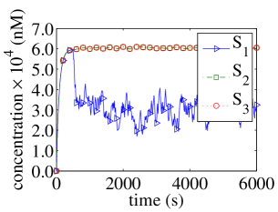
(a) substrate in the reduced model

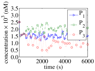
(b) products in the reduced model

Figure 3: The random fluctuation in substrate influx rate $S^{m}_{1}$ leaves traces on the oscillator dynamics that can be read off a readout layer. We observe the traces of the substate influx rate fluctuation both in the dynamics of the substrate concentrations LABEL:sub@fig:subflucredo and the product concentrations LABEL:sub@fig:prodflucredo. Both substrate and product concentrations potentially carry information about the input. Substrate concentration $S_{1}$ is directly affected by $S^{m}_{1}$ and therefore shows very rapid fluctuations.

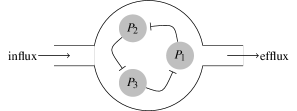
Figure 4: Three products form an inhibitory cycle that leads to oscillatory behavior in the reservoir. Each product $P_{i}$ inhibits the production of $P_{i+1}$ by the corresponding deoxyribozyme (cf. Equation 4).

The dynamics of the substrates (Figure 3a) and products (Figure 3a) are instructive as to what we can use as our reservoir state. Our focus will be the product concentrations. However, the substrate concentrations also show interesting irregular behavior that can potentially carry information about the input signals. This is not surprising since all of the substrate and product concentrations are connected in our oscillator network. However, the one substrate that is directly affected by the influx ($S_{1}$ in this case) shows the most intense fluctuations that are directly correlated with the input. In some cases providing this extra information to the readout layer can help to find the right mapping between the reservoir state and the target output.

In the next section, we build two different reservoir computers using the dynamics of the concentrations in the reactor and use them to solve sample temporal tasks. Despite the simplicity of our system, it can retain the memory of past inputs inside the reservoir and use it to produce output.

4 Task Solving Using a Deoxyribozyme Reservoir Computer

We saw in the preceding section that we can use substrate influx fluctuation as input to our molecular reservoir. We now show that we can train a readout layer to map the dynamics of the oscillator network to a target output. Recall that $\tau$ is the input hold time during which we keep $S^{m}_{1}$ constant so that the oscillators can react to different values of $S^{m}_{1}$. In other words, at the beginning of each $\tau$ interval a new random value for substrate influx is chosen and held fixed for $\tau$ seconds. Here, we set the input hold time $\tau=100$ s. In addition, before computing with the reservoir we must make sure that it has settled in its natural dynamics, otherwise the output layer will see dynamical behavior that is due to the initial conditions of the oscillators and not the input provided to the system. In the model, the oscillators reach their stable oscillation pattern within $500$ s. Therefore, we start our reservoir by using a fixed $S^{m}_{1}$ as described in Section 3 and run it for $500$ s before introducing fluctuations in $S^{m}_{1}$.

To study the performance of our DNA reservoir computer we use two different tasks, Task A and Task B, as toy problems. Both have recursive time dependence and therefore require the reservoir to remember past inputs for some period of time, and both are simplified versions of a popular RC benchmark, NARMA [8]. We define the input as $S^{m}_{1}(t)=S^{m*}_{1}R$, where $S^{m*}_{1}$ is the influx rate used for the normal working of the oscillators ($5.45\times 10^{-6}$ nmol s^-1 in our experiment) and $R$ is a random value between 0 and 1 sampled from a uniform distribution. We define the target output ${\bf\widehat{Y}(t)}$ of Task A as follows:

$${\bf\widehat{Y}}(t)=S^{m}_{1}(t-1)+2S^{m}_{1}(t-2).$$ (7)

For Task B, we increase the length of the time dependence and make it a function of input hold time $\tau$. We define the target output as follows:

$${\bf\widehat{Y}}(t)=S^{m}_{1}(t-\tau)+\frac{1}{2}S^{m}_{1}(t-\frac{3}{2}\tau).$$ (8)

Note that the vectors ${\bf\widehat{Y}}(t)$ and ${\bf Y}(t)$ have only one row in this example. Figure 5 shows an example of the reservoir output ${\bf Y}(t)$ and the target output ${\bf\widehat{Y}}(t)$ calculated using Equation 7 before and after training. In this example, the reservoir output before training is $10$ orders of magnitude off the target.

Our goal is to find a set of output weights so that ${\bf Y}(t)$ tracks the target output as closely as possible. We calculate the error using normalized root-mean-square error (NRMSE) as follows:

$$\text{NRMSE}=\frac{1}{Y_{max}-Y_{min}}\sqrt{\frac{\sum_{t=t_{1}}^{t_{n}}({\bf\widehat{Y}}(t)-{\bf Y}(t))^{2}}{n}},$$ (9)

where $Y_{max}$ and $Y_{min}$ are the maximum and the minimum of the ${\bf Y}(t)$ during the time interval $t_{1}<t<t_{n}$. The denominator $Y_{max}-Y_{min}$ is to ensure that $0\leq\text{NRMSE}\leq 1$, where $\text{NRMSE}=0$ means ${\bf Y}(t)$ matches ${\bf\widehat{Y}}(t)$ perfectly.

Now we propose two different ways of calculating the output from the reservoir: (1) using only the dynamics of the product concentrations and (2) using both the product and substrate concentrations. To formalize this using the block matrix notation, for the product-only version the reservoir state is given by ${\bf X}(t)={\bf P}(t)=[P_{1}(t)\text{ }P_{2}(t)\text{ }P_{3}(t)]^{T}$. For the product-and-substrate version the reservoir state is given by vertically appending ${\bf S}(t)=[S_{1}(t)\text{ }S_{2}(t)\text{ }S_{3}(t)]^{T}$ to ${\bf P}(t)$, i.e., ${\bf X}(t)=[{\bf P}(t)\text{ }{\bf S}(t)]^{T}$, where ${\bf P}(t)$ is the column vector of the product concentrations as before and ${\bf S}(t)$ is the column vector of the substrate concentrations. We use $2000$ s of the reservoir dynamics ${\bf X}(t)$ to calculate the output weight matrix ${\bf W}^{out}$ using linear regression. We then test the generalization, i.e., how well the output ${\bf Y}(t)$ tracks the target ${\bf\widehat{Y}}(t)$ during another $2000$ s period that we did not use to calculate the weights.

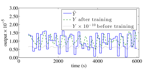
Figure 5: Target output and the output of the molecular reservoir computer on Task A (Equation 7) before and after training. After $500$ s the input starts to fluctuate randomly every $\tau$ seconds. In this example, the output of the system before training is 10 orders of magnitude larger than the target output. We rescaled the output before training to be able to show it in this plot. After training, the output is in the range of the target output and it tracks the fluctuations in the target output more closely.

Figure 6 shows the mean and standard deviation of NRMSE of the reservoir computer using two different readout layer solving Task A and Task B. The product-and-substrate reservoir achieves a mean NRMSE of $0.23$ and $0.11$ on Task A and Task B with standard deviations $0.05$ and $0.02$ respectively, and the product-only reservoir achieves a mean NRMSE of $0.30$ and $0.19$ on Task A and Task B with standard deviations $0.04$ and $0.03$ respectively. As expected, the product-and-substrate reservoir computer achieves about $10\%$ improvement over the product-only version owing to its higher phase space dimensionality. Furthermore, both reservoirs achieve a $10\%$ improvement on Task B over Task A. This is surprising at first because Task B requires the reservoir to remember the input over a time interval of $\frac{3}{2}\tau$, but Task A only requires the last two time steps. However, to extract the features in the input signal, the input needs to percolate in the reservoir, which takes more than just two time steps. Task B requires more memory of the input, but also gives the reservoir enough time to process the input signal, which results in higher performance. Similar effects have been observed in [16]. Therefore, despite the very simple reservoir structure (three coupled oscillators), we can compute simple temporal tasks with $90\%$ accuracy. Increasing the number of oscillators and using the history of the oscillators dynamics similar to [26] could potentially lead to even higher performance.

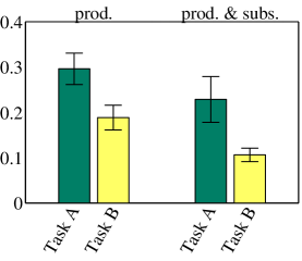
Figure 6: Generalization NRMSE of the product-only and the product-and-substrate molecular reservoir computer on Task A (Equation 7) and Task B (Equation 8) averaged over $100$ trials. The bars and error bars show the mean and the standard deviation of NRMSE respectively.

5 Discussion and Related Work

DNA chemistry is inherently programmable and highly versatile, and a number of different techniques have been developed, such as building digital and analog circuits using strand displacement cascades [27, 28], developing game-playing molecular automata using deoxyribozymes [29], and directing self-assembly of nanostructures   [30, 31, 32]. All of these approaches require precise design of DNA sequences to form the required structures and perform the desired computation. In this paper, we proposed a reservoir-computing approach to molecular computing. In nature, evidence for reservoir computing has been found in systems as simple as a bucket of water [33], simple organisms such as E. Coli [34], and in systems as complex as the brain [35]. This approach does not require any specific behavior from the reactions, except that the reaction dynamics must result in a suitable transient behavior that we can use to compute [6]. This could give us a new perspective in long-term sensing, and potentially controlling, gene expression patterns over time in a cell. This would require appropriate sensors to detect cell state, for example the pH-sensitive DNA nanomachine recently reported by Modi et al. [36]. This may result in new methods for smart diagnosis and treatment using DNA signal translators [37, 38, 39].

In RC, computation takes place as a transformation from the input space to a high- dimensional spatiotemporal feature space created by the transient dynamics of the reservoir. Mathematical analysis suggests that all dynamical systems show the same information processing capacity [40]. However, in practice, the performance of a reservoir is significantly affected by its dynamical regime. Many studies have shown that to achieve a suitable reservoir in general, the underlying dynamical system must operate in the critical dynamical regime [16, 8, 20, 21].

We used the dynamics of the concentrations of different molecular species to extract features of an input signal and map them to a desired output. As a proof of concept, we proposed a reservoir computer using deoxyribozyme oscillator network and showed how to provide it with input and read its outputs. However, in our setup, we assumed that we read the reservoir state using fluorescent probes and process them using software. In principle, the mapping from the reservoir state to target output can be carried out as an integrated part of the chemistry using an approach similar to the one reported in [28], which implements a neural network using strand displacement. In[41], we proposed a chemical reaction network inspired by deoxyribozyme chemistry that can learn a linear function and repeatedly use it to classify input signals. In principle, these methods could be used to implement the regression algorithm and therefore the readout layer as an integrated part of the molecular reservoir computer. A microfluidic reactor has been demonstrated in [25] that would be suitable for implementing our system. Therefore, the molecular reservoir computer that we proposed here is physically plausible and can be implemented in the laboratory using microfuidics.

6 Conclusion and Future Work

We have proposed and simulated a novel approach to DNA computing based on the reservoir computing paradigm. Using a network of oscillators built from deoxyribozymes we can extract hidden features in a given input signal and compute any desired output. We tested the performance of this approach on two simple temporal tasks. This approach is generalizable to different molecular species so long as they possess rich reaction dynamics. Given the available technology today this approach is plausible and can lead to many innovations in biological signal processing, which has important applications in smart diagnosis and treatment techniques. In future work, we shall study the use of other sets of reactions for the reservoir. Moreover, for any real-world application of this technique, we have to address the chemical implementation of the readout layer. An important open question is the complexity of molecular reactions necessary to achieve critical dynamics in the reservoir. For practical applications, the effect of sparse input and sparse readout needs thorough investigation, i.e., how should one distribute the input to the reservoir and how much of the reservoir dynamics is needed for the readout layer to reconstruct the target output accurately? It is also possible to use the history of the reservoir dynamics to compute the output, which would require addition of a feedback channel to the reactor. The molecular readout layer could be set up to read the species concentration along the feedback channel. Another possibility is to connect many reactors to create a modular molecular reservoir computer, which could be used strategically to scale up to more complex problems.

References

- [1] Jaeger, H., Haas, H.: Harnessing nonlinearity: Predicting chaotic systems and saving energy in wireless communication. Science 304(5667) (2004) 78–80
- [2] Farfel, J., Stefanovic, D.: Towards practical biomolecular computers using microfluidic deoxyribozyme logic gate networks. In Carbone, A., Pierce, N., eds.: DNA Computing. Volume 3892 of Lecture Notes in Computer Science. Springer Berlin Heidelberg (2006) 38–54
- [3] Lukoševičius, M., Jaeger, H., Schrauwen, B.: Reservoir computing trends. KI - Künstliche Intelligenz 26(4) (2012) 365–371
- [4] Smerieri, A., Duport, F., Paquot, Y., Schrauwen, B., Haelterman, M., Massar, S.: Analog readout for optical reservoir computers. In Bartlett, P., Pereira, F., Burges, C., Bottou, L., Weinberger, K., eds.: Advances in Neural Information Processing Systems 25: 26th Annual Conference on Neural Information Processing Systems. Curran Associates, Inc. (2012) 953–961
- [5] Paquot, Y., Duport, F., Smerieri, A., Dambre, J., Schrauwen, B., Haelterman, M., Massar, S.: Optoelectronic reservoir computing. Scientific Reports 2 (2012)
- [6] Lukoševičius, M., Jaeger, H.: Reservoir computing approaches to recurrent neural network training. Computer Science Review 3(3) (2009) 127–149
- [7] Maass, W., Natschläger, T., Markram, H.: Real-time computing without stable states: a new framework for neural computation based on perturbations. Neural computation 14(11) (2002) 2531–60
- [8] Jaeger, H.: Tutorial on training recurrent neural networks, covering BPPT, RTRL, EKF and the ‚“echo state network‚” approach. Technical Report GMD Report 159, German National Research Center for Information Technology, St. Augustin-Germany (2002)
- [9] Widrow, B., Lehr, M.: 30 years of adaptive neural networks: Perceptron, madaline, and backpropagation. Proceedings of the IEEE 78(9) (1990) 1415–1442
- [10] Penrose, R.: A generalized inverse for matrices. Mathematical Proceedings of the Cambridge Philosophical Society 51 (1955) 406–413
- [11] Bishop, C.M.: Pattern Recognition and Machine Learning (Information Science and Statistics). Springer-Verlag New York, Inc., Secaucus, NJ, USA (2006)
- [12] Sussillo, D., Barak, O.: Opening the black box: Low-dimensional dynamics in high-dimensional recurrent neural networks. Neural Computation 25(3) (2012) 626–649
- [13] Sussillo, D., Abbott, L.F.: Generating coherent patterns of activity from chaotic neural networks. Neuron 63(4) (2009) 544–557
- [14] Goudarzi, A., Teuscher, C., Gulbahce, N., Rohlf, T.: Emergent criticality through adaptive information processing in Boolean networks. Phys. Rev. Lett. 108 (2012) 128702
- [15] Krawitz, P., Shmulevich, I.: Basin entropy in boolean network ensembles. Phys. Rev. Lett. 98(15) (2007) 158701
- [16] Snyder, D., Goudarzi, A., Teuscher, C.: Computational capabilities of random automata networks for reservoir computing. Phys. Rev. E 87 (2013) 042808
- [17] Jaeger, H.: Short term memory in echo state networks. Technical Report GMD Report 152, GMD-Forschungszentrum Informationstechnik (2002)
- [18] Rohlf, T., Gulbahce, N., Teuscher, C.: Damage spreading and criticality in finite random dynamical networks. Phys. Rev. Lett. 99(24) (2007) 248701
- [19] Natschläger, T., Maass, W.: Information dynamics and emergent computation in recurrent circuits of spiking neurons. In Thrun, S., Saul, L., Schoelkpf, B., eds.: Proc. of NIPS 2003, Advances in Neural Information Processing Systems. Volume 16., Cambridge, MIT Press (2004) 1255–1262
- [20] Bertschinger, N., Natschläger, T.: Real-time computation at the edge of chaos in recurrent neural networks. Neural Computation 16(7) (2004) 1413–1436
- [21] Büsing, L., Schrauwen, B., Legenstein, R.: Connectivity, dynamics, and memory in reservoir computing with binary and analog neurons. Neural Computation 22(5) (2010) 1272–1311
- [22] Boedecker, J., Obst, O., Mayer, N.M., Asada, M.: Initialization and self-organized optimization of recurrent neural network connectivity. HFSP Journal 3(5) (2009) 340–349
- [23] Morgan, C., Stefanovic, D., Moore, C., Stojanovic, M.N.: Building the components for a biomolecular computer. In Ferretti, C., Mauri, G., Zandron, C., eds.: DNA Computing. Volume 3384 of Lecture Notes in Computer Science. Springer Berlin Heidelberg (2005) 247–257
- [24] Chou, H.P., Unger, M., Quake, S.: A microfabricated rotary pump. Biomedical Microdevices 3(4) (2001) 323–330
- [25] Galas, J.C., Haghiri-Gosnet, A.M., Estevez-Torres, A.: A nanoliter-scale open chemical reactor. Lab Chip 13 (2013) 415–423
- [26] Appeltant, L., Soriano, M.C., Van der Sande, G., Danckaert, J., Massar, S., Dambre, J., Schrauwen, B., Mirasso, C.R., Fischer, I.: Information processing using a single dynamical node as complex system. Nature Communications 2 (2011)
- [27] Qian, L., Winfree, E.: Scaling up digital circuit computation with DNA strand displacement cascades. Science 332(6034) (2011) 1196–1201
- [28] Qian, L., Winfree, E., Bruck, J.: Neural network computation with DNA strand displacement cascades. Nature 475(7356) (2011) 368–372
- [29] Pei, R., Matamoros, E., Liu, M., Stefanovic, D., Stojanovic, M.N.: Training a molecular automaton to play a game. Nature Nanotechnology 5(11) (2010) 773–777
- [30] Yin, P., Choi, H.M.T., Calvert, C.R., Pierce, N.A.: Programming biomolecular self-assembly pathways. Nature 451(7176) (2008) 318–322
- [31] Wei, B., Dai, M., Yin, P.: Complex shapes self-assembled from single-stranded DNA tiles. Nature 485(7400) (2012) 623–626
- [32] Ke, Y., Ong, L.L., Shih, W.M., Yin, P.: Three-dimensional structures self-assembled from DNA bricks. Science 338(6111) (2012) 1177–1183
- [33] Fernando, C., Sojakka, S.: Pattern recognition in a bucket. In Banzhaf, W., Ziegler, J., Christaller, T., Dittrich, P., Kim, J., eds.: Advances in Artificial Life. Volume 2801 of Lecture Notes in Computer Science. Springer Berlin Heidelberg (2003) 588–597
- [34] Jones, B., Stekel, D., Rowe, J., Fernando, C.: Is there a liquid state machine in the bacterium Escherichia coli? In: Artificial Life, 2007. ALIFE ’07. IEEE Symposium on. (2007) 187–191
- [35] Yamazaki, T., Tanaka, S.: The cerebellum as a liquid state machine. Neural Networks 20(3) (2007) 290–297
- [36] Modi, S., Nizak, C., Surana, S., Halder, S., Krishnan, Y.: Two DNA nanomachines map pH changes along intersecting endocytic pathways inside the same cell. Nat Nano 8(6) (2013) 459–467
- [37] Beyer, S., Dittmer, W., Simmel, F.: Design variations for an aptamer-based DNA nanodevice. Journal of Biomedical Nanotechnology 1(1) (2005) 96–101
- [38] Beyer, S., Simmel, F.C.: A modular DNA signal translator for the controlled release of a protein by an aptamer. Nucleic Acids Research 34(5) (2006) 1581–1587
- [39] Shapiro, E., Gil, B.: RNA computing in a living cell. Science 322(5900) (2008) 387–388
- [40] Dambre, J., Verstraeten, D., Schrauwen, B., Massar, S.: Information processing capacity of dynamical systems. Scientific Reports 2 (2012)
- [41] Lakin, M.R., Minnich, A., Lane, T., Stefanovic, D.: Towards a biomolecular learning machine. In Durand-Lose, J., Jonoska, N., eds.: Unconventional Computation and Natural Computation 2012. Volume 7445 of Lecture Notes in Computer Science., Springer-Verlag (2012) 152–163