Multi-Parameter Tikhonov Regularization
– An Augmented Approach

Abstract

We study multi-parameter regularization (multiple penalties) for solving linear inverse problems to promote simultaneously distinct features of the sought-for objects. We revisit a balancing principle for choosing regularization parameters from the viewpoint of augmented Tikhonov regularization, and derive a new parameter choice strategy called the balanced discrepancy principle. A priori and a posteriori error estimates are provided to theoretically justify the principles, and numerical algorithms for efficiently implementing the principles are also provided. Numerical results on denoising are presented to illustrate the feasibility of the balanced discrepancy principle.
Keywords: multi-parameter regularization, augmented Tikhonov regularization, balanced discrepancy principle

1 Introduction

We investigate a regularization technique for robustly solving linear inverse problems modeled by

(1) $$Ku^{\dagger}=g^{\dagger},$$

where $g^{\dagger}$ is the (inaccessible) exact data and $u^{\dagger}\in X$ represents the unknown exact solution, and $K:X\rightarrow Y$ is a bounded linear operator. Here the spaces $X$ and $Y$ are general Banach spaces, and the operator $K$ can be an embedding operator (image denoising), a convolution operator (deblurring, scattering) and the Radon transform (computed tomography). The objective is to find an approximation $u$ to the solution $u^{\dagger}$ from noisy measurement $g^{\delta}\in Y$ of the exact data $g^{\dagger}$. The accuracy of the noisy data $g^{\delta}$ is measured by the standard $\mathrm{L}^{2}$ fidelity functional $\phi(u^{\dagger},g^{\delta})=\frac{1}{2}\|Ku^{\dagger}-g^{\delta}\|^{2}=\frac{1}{2}\delta^{2}$ with the noise level $\delta$.

As is typical for many inverse problems, problem (1) suffers from ill-posedness or instability. This poses significant challenges to their accurate yet stable numerical solution in the presence of data noise, which is often the case in practical applications. Often, regularization is applied to find a stable approximate solution. One of the most widely used approaches is known as Tikhonov regularization. It seeks to minimize the following functional

(2) $$J_{\boldsymbol{\eta}}(u)=\phi(u,g^{\delta})+\boldsymbol{\eta}\cdot\boldsymbol{\psi}(u),$$

over a closed convex feasible solution set $\mathcal{C}$. The solution to the minimization problem, denoted by $u_{\mathcal{\boldsymbol{\eta}}}^{\delta}$ ($u_{\boldsymbol{\eta}}$ in case of the exact data $g^{\dagger}$), serves as an approximation to the exact solution $u^{\dagger}$. Here the (nonnegative) vector-valued penalty functional $\boldsymbol{\psi}$ encodes the a priori knowledge, and $\boldsymbol{\eta}\cdot\boldsymbol{\psi}(u)$ denotes the dot product between the regularization parameter vector $\boldsymbol{\eta}=(\eta_{1},\eta_{2})^{\mathrm{t}}\in\mathbb{R}^{2}_{+}$ and the penalty $\boldsymbol{\psi}(u)=(\psi_{1}(u),\psi_{2}(u))^{\mathrm{t}}$. The penalty $\boldsymbol{\psi}$ is selected to promote desirable features of the sought-for solution, e.g., edge, sparsity and texture; and often the optimization problem (2) is nonsmooth. The (vector) parameter $\boldsymbol{\eta}$ compromises the fidelity $\phi$ with the penalty $\boldsymbol{\psi}$, and its appropriate choice plays a crucial role in obtaining stable yet accurate solutions. Therefore, an automated selection rule and efficient algorithms for determining $\boldsymbol{\eta}$ are essential.

One distinct feature of the model (2) is that it includes multiple penalties (hence termed as multi-parameter regularization). This is motivated by the following empirical observations. In practice, many objects exhibit distinct multiple features/structures. However, one single penalty generally favors one feature over others, and thus unsuitable for promoting multiple distinct features. For example, total variation ($\mathrm{TV}$) is well suited to reconstructing piecewise constant structures, however, it results in significant staircases in gray regions. One may improve $\mathrm{TV}$-reconstruction by introducing an additional penalty, say $\mathrm{L}^{1}$ norm of $\Delta u$ where $\Delta$ is the Laplacian operator. Hence, a reliable recovery of several distinct features naturally calls for multiple penalties, and it is not surprising that the idea of multi-parameter regularization has been pursued earlier. For instance, in [9] the authors proposed a model to preserve both flat and gray regions in natural images by combining $\mathrm{TV}$ with Sobolev smooth penalty. We refer interested readers to [17, 15] (imaging), [19] (microarray data analysis), [18] (geodesy) and [13] (machine learning) for other interesting applications.

However, a general theory of multi-parameter regularization remains under development [1, 4, 13, 7]. In [1] the $L$-hypersurface was suggested for determining regularization parameters for finite-dimensional linear systems, but without any theoretical justification. In [4], a multi-resolution analysis for ill-posed linear operator equations was analyzed, and some convergence results were established. Lu et al. [13] discussed the discrepancy principle for Hilbert space scales, and derived some error estimates. However, the parameter selection is vastly nonunique due to lack of constraints and thus not directly applicable in practice, for which later a quasi-optimality criterion was suggested [14]. Recently, the authors [7] investigated the discrepancy principle and a balancing principle for general convex variational models. However, the nonuniqueness of the discrepancy principle remains unresolved, and further, there is still no theory for the balancing principle for multi-parameter regularization.

The present work extends our earlier work [7], and includes the following essential contributions. We first revisit the balancing principle in [7] from the viewpoint of augmented Tikhonov regularization [12], and established the equivalence. Then we derive a novel hybrid principle, the balanced discrepancy principle, by incorporating constraints into the augmented approach, which partially resolves the nonuniqueness issue. Further, a priori and a posterior error estimate are derived for both principles. The estimate in Theorem 2.4 was stated in [7] without a proof. Finally, we develop efficient algorithms for implementing these principles, and briefly discuss their properties.

The rest of the paper is organized as follows. In §2, we derive the balancing principle and the new hybrid principle, and develop relevant error estimates. In §3 we discuss efficient implementations of the two principles. Finally, we provide some numerical results to illustrate the hybrid principle in §4.

2 An augmented approach

The augmented Tikhonov (a-Tikhonov) regularization is one principled framework for choosing regularization parameters [12]. Here we describe the augmented approach for multi-parameter models, and derive the balancing principle and a novel balanced discrepancy principle.

2.1 Derivation of the principles

2.1.1 Balancing principle

First we sketch the augmented approach. For the multi-parameter model (2), it can be derived analogously from hierarchical Bayesian inference as in [12], and the resulting augmented functional $J(u,\tau,\boldsymbol{\lambda})$ reads

$$J(u,\tau,\boldsymbol{\lambda})=\tau\phi(u,g^{\delta})+\boldsymbol{\lambda}\cdot\boldsymbol{\psi}(u)+\boldsymbol{e}\cdot(\beta\boldsymbol{\lambda}-\alpha\ln\boldsymbol{\lambda})+\beta_{0}\tau-\alpha_{0}\ln\tau,$$

where the vector $\boldsymbol{e}$ is given by $\boldsymbol{e}=(1,1)^{\mathrm{t}}$. The functional $J(u,\tau,\boldsymbol{\lambda})$ maximizes the posteriori probability density function

$$p(u,\tau,\boldsymbol{\lambda}|g^{\delta})\propto\,p(g^{\delta}|u,\tau,\boldsymbol{\lambda})\,p(u,\tau,\boldsymbol{\lambda}).$$

The functional $J(u,\tau,\boldsymbol{\lambda})$ is derived under the assumption that the scalars $\lambda_{i}$ and $\tau$ have Gamma distributions with known parameter pairs. The parameter pairs $(\alpha,\beta)$ and $(\alpha_{0},\beta_{0})$ are related to the shape parameters in the statistical priors on the prior precision $\lambda_{i}$ and noise precision $\tau$, respectively. The special case $\beta_{0}=\beta=0$ is known as noninformative prior and customarily adopted in practice. Hence we focus our derivation on this case. Upon letting $\eta_{i}=\frac{\lambda_{i}}{\tau}$, the necessary optimality condition of any minimizer $(u_{\boldsymbol{\eta}}^{\delta},\lambda_{i},\tau)$ to the a-Tikhonov functional $J(u,\tau,\{\lambda_{i}\})$ is given by

(3) $$\left\{\begin{aligned} u^{\delta}_{\boldsymbol{\eta}}&=\arg\min_{u\in\mathcal{C}}\;\left\{\phi(u,g^{\delta})+\boldsymbol{\eta}\cdot\boldsymbol{\psi}(u)\right\},\\ \lambda_{i}&=\dfrac{\alpha}{\psi_{i}(u^{\delta}_{\boldsymbol{\eta}})},\quad i=1,2,\\ \tau&=\dfrac{\alpha_{0}}{\phi(u_{\boldsymbol{\eta}}^{\delta},g^{\delta})}.\end{aligned}\right.$$

Now by rewriting the system with $\gamma=\frac{\alpha_{0}}{\alpha}$, we arrive at the following system for $(u^{\delta}_{\boldsymbol{\eta}},{\boldsymbol{\eta}})$

(4) $$\left\{\begin{aligned} &u^{\delta}_{\boldsymbol{\eta}}=\arg\min_{u\in\mathcal{C}}\;\left\{\phi(u,g^{\delta})+{\boldsymbol{\eta}}\cdot{\boldsymbol{\psi}}(u)\right\},\\ &\eta_{i}=\frac{1}{\gamma}\frac{\phi(u^{\delta}_{\boldsymbol{\eta}},g^{\delta})}{\psi_{i}(u^{\delta}_{\boldsymbol{\eta}})},\ i=1,2.\end{aligned}\right.$$

The optimality system (4) reveals the mechanism of the augmented approach: it selects an optimal regularization parameter $\boldsymbol{\eta}$ in the model (2) by balancing the penalty $\boldsymbol{\psi}$ with the fidelity $\phi$, from which the term balancing principle follows. We note the term balancing principle here should not be confused with Lepskii’s principle, which is also sometimes called a balancing principle [16]. The Lepskii’s principle does require a knowledge of noise level.

Next we characterize (4) using the value function $F(\boldsymbol{\eta})$ [8] defined by

$$F(\boldsymbol{\eta})=\inf_{u\in\mathcal{C}}J_{\boldsymbol{\eta}}(u).$$

The function $F(\boldsymbol{\eta})$ is continuous, and it is almost everywhere differentiable, cf. Lemma 2.1. We denote by $F_{\eta_{i}}$ the partial derivative of $F(\boldsymbol{\eta})$ with respect to $\eta_{i}$. The proof is analogous to [8], and hence omitted.

Lemma 2.1.

The function $F(\boldsymbol{\eta})$ is monotone and concave, and hence almost everywhere differentiable. Further, if it is differentiable, then there holds $F_{\eta_{i}}(\boldsymbol{\eta})=\psi_{i}(u_{\boldsymbol{\eta}}^{\delta}).$

Next we provide an alternative characterization of (4). First we define the function $\Phi_{\gamma}(\boldsymbol{\eta})$ by

(5) $$\Phi_{\gamma}({\boldsymbol{\eta}})=\frac{F({\boldsymbol{\eta}})^{\gamma+2}}{\eta_{1}\eta_{2}}.$$

The necessary optimality condition for $\Phi_{\gamma}({\boldsymbol{\eta}})$, provided that $F({\boldsymbol{\eta}})$ is differentiable, reads

$$\dfrac{\partial\Phi_{\gamma}}{\partial\eta_{i}}=\dfrac{F({\boldsymbol{\eta}})^{\gamma+1}}{\eta_{1}\eta_{2}}\dfrac{\left(-F({\boldsymbol{\eta}})+(2+\gamma)\eta_{i}F_{\eta_{i}}({\boldsymbol{\eta}})\right)}{\eta_{i}}=0,\quad i=1,2$$

which, upon noting Lemma 2.1, is equivalent to

$$\left\{\begin{array}[]{l}-\phi(u_{\boldsymbol{\eta}}^{\delta},g^{\delta})+(1+\gamma)\eta_{1}\psi_{1}(u_{\boldsymbol{\eta}}^{\delta})-\eta_{2}\psi_{2}(u_{\boldsymbol{\eta}}^{\delta})=0,\\ \\ -\phi(u_{\boldsymbol{\eta}}^{\delta},g^{\delta})-\eta_{1}\psi_{1}(u_{\boldsymbol{\eta}}^{\delta})+(1+\gamma)\eta_{2}\psi_{2}(u_{\boldsymbol{\eta}}^{\delta})=0.\end{array}\right.$$

Solving the system with respect to $\eta_{i}$ yields $\eta_{i}=\frac{1}{\gamma}\frac{\phi(u_{\boldsymbol{\eta}}^{\delta},g^{\delta})}{\psi_{i}(u_{\boldsymbol{\eta}}^{\delta})}$. Hence, the optimality system of the function $\Phi_{\gamma}$ coincides with that of the functional $J(u,\tau,\boldsymbol{\lambda})$. In summary, we have shown our first main result.

Proposition 2.1.

Let the value function $F(\boldsymbol{\eta})$ be differentiable. Then all critical points of the function $\Phi_{\gamma}$ are solutions to system (4).

Remark 2.1.

Two remarks on the function $\Phi_{\gamma}$ are in order. First, it is very flexible in that the free-parameter $\gamma$ may be calibrated to achieve specific desirable properties. Second, by the concavity in Lemma 2.1, $F(\boldsymbol{\eta})$ is continuous and thus the problem of minimizing $\Phi_{\gamma}$ over any bounded and closed region in $\mathbb{R}^{2}_{+}$ is well defined. These observations remain valid for a general fidelity.

2.1.2 Balanced discrepancy principle

To solve stably and accurately problem (1), one should use all prior information, e.g., the noise level $\phi(u^{\dagger},g^{\delta})=c:=\frac{1}{2}c_{m}^{2}\delta^{2}$ for some $c_{m}\geq 1$, and other relevant knowledge, whenever it is available. This can be realized by incorporating constraints into the augmented approach, and then deriving the corresponding optimal system. For instance, for the constraint $\phi(u,g^{\delta})\leq c$, the Lagrangian approach gives the following a-Tikhonov functional

$$J(u,\tau,\boldsymbol{\lambda},\mu)=\tau\phi(u,g^{\delta})+ \boldsymbol{\lambda}\cdot\boldsymbol{\psi}(u)-\alpha\boldsymbol{e}\cdot\ln\boldsymbol{\lambda}-\alpha_{0}\ln\tau+\tau\langle\phi(u,g^{\delta})-c,\mu\rangle,$$

where the unknown scalar $\mu\geq 0$ is the Lagrange multiplier for the inequality constraint $\phi(u,g^{\delta})\leq c$. Its optimality system reads

$$\left\{\begin{aligned} u^{\delta}_{\boldsymbol{\eta}}&=\arg\min_{u}\;\left\{\phi(u,g^{\delta})+\boldsymbol{\eta}\cdot\boldsymbol{\psi}(u)+\langle\phi(u,g^{\delta})-c,\mu\rangle\right\},\\ \lambda_{i}&=\dfrac{\alpha}{\psi_{i}(u^{\delta}_{\boldsymbol{\eta}})},\quad i=1,2,\\ \tau&=\dfrac{\alpha_{0}}{(1+\mu)\phi(u_{\boldsymbol{\eta}}^{\delta},g^{\delta})},\\ c&\geq\phi(u_{\boldsymbol{\eta}}^{\delta},g^{\delta}),\ \mu\geq 0.\end{aligned}\right.$$

Hence the constraint $\phi(x,g^{\delta})\leq c$ and the balancing principle are both fulfilled:

(6) $$\gamma\eta_{i}\psi_{i}(u_{\boldsymbol{\eta}}^{\delta})=(1+\mu)\phi(u_{\boldsymbol{\eta}}^{\delta},g^{\delta}),\quad i=1,2.$$

In the case of one single penalty, identity (6) does not provide any additional constraint since the multiplier $\mu$ is also unknown. We observe that the active constraint, i.e., $\|Ku_{\boldsymbol{\eta}}^{\delta}-g^{\delta}\|=c_{m}\delta$, is exactly the discrepancy principle [5]. The constraint is active under certain conditions [10]. Nonetheless, in case of multiple penalties, the discrepancy principle alone cannot uniquely determine $\boldsymbol{\eta}$. Hence we include also system (6), which might help resolve the nonuniqueness issue. Upon simplification, this yields a new hybrid principle

(7) $$\left\{\begin{aligned} &\phi(u_{\boldsymbol{\eta}}^{\delta},g^{\delta})=\tfrac{1}{2}c_{m}^{2}\delta^{2},\\ &\eta_{1}\psi_{1}(u_{\boldsymbol{\eta}}^{\delta})=\eta_{2}\psi_{2}(u_{\boldsymbol{\eta}}^{\delta}).\end{aligned}\right.$$

The principle can be interpreted as the augmented approach with the constraint $\{u:\|Ku-g^{\delta}\|=c_{m}\delta\}$, $c_{m}\geq 1$. Hence it integrates the classical discrepancy principle $\|Ku_{\boldsymbol{\eta}}^{\delta}-g^{\delta}\|=c_{m}\delta$ with the balancing principle, and we shall name the new rule (7) balanced discrepancy principle. One noteworthy feature of (7) is that it does not involve the free parameter $\gamma$.

2.2 Error estimates

Now we derive error estimates for (5) and (7), capitalizing on [5, 3, 6]. We discuss the following three scenarios separately: hybrid principle (7), purely balancing principle (5) in Hilbert and Banach spaces. These theoretical results partially justify their practical usages.

2.2.1 Balanced discrepancy principle

In this part, we discuss the consistency and an a priori error estimate for the hybrid principle (7). To this end, we make the following assumption.

Assumption 2.1.

There exists a $\tau$-topology such that for any $\boldsymbol{\eta}>0$, the functional $J_{\boldsymbol{\eta}}(u)$ is coercive and its level set $\{u\in\mathcal{C}:J_{\boldsymbol{\eta}}(u)\leq c\}$ for any $c>0$ is compact in $\tau$-topology, and the functionals $\phi$ and $\psi_{i}$ are $\tau$ lower semi-continuous.

Remark 2.2.

The $\tau$-topology is naturally induced by the penalty functional $\boldsymbol{\psi}$, and it is not arbitrarily in order to ensure the lower semicontinuity.

Now we can state a consistency result. The line of proof is standard [7], and thus omitted.

Theorem 2.1.

Let Assumption 2.1 be fulfilled, and $t(\boldsymbol{\eta})=\frac{\eta_{1}(\delta)}{\eta_{1}(\delta)+\eta_{2}(\delta)}$. Let the sequence $\{\boldsymbol{\eta}(\delta)\}_{\delta}$ be selected by (7). If a subsequence of $\{\boldsymbol{\eta}(\delta)\}_{\delta}$ converges and $\widetilde{t}:=\lim_{\delta\rightarrow 0}t(\delta)\in(0,1)$, then the subsequence $\{u_{\boldsymbol{\eta}(\delta)}^{\delta}\}_{\delta}$ contains a subsequence $\tau$-converging to a $[\widetilde{t},1-\widetilde{t}]^{\mathrm{t}}\cdot\boldsymbol{\psi}$-minimizing solution of $Ku=g^{\dagger}$ and

$$\lim_{\delta\rightarrow 0}[t(\delta),1-t(\delta)]^{\mathrm{t}}\cdot\boldsymbol{\psi}(u_{\boldsymbol{\eta}}^{\delta})=[\widetilde{t},1-\widetilde{t}]^{\mathrm{t}}\cdot\boldsymbol{\psi}(u^{\dagger}).$$

Remark 2.3.

The condition $\tilde{t}\in(0,1)$ in Theorem 2.1 amounts to the uniform boundedness of $\psi_{i}(u_{\boldsymbol{\eta}}^{\delta})$.

Next we have the following convergence rate, i.e., the distance between the approximation $u_{\boldsymbol{\eta}}^{\delta}$ and the true solution $u^{\dagger}$ (in Bregman distance [3]) in terms of the noise level $\delta$. We denote the subdifferential of a convex functional $\psi(u)$ at $u^{\dagger}$ by $\partial\psi(u^{\dagger})$, i.e.,

$$\partial\psi(u^{\dagger})=\{\xi\in X^{\ast}:\psi(u)\geq\psi(u^{\dagger})+\langle\xi,u-u^{\dagger}\rangle,\,\forall u\in X\},$$

and the Bregman distance $d_{\xi}(u,u^{\dagger})$ for any $\xi\in\partial\psi(u^{\dagger})$ is defined as

$$d_{\xi}(u,u^{\dagger}):=\psi(u)-\psi(u^{\dagger})-\langle\xi,u-u^{\dagger}\rangle.$$

Now we can state a convergence rates result.

Theorem 2.2.

Let the exact solution $u^{\dagger}$ satisfy the source condition: for any $t\in[0,1]$, there exists a $w_{t}\in Y$ such that $K^{\ast}w_{t}=\xi_{t}\in\partial\left([t,1-t]^{\mathrm{t}}\cdot\boldsymbol{\psi}(u^{\dagger})\right).$ Then for any $\boldsymbol{\eta}^{\ast}$ determined by the principle (7) and with $t^{\ast}=t(\boldsymbol{\eta}^{*})=\tfrac{\eta_{1}^{\ast}(\delta)}{\eta_{1}^{\ast}(\delta)+\eta_{2}^{\ast}(\delta)}\in[0,1]$, the following estimate holds

$$d_{\xi_{t^{*}}}(u_{\boldsymbol{\eta}^{\ast}}^{\delta},u^{\dagger})\leq(1+c_{m})\|w_{t^{\ast}}\|\delta.$$

Proof.

The line of proof is again well known, but we include a sketch for completeness. In view of the minimizing property of the approximation $u_{\boldsymbol{\eta}^{\ast}}^{\delta}$ and the constraint $\|Ku_{\boldsymbol{\eta}^{\ast}}^{\delta}-g^{\delta}\|=c_{m}\delta$, we have $[t^{*},1-t^{\ast}]^{\mathrm{t}}\cdot\boldsymbol{\psi}(u_{\boldsymbol{\eta}^{\ast}}^{\delta})\leq[t^{*},1-t^{\ast}]^{\mathrm{t}}\cdot\boldsymbol{\psi}(u^{\dagger}).$ The source condition implies that there exists a $\xi_{t^{\ast}}\in\partial\left([t^{\ast},1-t^{\ast}]^{\mathrm{t}}\cdot\boldsymbol{\psi}(u^{\dagger})\right)$ and $w_{t^{\ast}}\in Y$ such that $\xi_{t^{\ast}}=K^{\ast}w_{t^{\ast}}$. From this and the Cauchy-Schwarz inequality, we deduce

$$d_{\xi_{t^{*}}}(u_{\boldsymbol{\eta}^{\ast}}^{\delta},u^{\dagger}) =[t^{\ast},1-t^{\ast}]^{\mathrm{t}}\cdot\boldsymbol{\psi}(u_{\boldsymbol{\eta}^{\ast}}^{\delta})-[t^{\ast},1-t^{\ast}]^{\mathrm{t}}\cdot\boldsymbol{\psi}(u^{\dagger})-\langle\xi_{t^{*}},u_{\boldsymbol{\eta}^{\ast}}^{\delta}-u^{\dagger}\rangle$$

$$\leq-\langle\xi_{t^{*}},u_{\boldsymbol{\eta}^{\ast}}^{\delta}-u^{\dagger}\rangle=-\langle K^{\ast}w_{t^{*}},u_{\boldsymbol{\eta}^{\ast}}^{\delta}-u^{\dagger}\rangle$$

$$=-\langle w_{t^{*}},K(u_{\boldsymbol{\eta}^{\ast}}^{\delta}-u^{\dagger})\rangle\leq\|w_{t^{*}}\|\|K(u_{\boldsymbol{\eta}^{\ast}}^{\delta}-u^{\dagger})\|$$

$$\leq\|w_{t^{*}}\|\left(\|Ku_{\boldsymbol{\eta}^{\ast}}^{\delta}-g^{\delta}\|+\|g^{\delta}-Ku^{\dagger}\|\right)\leq(1+c_{m})\|w_{t^{*}}\|\delta.$$

This shows the desired estimate. ∎

Remark 2.4.

In Theorem 2.2, the order of convergence relies solely on the constraint $\|Ku_{\boldsymbol{\eta}}^{\delta}-g^{\delta}\|=c_{m}\delta$, while the weight $t^{\ast}$ in the estimate is determined by the balancing principle. Hence the reduced system (6) does help resolve the vast nonuniqueness issue in the discrepancy principle.

2.2.2 Balancing principle in Hilbert spaces

We derive a posteriori estimates for the balancing principle $\Phi_{\gamma}$ (5), i.e., the distance between the approximation $u_{\boldsymbol{\eta}^{\ast}}^{\delta}$ and the exact solution $u^{\dagger}$ in terms of the noise level $\delta=\|g^{\delta}-g^{\dagger}\|$ and the realized residual $\delta_{*}=\|Ku_{\boldsymbol{\eta}^{\ast}}^{\delta}-g^{\delta}\|$ etc. We first treat quadratic regularizations $\psi_{i}(u)=\frac{1}{2}\|L_{i}u\|^{2}$ with linear operators $L_{i}$ fulfilling $\ker(L_{i})\cap\ker(K)=\{0\}$, $i=1,2$, and each induces a semi-norm. One typical choice is that $\psi_{1}$ and $\psi_{2}$ impose the $\mathrm{L}^{2}$-norm and higher-order Sobolev smoothness, e.g., $\psi_{1}(u)=\frac{1}{2}\|u\|_{\mathrm{L}^{2}}^{2}$ and $\psi_{2}(u)=\frac{1}{2}\|u\|_{\mathrm{H}^{1}}^{2}$. We shall utilize a weighted (semi-)norm $\|\cdot\|_{t}$ defined by

$$\|u\|_{t}^{2}=t\|L_{1}u\|^{2}+(1-t)\|L_{2}u\|^{2},$$

where the weight $t\equiv t(\boldsymbol{\eta})\in[0,1]$ is defined as before, and by $Q_{t}=tL_{1}^{\ast}L_{1}+(1-t)L_{2}^{\ast}L_{2}$ and $L_{t}=Q_{t}^{\frac{1}{2}}$ and $\widetilde{K}_{t}=KL_{t}^{-1}$. Clearly, $\|u\|_{t}=\|L_{t}u\|$. We note that the adjoint $K^{\ast}$ (and hence $\widetilde{K}_{t}^{\ast}$) depends on the value $t$.

Theorem 2.3.

Let $\mu\in(0,1]$ be fixed, and the exact solution $u^{\dagger}$ satisfy the source condition: for any $t\in[0,1]$, there exists a $w_{t}\in Y$ such that $L_{t}u^{\dagger}=(\widetilde{K}_{t}^{\ast}\widetilde{K}_{t})^{\mu}w_{t}$. Then for any parameter $\boldsymbol{\eta}^{\ast}$ selected by (5) with $t^{\ast}=t(\boldsymbol{\eta}^{*})=\tfrac{\eta_{1}^{\ast}(\delta)}{\eta_{1}^{\ast}(\delta)+\eta_{2}^{\ast}(\delta)}$, the following estimate holds

$$\|u_{\boldsymbol{\eta}^{\ast}}^{\delta}-u^{\dagger}\|_{t^{\ast}}\leq C\left(\|w_{t^{\ast}}\|^{\frac{1}{2\mu+1}}+\frac{F^{\frac{2+\gamma}{4}}(\delta^{\frac{2}{2\mu+1}}\boldsymbol{e})}{F^{\frac{2+\gamma}{4}}(\boldsymbol{\eta}^{\ast})}\right)\max\{\delta_{\ast},\delta\}^{\frac{2\mu}{2\mu+1}}.$$

Proof.

We decompose the error $u_{\boldsymbol{\eta}}^{\delta}-u^{\dagger}$ into $u_{\boldsymbol{\eta}}^{\delta}-u^{\dagger}=(u_{\boldsymbol{\eta}}^{\delta}-u_{\boldsymbol{\eta}})+(u_{\boldsymbol{\eta}}-u^{\dagger})$, and bound the two terms separately. First we estimate the error $u_{\boldsymbol{\eta}}^{\delta}-u_{\boldsymbol{\eta}}$. It follows from the optimality conditions for $u_{\boldsymbol{\eta}}$ and $u_{\boldsymbol{\eta}}^{\delta}$ that

$$(K^{\ast}K+\eta_{1}L^{\ast}_{1}L_{1}+\eta_{2}L_{2}^{\ast}L_{2})(u_{\boldsymbol{\eta}}-u_{\boldsymbol{\eta}}^{\delta})=K^{\ast}(g^{\dagger}-g^{\delta}).$$

Multiplying the identity with $u_{\boldsymbol{\eta}}-u_{\boldsymbol{\eta}}^{\delta}$ and using the Cauchy-Schwarz and Young’s inequalities give

$$\|K(u_{\boldsymbol{\eta}}^{\delta}-u_{\boldsymbol{\eta}})\|^{2}+\eta_{1}\|L_{1}(u_{\boldsymbol{\eta}}^{\delta}-u_{\boldsymbol{\eta}})\|^{2}+\eta_{2}\|L_{2}(u_{\boldsymbol{\eta}}^{\delta}-u_{\boldsymbol{\eta}})\|^{2}$$

$$= \langle K(u_{\boldsymbol{\eta}}^{\delta}-u_{\boldsymbol{\eta}}),g^{\dagger}-g^{\delta}\rangle$$

$$\leq \|K(u_{\boldsymbol{\eta}}^{\delta}-u_{\boldsymbol{\eta}})\|^{2}+\tfrac{1}{4}\|g^{\dagger}-g^{\delta}\|^{2}.$$

Next let $s=\eta_{1}+\eta_{2}$. Then we get

$$\|u_{\boldsymbol{\eta}}^{\delta}-u_{\boldsymbol{\eta}}\|_{t}\leq\frac{\|g^{\delta}-g^{\dagger}\|}{2\sqrt{s}}\leq\frac{\delta}{2\sqrt{s}}\leq\frac{\delta}{2\sqrt{\max_{i}\eta_{i}}}.$$

Meanwhile, the minimizing property of $\boldsymbol{\eta}^{\ast}$ to the rule $\Phi_{\gamma}$ implies that for any $\widehat{\boldsymbol{\eta}}$

$$\frac{F^{2+\gamma}(\boldsymbol{\eta}^{\ast})}{\max(\eta_{i}^{\ast})^{2}}\leq\frac{F^{2+\gamma}(\boldsymbol{\eta}^{\ast})}{\eta_{1}^{\ast}\eta_{2}^{\ast}}\leq\frac{F^{2+\gamma}(\widehat{\boldsymbol{\eta}})}{\widehat{\eta}_{1}\widehat{\eta}_{2}}.$$

In particular, we may take $\widehat{\boldsymbol{\eta}}=\delta^{\frac{2}{2\mu+1}}\boldsymbol{e}$ and arrive at

$$\|u_{\boldsymbol{\eta}^{\ast}}^{\delta}-u_{\boldsymbol{\eta}}\|_{t^{\ast}}\leq\frac{F^{\frac{2+\gamma}{4}}(\delta^{\frac{2}{2\mu+1}}\boldsymbol{e})}{F^{\frac{2+\gamma}{4}}(\boldsymbol{\eta}^{\ast})}\delta^{\frac{2\mu}{2\mu+1}}.$$

Next we estimate the approximation error $u_{\boldsymbol{\eta}}-u^{\dagger}$. To this end, we observe

$$u_{\boldsymbol{\eta}}-u^{\dagger} =(K^{\ast}K+\eta_{1}L_{1}^{\ast}L_{1}+\eta_{2}L_{2}^{\ast}L_{2})^{-1}(\eta_{1}L_{1}^{\ast}L_{1}+\eta_{2}L_{2}^{\ast}L_{2})u^{\dagger}$$

$$=s(K^{\ast}{}K+sQ_{t})^{-1}Q_{t}u^{\dagger}=sL_{t}^{-1}(L_{t}^{-1}K^{\ast}KL_{t}^{-1}+sI)^{-1}L_{t}u^{\dagger}.$$

Hence, $L_{t}(u_{\boldsymbol{\eta}}-u^{\dagger})=s(\widetilde{K}_{t}^{\ast}\widetilde{K}_{t}+sI)L_{t}u^{\dagger}.$ Consequently, we deduce from the source condition and the moment inequality [5]

$$\|u_{\boldsymbol{\eta}}-u^{\dagger}\|_{t} =\|L_{t}(u_{\boldsymbol{\eta}}-u^{\dagger})\|=\|s(\widetilde{K}_{t}^{\ast}\widetilde{K}_{t}+sI)^{-1}L_{t}u^{\dagger}\|$$

$$=\|s(\widetilde{K}_{t}^{\ast}\widetilde{K}_{t}+sI)^{-1}(\widetilde{K}_{t}^{\ast}\widetilde{K}_{t})^{\mu}w_{t}\|$$

$$\leq\|s(\widetilde{K}_{t}^{\ast}\widetilde{K}_{t}+sI)^{-1}(\widetilde{K}^{\ast}_{t}\widetilde{K}_{t})^{\frac{1}{2}+\mu}w_{t}\|^{\frac{2\mu}{2\mu+1}}\|s(\widetilde{K}_{t}^{\ast}\widetilde{K}_{t}+sI)^{-1}w_{t}\|^{\frac{1}{2\mu+1}}$$

$$=\|s(\widetilde{K}_{t}^{\ast}\widetilde{K}_{t}+sI)^{-1}\widetilde{K}_{t}L_{t}u^{\dagger}\|^{\frac{2\mu}{2\mu+1}}\|s(\widetilde{K}_{t}^{\ast}\widetilde{K}_{t}+sI)^{-1}w_{t}\|$$

$$\leq{}c(\|s(\widetilde{K}_{t}\widetilde{K}_{t}^{\ast}+sI)^{-1}g^{\delta}\|+\|s(\widetilde{K}_{t}\widetilde{K}_{t}^{\ast}+sI)^{-1}(g^{\delta}-g^{\dagger})\|)^{\frac{2\mu}{2\mu+1}}\|w_{t}\|^{\frac{1}{2\mu+1}},$$

where the constant $c$ depends only on the maximum of $r_{s}(t)=\frac{s}{s+t}$ over $[0,\|\widetilde{K}_{t}\|^{2}]$. Further, we note the relation

$$s(\widetilde{K}_{t}\widetilde{K}_{t}^{\ast}+sI)^{-1}g^{\delta} =g^{\delta}-(\widetilde{K}_{t}K_{t}^{\ast}+sI)^{-1}\widetilde{K}_{t}\widetilde{K}_{t}^{\ast}g^{\delta}$$

$$=g^{\delta}-\widetilde{K}(\widetilde{K}_{t}^{\ast}\widetilde{K}_{t}+sI)^{-1}\widetilde{K}_{t}^{\ast}g^{\delta}$$

$$=g^{\delta}-K(K^{\ast}K+sQ_{t})^{-1}K^{\ast}g^{\delta}=g^{\delta}-Ku_{\boldsymbol{\eta}}^{\delta}.$$

Hence, we deduce

$$\|u_{\boldsymbol{\eta}^{\ast}}-u^{\dagger}\|_{t^{\ast}}\leq c(\delta_{\ast}+c\delta)^{\frac{2\mu}{2\mu+1}}\|w_{t}\|^{\frac{1}{2\mu+1}}\leq c_{1}\max\{\delta_{\ast},\delta\}^{\frac{2\mu}{2\mu+1}}.$$

By combining these two estimates, we arrive at the desired inequality. ∎

2.2.3 Balancing principle in Banach space

Lastly, we turn to the balancing principle for general convex regularization $\boldsymbol{\psi}$. We first recall the following technical lemma [11] for single convex regularization $\psi$. The first estimates the propagation error, and the second plays the role of a triangle inequality.

Lemma 2.2 ([11]).

Let the exact solution $u^{\dagger}$ satisfy the following source condition: there exists a $w\in Y$ such that $K^{\ast}w=\xi\in\partial\psi(u^{\dagger})$, and let $\xi_{\eta}=K^{\ast}(g^{\dagger}-Ku_{\eta})/\eta$. Then there hold

$$d_{\xi_{\eta}}(u_{\eta}^{\delta},u_{\eta})\leq\frac{\delta^{2}}{2\eta}\quad\mbox{and}\quad\|K(u_{\eta}^{\delta}-u_{\eta})\|\leq 2\delta,$$

$$\left|d_{\xi}(u_{\eta}^{\delta},u^{\dagger})-(d_{\xi_{\eta}}(u_{\eta}^{\delta},u_{\eta})+d_{\xi}(u_{\eta},u^{\dagger}))\right|\leq 6\|w\|\delta.$$

Now we can state an estimate for the balancing principle (5) in Banach spaces. The estimate has been stated in [7] but without a proof.

Theorem 2.4.

Let the exact solution $u^{\dagger}$ satisfy the source condition: for any $t\in[0,1]$ there exists a $w_{t}\in Y$ such that $K^{\ast}w_{t}=\xi_{t}\in\partial\left([t,1-t]^{\mathrm{t}}\cdot\boldsymbol{\psi}(u^{\dagger})\right)$. Then for every $\boldsymbol{\eta}^{\ast}$ selected by (5) and with with $t^{\ast}=t(\boldsymbol{\eta}^{*})=\tfrac{\eta_{1}^{\ast}(\delta)}{\eta_{1}^{\ast}(\delta)+\eta_{2}^{\ast}(\delta)}$, the following estimate holds

$$d_{\xi_{t^{\ast}}}(u_{\boldsymbol{\eta}^{\ast}}^{\delta},u^{\dagger})\leq C\left(\|w_{t^{\ast}}\|+\frac{F^{1+\frac{\gamma}{2}}(\delta\boldsymbol{e})}{F^{1+\frac{\gamma}{2}}(\boldsymbol{\eta}^{\ast})}\right)\max(\delta,\delta_{\ast}).$$

Proof.

For any $t\in[0,1]$, let $\psi_{t}(u^{\dagger})=[t,1-t]^{\mathrm{t}}\cdot\boldsymbol{\psi}(u^{\dagger})$ and $\xi_{t}\in\partial\psi_{t}(u^{\dagger})$, with $\xi_{t}$ and $w_{t}$ being the subgradient and the representer in the source condition, respectively. By Lemma 2.2, we have that for $\boldsymbol{\eta}$

$$d_{\xi_{t}}(u_{\boldsymbol{\eta}}^{\delta},u^{\dagger})\leq d_{\xi_{\boldsymbol{\eta}}}(u_{\boldsymbol{\eta}}^{\delta},u_{\boldsymbol{\eta}})+d_{\xi_{t}}(u_{\boldsymbol{\eta}},u^{\dagger})+6\|w_{t}\|\delta,$$

where $\xi_{\boldsymbol{\eta}}=-K^{\ast}(K(u_{\boldsymbol{\eta}})-g^{\dagger})/s\in\partial\psi_{t}(u_{\boldsymbol{\eta}})$ and $s=\eta_{1}+\eta_{2}$. It suffices to bound the terms involving Bregman distance. We first estimate the approximation error $d_{\xi_{t}}(u_{\boldsymbol{\eta}},u^{\dagger})$. To this end, observe by the minimizing property of the element $u_{\boldsymbol{\eta}}$, i.e.,

$$\tfrac{1}{2}\|Ku_{\boldsymbol{\eta}}-g^{\dagger}\|^{2}+s\psi_{t}(u_{\boldsymbol{\eta}})\leq\tfrac{1}{2}\|Ku^{\dagger}-g^{\dagger}\|^{2}+s\psi_{t}(u^{\dagger})=s\psi_{t}(u^{\dagger}).$$

This inequality, the definition of $d_{\xi_{t}}(u_{\boldsymbol{\eta}},u^{\dagger})$, the source condition and Lemma 2.2 implies

$$d_{\xi_{t}}(u_{\boldsymbol{\eta}},u^{\dagger}) \leq-\langle w_{t},K(u_{\boldsymbol{\eta}}-u^{\dagger})\rangle$$

$$\leq\|w_{t}\|\|Ku_{\boldsymbol{\eta}}-g^{\dagger}\|$$

$$\leq\|w_{t}\|\left(\|K(u_{\boldsymbol{\eta}}-u_{\boldsymbol{\eta}}^{\delta})\|+\|Ku_{\boldsymbol{\eta}}^{\delta}-g^{\delta}\|+\|g^{\delta}-g^{\dagger}\|\right)$$

$$\leq\|w_{t}\|(2\delta+\delta_{\ast}+\delta)\leq 4\|w_{t}\|\max(\delta,\delta_{\ast}).$$

Next we estimate the term $d_{\xi_{\boldsymbol{\eta}}}(u_{\boldsymbol{\eta}}^{\delta},u_{\boldsymbol{\eta}})$. In view of Lemma 2.2, we have

$$d_{\xi_{\boldsymbol{\eta}}}(u_{\boldsymbol{\eta}}^{\delta},u_{\boldsymbol{\eta}})\leq\frac{\delta^{2}}{2s}\leq\frac{\delta^{2}}{2\max(\eta_{i})}.$$

Meanwhile, the minimizing property of $\boldsymbol{\eta}$ to the rule $\Phi_{\gamma}$ gives that for any $\widehat{\boldsymbol{\eta}}$

$$\frac{F^{2+\gamma}(\boldsymbol{\eta})}{\max(\eta_{i})^{2}}\leq\frac{F^{2+\gamma}(\boldsymbol{\eta})}{\eta_{1}\eta_{2}}\leq\frac{F^{2+\gamma}(\widehat{\boldsymbol{\eta}})}{\widehat{\eta}_{1}\widehat{\eta}_{2}}.$$

Upon letting $\widehat{\boldsymbol{\eta}}=\delta\boldsymbol{e}$ and combining the preceding two inequalities, we get

$$d_{\xi_{\boldsymbol{\eta}}}(u_{\boldsymbol{\eta}}^{\delta},u_{\boldsymbol{\eta}})\leq\frac{F(\delta\boldsymbol{e})^{1+\frac{\gamma}{2}}}{F(\boldsymbol{\eta})^{1+\frac{\gamma}{2}}}\frac{\delta}{2}.$$

Now combining these three estimates gives the desired assertion. ∎

The a posteriori error estimate in Theorem 2.4 coincides with that for the a priori choice, e.g., $\boldsymbol{\eta}\sim\delta\boldsymbol{e}$, provided that the realized discrepancy $\delta_{\ast}$ is of the same order with the exact noise level $\delta$.

3 Numerical algorithms

Now we describe algorithms for numerically realizing the hybrid principle and the balancing principle, i.e., Broyden’s method and fixed-point algorithm, and discuss their properties.

3.1 Broyden’s method

In practice, the application of the hybrid principle invokes solving the nonlinear system (7), which is nontrivial due to its potential nonsmoothness and high degree of nonlinearity. We propose using Broyden’s method [2] for its efficient solution; see Algorithm 1 for a complete description.

For the numerical treatment, we reformulate system (7) equivalently as

$$\mathbf{T}(\boldsymbol{\eta})\equiv\left(\begin{aligned} \phi(u_{\boldsymbol{\eta}}^{\delta},g^{\delta})-\tfrac{1}{2}\delta^{2}+\eta_{2}\psi_{2}(u_{\boldsymbol{\eta}}^{\delta})-\eta_{1}\psi_{1}(u_{\boldsymbol{\eta}}^{\delta})\\ \phi(u_{\boldsymbol{\eta}}^{\delta},g^{\delta})-\tfrac{1}{2}\delta^{2}+\eta_{1}\psi_{1}(u_{\boldsymbol{\eta}}^{\delta})-\eta_{2}\psi_{2}(u_{\boldsymbol{\eta}}^{\delta})\end{aligned}\right)=0.$$

The system is numerically more amenable than (6). In Algorithm 1, the Jacobian $\mathbf{J}_{0}$ can be approximated by finite difference. Step 7 represents the celebrated Broyden update. The stopping criterion is based on monitoring the residual norm $\|\mathbf{T}(\boldsymbol{\eta})\|$. Note that each iteration involves evaluating $\mathbf{T}(\boldsymbol{\eta})$, which in turn incurs solving one optimization problem of minimizing $J_{\boldsymbol{\eta}}$. Our experiences indicate that it converges fast and steadily, however, a convergence analysis is still missing.

Algorithm 1 Broyden’s method for system (7).

1:  Set $k=0$ and choose $\boldsymbol{\eta}^{0}$.

2:  Compute the Jacobian $\mathbf{J}_{0}=\nabla\mathbf{T}(\boldsymbol{\eta}^{0})$ and equation residual $\mathbf{T}(\boldsymbol{\eta}^{0})$.

3:  for $k=1,\ldots,K$ do

4:     Calculate the quasi-Newton update $\Delta\boldsymbol{\eta}=-\mathbf{J}_{k-1}^{-1}\mathbf{T}(\boldsymbol{\eta}^{k-1})$.

5:     Update the regularization parameter $\boldsymbol{\eta}$ by $\boldsymbol{\eta}^{k}=\boldsymbol{\eta}^{k-1}+\Delta\boldsymbol{\eta}$.

6:     Evaluate the equation residual $\mathbf{T}(\boldsymbol{\eta}^{k})$ and set $\Delta\mathbf{T}=\mathbf{T}(\boldsymbol{\eta}^{k})-\mathbf{T}(\boldsymbol{\eta}^{k-1})$.

7:     Compute Jacobian update

$$\mathbf{J}_{k}=\mathbf{J}_{k-1}+\frac{1}{\|\Delta\boldsymbol{\eta}\|^{2}}[\Delta\mathbf{T}-\mathbf{J}_{k}\Delta\boldsymbol{\eta}]\cdot\Delta\boldsymbol{\eta}^{\mathrm{t}}.$$

8:     Check the stopping criterion.

9:  end for

10:  Output the solution

3.2 Fixed point algorithm

In this part, we describe a fixed point algorithm for computing the minimizer of the rule $\Phi_{\gamma}$. The algorithm was originally introduced in [7], but without any analysis. One basic version is listed in Algorithm 2, where the subscript $-i$ refers to the index different from $i$. The stopping criterion at Step 4 can be based on monitoring the relative change of the regularization parameter $\boldsymbol{\eta}$ or the inverse solution $u_{\boldsymbol{\eta}}^{\delta}$.

Algorithm 2 Fixed point algorithm for minimizing (5).

1:  Set $k=0$ and choose $\boldsymbol{\eta}^{0}$.

2:  Solve for $u^{k+1}$ by the Tikhonov regularization

$$u^{k+1}=\arg\min_{u}\left\{\phi(u,g^{\delta})+\boldsymbol{\eta}^{k}\cdot\boldsymbol{\psi}(u)\right\}.$$

3:  Update the regularization parameter $\boldsymbol{\eta}^{k+1}$ by

$$\eta_{i}^{k+1} =\frac{1}{1+\gamma}\frac{\phi(u^{k+1},g^{\delta})+\eta_{-i}^{k}\psi_{-i}(u^{k+1})}{\psi_{i}(u^{k+1})},\quad i=1,2.$$

4:  Check the stopping criterion.

We shall analyze Algorithm 2. First, we introduce a fixed point operator $\mathbf{T}$ by

$$\mathbf{T}(\boldsymbol{\eta})=(1+\gamma)^{-1}\left(\begin{aligned} \frac{\phi(u_{\boldsymbol{\eta}}^{\delta},g^{\delta})+\eta_{2}\psi_{2}(u_{\boldsymbol{\eta}}^{\delta})}{\psi_{1}(u_{\boldsymbol{\eta}}^{\delta})}\\ \frac{\phi(u_{\boldsymbol{\eta}}^{\delta},g^{\delta})+\eta_{1}\psi_{1}(u_{\boldsymbol{\eta}}^{\delta})}{\psi_{2}(u_{\boldsymbol{\eta}}^{\delta})}\end{aligned}\right).$$

We shall also need the next result [8, Lem. 2.1 and Cor. 2.3].

Lemma 3.1.

The function $\psi_{i}(u_{\boldsymbol{\eta}}^{\delta})$ is monotonically decreasing in $\eta_{i}$, and the following relations hold

$$\frac{\partial}{\partial\eta_{i}}(\phi(u_{\boldsymbol{\eta}}^{\delta},g^{\delta})+\eta_{-i}\psi_{-i}(u_{\boldsymbol{\eta}}^{\delta}))+\eta_{i}\frac{\partial}{\partial\eta_{i}}\psi_{i}(u_{\boldsymbol{\eta}}^{\delta})=0,\quad i=1,2.$$

We have the next monotone result for the fixed point operator $\mathbf{T}$.

Proposition 3.1.

Let the function $F(\boldsymbol{\eta})$ be twice differentiable. Then the map $\mathbf{T}(\boldsymbol{\eta})$ is monotone if $F^{2}(\boldsymbol{\eta})F_{\eta_{1}\eta_{1}}(\boldsymbol{\eta})F_{\eta_{2}\eta_{2}}(\boldsymbol{\eta})>(F_{\eta_{1}}(\boldsymbol{\eta})F_{\eta_{2}}(\boldsymbol{\eta})-F(\boldsymbol{\eta})F_{\eta_{1}\eta_{2}}(\boldsymbol{\eta}))^{2}$.

Proof.

Let $A(\boldsymbol{\eta})=\phi+\eta_{2}\psi_{2}$ and $B(\boldsymbol{\eta})=\phi+\eta_{1}\psi_{1}$. By Lemma 3.1, there hold

(8) $$\frac{\partial A}{\partial\eta_{1}}+\eta_{1}\frac{\partial\psi_{1}}{\partial\eta_{1}}=0\quad\mbox{and}\quad\frac{\partial B}{\partial\eta_{2}}+\eta_{2}\frac{\partial\psi_{2}}{\partial\eta_{2}}=0.$$

With the help of these two relations, we deduce

$$\frac{\partial}{\partial\eta_{1}}\frac{A}{\psi_{1}} =\frac{\psi_{1}\frac{\partial A}{\partial\eta_{1}}-A\frac{\partial\psi_{1}}{\partial\eta_{1}}}{\psi_{1}^{2}}=\frac{\psi_{1}(-\eta_{1}\frac{\partial\psi_{1}}{\partial\eta_{1}})-A\frac{\partial\psi_{1}}{\partial\eta_{1}}}{\psi_{1}^{2}}$$

$$=-\frac{1}{\psi_{1}^{2}}\frac{\partial\psi_{1}}{\partial\eta_{1}}(\eta_{1}\psi_{1}+A)=-\frac{F}{\psi_{1}^{2}}\frac{\partial\psi_{1}}{\partial\eta_{1}},$$

and

$$\frac{\partial}{\partial\eta_{2}}\frac{A}{\psi_{1}} =\frac{\psi_{1}\frac{\partial A}{\partial\eta_{2}}-A\frac{\partial\psi_{1}}{\partial\eta_{2}}}{\psi_{1}^{2}}=\frac{\psi_{1}\frac{\partial}{\partial\eta_{2}}(F-\eta_{1}\psi_{1})-(F-\eta_{1}\psi_{1})\frac{\partial\psi_{1}}{\partial\eta_{2}}}{\psi_{1}^{2}}$$

$$=\frac{1}{\psi_{1}^{2}}\left[\psi_{1}\psi_{2}-F\frac{\partial\psi_{1}}{\partial\eta_{2}}\right],$$

where we have used the relation $\frac{\partial F}{\partial\eta_{2}}=\psi_{2}$ from Lemma 2.1. Similarly, we have

$$\frac{\partial}{\partial\eta_{2}}\frac{B}{\psi_{2}}=-\frac{F}{\psi_{2}^{2}}\frac{\partial\psi_{2}}{\partial\eta_{2}}\quad\mbox{and}\quad\frac{\partial}{\partial\eta_{1}}\frac{B}{\psi_{2}}=\frac{1}{\psi_{2}^{2}}\left[\psi_{1}\psi_{2}-F\frac{\partial\psi_{2}}{\partial\eta_{1}}\right].$$

Therefore, the Jacobian $\nabla\mathbf{T}$ of the operator $\mathbf{T}$ is given by

$$\nabla\mathbf{T}=(1+\gamma)^{-1}\left(\begin{array}[]{cc}-\frac{F}{\psi_{1}^{2}}\frac{\partial\psi_{1}}{\partial\eta_{1}}&\frac{1}{\psi_{1}^{2}}\left[\psi_{1}\psi_{2}-F\frac{\partial\psi_{1}}{\partial\eta_{2}}\right]\\ \frac{1}{\psi_{2}^{2}}\left[\psi_{1}\psi_{2}-F\frac{\partial\psi_{2}}{\partial\eta_{1}}\right]&-\frac{F}{\psi_{2}^{2}}\frac{\partial\psi_{2}}{\partial\eta_{2}}\end{array}\right).$$

Now Lemma 3.1 implies that $-\frac{\partial\psi_{i}}{\partial\eta_{i}}\geq 0$. Hence, it suffices to show that the determinant $|\nabla\mathbf{T}|>0$. By Lemma 2.1, the identity $\frac{\partial\psi_{1}}{\partial\eta_{2}}=F_{\eta_{1}\eta_{2}}=\frac{\partial\psi_{2}}{\partial\eta_{1}}$ holds, and thus $|\nabla\mathbf{T}|$ is given by

$$|\nabla\mathbf{T}|=(1+\gamma)^{-1}\frac{1}{\psi_{1}^{2}\psi_{2}^{2}}\left[F^{2}\frac{\partial\psi_{1}}{\partial\eta_{1}}\frac{\partial\psi_{2}}{\partial\eta_{2}}-\left(\psi_{1}\psi_{2}-F\frac{\partial\psi_{2}}{\partial\eta_{1}}\right)^{2}\right].$$

Hence, the nonnegativity of $|\nabla\mathbf{T}|$ follows from the assumption $F^{2}(\boldsymbol{\eta})F_{\eta_{1}\eta_{1}}(\boldsymbol{\eta})F_{\eta_{2}\eta_{2}}(\boldsymbol{\eta})-(F_{\eta_{1}}(\boldsymbol{\eta})F_{\eta_{2}}(\boldsymbol{\eta})-F(\boldsymbol{\eta})F_{\eta_{1}\eta_{2}}(\boldsymbol{\eta}))^{2}>0$. This concludes the proof. ∎

4 Numerical experiments

We now provide some numerical results for the hybrid principle (7); and the balancing principle (5) has been numerically exemplified in [7] and will not be addressed here. The examples are integral equations of the first kind with kernel $k(s,t)$ and solution $u(t)$. All the examples are taken from [7]. The discretized linear system takes the form $\mathbf{Ku}^{\dagger}=\mathbf{g}^{\dagger}$. The data $\mathbf{g}^{\dagger}$ is then corrupted by noises, i.e., $g_{i}^{\delta}=g_{i}^{\dagger}+\max_{i}\{|g_{i}^{\dagger}|\}\varepsilon\zeta_{i}$, where $\zeta_{i}$ are standard Gaussian variables, and $\varepsilon$ is the relative noise level.

4.1 $\mathrm{H}^{1}$-$\mathrm{TV}$ model

Example 1.

Let $\xi(t)=\chi_{|t|\leq 3}(1+\cos\frac{\pi t}{3}$, and the kernel $k(s,t)$ is given by $\xi(s-t)$. The true solution $u^{\dagger}$ exhibits both flat and smoothly varying regions and it is shown in Fig. 1, and the integration interval is $[-6,6]$. We adopt two penalties $\psi_{1}(u)=|u|^{2}_{\mathrm{H}^{1}}$ and $\psi_{2}(u)=|u|_{\mathrm{TV}}$.

Table 1: Numerical results for Example 1.

$\epsilon$	$\boldsymbol{\eta}_{\mathrm{bdp}}$	$\boldsymbol{\eta}_{\mathrm{opt}}$	$\eta_{\mathrm{h1}}$	$\eta_{\mathrm{tv}}$	$e_{\mathrm{bdp}}$	$e_{\mathrm{opt}}$	$e_{\mathrm{h1}}$	$e_{\mathrm{tv}}$
5e-2	(5.89e-3,9.67e-3)	(2.30e-4,2.05e-3)	6.17e-4	9.67e-3	3.50e-2	2.65e-2	3.96e-2	1.07e-1
5e-3	(3.41e-4,5.98e-4)	(2.34e-5,3.92e-4)	8.34e-5	4.51e-4	2.45e-2	1.09e-2	2.70e-2	9.49e-2
5e-4	(2.93e-6,5.41e-6)	(2.55e-6,4.48e-5)	1.26e-6	5.16e-5	1.22e-2	8.86e-3	1.38e-2	4.49e-2
5e-5	(1.19e-7,2.26e-7)	(5.88e-8,4.36e-6)	8.98e-8	3.79e-6	6.91e-3	5.53e-3	9.40e-3	1.68e-2
5e-6	(4.94e-9,9.50e-9)	(1.93e-10,6.22e-9)	5.18e-10	2.80e-7	4.64e-3	2.90e-3	5.29e-3	5.13e-3

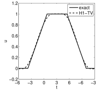
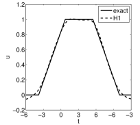
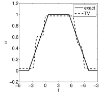
$u_{\mathrm{bdp}}$	$u_{\mathrm{h1}}$	$u_{\mathrm{tv}}$

Fig. 1: Numerical results for Example 1 with $\varepsilon=5\%$ noise.

The numerical results are summarized in Table 1. In the table, the subscripts $\mathrm{bdp}$ and $\mathrm{opt}$ respectively refer to the hybrid principle and the optimal choice, i.e., the value giving the smallest error. The single-parameter models are indicated by subscripts $\mathrm{h1}$ and $\mathrm{tv}$, and the regularization parameter shown in Table 1 is the optimal one. The accuracy of the results is measured by the relative $L^{2}$ error $e=\|u-u^{\dagger}\|_{\mathrm{L}^{2}}/\|u^{\dagger}\|_{\mathrm{L}^{2}}$. We observe that the $\mathrm{H}^{1}$-$\mathrm{TV}$ model in conjunction with the hybrid principle achieves a smaller error than either $\mathrm{H}^{1}$ or $\mathrm{TV}$ with the optimal choice, thereby showing the advantages of the $\mathrm{H}^{1}$-$\mathrm{TV}$ model. Further, the hybrid principle gives an error fairly close to the optimal one, within a factor of two, and the error decreases as the noise level decreases.

Let us briefly comment on the performance of the multi-parameter model. The classical $\mathrm{H}^{1}$ model recovers the flat region unsatisfactorily, whereas the $\mathrm{TV}$ approach clearly suffers from staircasing effect in the gray region and reduced magnitude in the flat region, cf. Fig. 1. In contrast, the $\mathrm{H}^{1}$-$\mathrm{TV}$ model preserves the magnitude of flat region while recovering the gray region excellently. Therefore, the $\mathrm{H}^{1}$-$\mathrm{TV}$ model does combine the strengths of both $\mathrm{H}^{1}$ and $\mathrm{TV}$ models. Finally, we would like to remark that Broyden’s method converges rapidly with the convergence achieved in five iterations, and the convergence behavior is not sensitive to the initial guess.

4.2 Elastic-net model

Example 2.

The kernel $k(s,t)$ is given by $\tfrac{1}{4}\left(\tfrac{1}{16}+(s-t)^{2}\right)^{-\frac{3}{2}}$, the exact solution $u^{\dagger}$ consists of two bumps and it is shown in Fig. 2. The penalties are $\psi_{1}(u)=\|u\|_{\ell^{1}}$ and $\psi_{2}(u)=\frac{1}{2}\|u\|_{\ell^{2}}^{2}$ to retrieve the groupwise sparsity structure, which is known as elastic-net in statistics [19]. The integration interval is $[0,1]$. The size of the problem is 100.

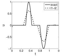
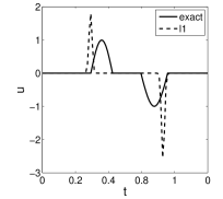
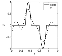
$u_{\mathrm{bdp}}$	$u_{\mathrm{l1}}$	$u_{\mathrm{l2}}$

Fig. 2: Numerical results for Example 2 with $\varepsilon=5\%$ noise.

Table 2: Numerical results for Example 2.

$\epsilon$	$\boldsymbol{\eta}_{\mathrm{bdp}}$	$\boldsymbol{\eta}_{\mathrm{opt}}$	$\eta_{\mathrm{l1}}$	$\eta_{\mathrm{l2}}$	$e_{\mathrm{bdp}}$	$e_{\mathrm{opt}}$	$e_{\mathrm{l1}}$	$e_{\mathrm{l2}}$
5e-2	(2.44e-3,9.60e-3)	(2.81e-3,1.16e-3)	1.16e0	3.11e-3	4.09e-1	8.57e-2	1.29e0	4.58e-1
5e-3	(7.30e-5,2.25e-4)	(2.59e-4,1.11e-4)	9.67e-5	3.13e-5	1.96e-1	1.20e-2	9.00e-1	2.90e-1
5e-4	(4.73e-6,1.27e-5)	(2.23e-5,1.11e-5)	1.27e-5	4.13e-6	7.50e-2	8.18e-3	6.18e-1	2.17e-1
5e-5	(3.29e-7,8.42e-7)	(2.73e-6,1.28e-6)	1.12e-6	3.79e-8	2.01e-2	4.69e-3	4.85e-1	1.66e-1
5e-6	(2.56e-8,6.50e-8)	(1.60e-7,9.92e-8)	5.14e-9	1.25e-9	1.16e-2	2.27e-3	2.62e-1	9.55e-2

It is observed from Table 2 that the hybrid principle gives slightly too small but otherwise reasonable estimate for the optimal choice. A close look at Fig. 2 indicates that the solution $u_{\mathrm{l2}}$ has almost no zero entries, and thus it fails to distinguish between relevant and irrelevant factors. Meanwhile, many entries of the $\ell^{1}$ solution are zero, and thus some relevant factors are correctly identified. However, it tends to select only a part instead of all relevant factors. The elastic-net combines the best of both $\ell^{1}$ and $\ell^{2}$ models, and it achieves the desired goal of identifying the group structure.

4.3 Image deblurring

Example 3.

The kernel $k(s,t)$ performs standard Gaussian blur with standard deviation $1$ and blurring width $5$. The exact solution $u^{\dagger}$ is shown in Fig. 3. The size of the image is $50\times 50$. The penalties are $\psi_{1}(u)=\|u\|_{\ell^{1}}$ and $\psi_{2}(u)=\frac{1}{2}\|u\|_{\ell^{2}}^{2}$.

$u^{\dagger}$	$u_{\mathrm{opt}}$
$u_{\mathrm{bdp}}$	$u_{\mathrm{l1}}$	$u_{\mathrm{l2}}$

Fig. 3: Numerical results for Example 3 with $\varepsilon=1\%$ noise. The selected regularization parameters are $\boldsymbol{\eta}_{\mathrm{bdp}}$=(4.70e-3,4.65e-3), $\boldsymbol{\eta}_{\mathrm{opt}}$ =(1.26e-2,1.31e-3), $\eta_{\mathrm{l1}}$=5.67e-1, and $\eta_{\mathrm{l2}}$=3.51e-3.

This example represents a more realistic problem of image deblurring. Here one half of the data points are retained, which renders the problem far more ill-posed. The $\ell^{1}$ solution is very spiky, cf. Fig. 3, and neighboring pixels act independently of each other. In particular, many pixels in the blocks and the cross are missing. In contrast, the solution $u_{\mathrm{l2}}$ is smooth, but there are many small spurious oscillations in the background. The elastic-net model achieves the best of the two: retaining the block structure with only few spurious nonzero coefficients. The numbers are also very telling: $e_{\mathrm{bdp}}=$2.96e-1, $e_{\mathrm{o}}$=2.44e-1, $e_{\mathrm{l1}}=$9.21e-1, and $e_{\mathrm{l2}}$=3.42e-1. Hence, the error $e_{\mathrm{bdp}}$ agrees well with the optimal choice, and it is smaller than that with the optimal choice for either $\ell^{1}$ or $\ell^{2}$ models.

5 Conclusions

We have studied multi-parameter regularization from the viewpoint of augmented Tikhonov regularization, and shown a unified way to derive the balancing principle and balanced discrepancy principle. A priori and a posteriori error estimates for the principles were provided, and efficient numerical algorithms (Broyden’s method and fixed point algorithm) were presented and discussed. Numerical results were presented to illustrate the feasibility of the balanced discrepancy principle.

References

- [1] M. Belge, M. E. Kilmer, and E. L. Miller. Efficient determination of multiple regularization parameters in a generalized L-curve framework. Inverse Problems, 18(4):1161–1183, 2002.
- [2] C. G. Broyden. A class of methods for solving nonlinear simultaneous equations. Math. Comp., 19(92):577–593, 1965.
- [3] M. Burger and S. Osher. Convergence rates of convex variational regularization. Inverse Problems, 20(5):1411–1420, 2004.
- [4] Z. Chen, Y. Lu, Y. Xu, and H. Yang. Multi-parameter Tikhonov regularization for linear ill-posed operator equations. J. Comput. Math., 26(1):37–55, 2008.
- [5] H. W. Engl, M. Hanke, and A. Neubauer. Regularization of Inverse Problems. Kluwer, Dordrecht, 1996.
- [6] B. Hofmann, B. Kaltenbacher, C. Poeschl, and O. Scherzer. A convergence rates result for Tikhonov regularization in Banach spaces with non-smooth operators. Inverse Problems, 23(3):987–1010, 2007.
- [7] K. Ito, B. Jin, and T. Takeuchi. Multi-parameter Tikhonov regularization. Methods Appl. Anal., 18(1):31–46, 2011.
- [8] K. Ito, B. Jin, and T. Takeuchi. A regularization parameter for nonsmooth Tikhonov regularization. SIAM J. Sci. Comput., 33(3):1415–1438, 2011.
- [9] K. Ito and K. Kunisch. BV-type regularization methods for convoluted objects with edge, flat and grey scales. Inverse Problems, 16(4):909–928, 2000.
- [10] V. K. Ivanov, V. V. Vasin, and V. P. Tanana. Theory of Linear Ill-Posed Problems and its Applications. VSP, Utrecht, second edition, 2002.
- [11] B. Jin and D. A. Lorenz. Heuristic parameter-choice rules for convex variational regularization based on error estimates. SIAM J. Numer. Anal., 48(3):1208–1229, 2010.
- [12] B. Jin and J. Zou. Augmented Tikhonov regularization. Inverse Problems, 25(2):025001, 25, 2009.
- [13] S. Lu and S. V. Pereverzev. Multi-parameter regularization and its numerical regularization. Numer. Math., 118(1):1–31, 2011.
- [14] S. Lu, S. V. Pereverzev, Y. Shao, and U. Tautenhahn. Discrepancy curves for multi-parameter regularization. J. Inv. Ill-Posed Probl., 18(6):655–676, 2010.
- [15] Y. Lu, L. Shen, and Y. Xu. Multi-parameter regularization methods for high-resolution image reconstruction with displacement errors. IEEE Trans. Circuits Syst. I. Regul. Pap., 54(8):1788–1799, 2007.
- [16] P. Mathé. The Lepskii principle revisited. Inverse Problems, 22(3):L11–L15, 2006.
- [17] I. M. Stephanakis. Regularized image restoration in multiresolution spaces. Opt. Eng., 36(6):1738–1744, 1997.
- [18] P. Xu, Y. Fukuda, and Y. Liu. Multiple parameter regularization: numerical solutions and applications to the determination of geopotential from precise satellite orbits. J. Geod., 80(1):17–27, 2006.
- [19] H. Zou and T. Hastie. Regularization and variable selection via the elastic net. J. R. Stat. Soc. Ser. B, 67(2):301–320, 2005.