Quantum non-Markovian behaviour at the chaos border

Abstract

In this work we study the non-Markovian behaviour of a qubit coupled to an environment in which the corresponding classical dynamics change from integrable to chaotic. We show that in the transition region, where the dynamics has both regular islands and chaotic areas, the average non-Markovian behaviour is enhanced to values even larger than in the regular regime. This effect can be related to the non-Markovian behaviour as a function of the the initial state of the environment, where maxima are attained at the regions dividing separate areas in classical phase space, particularly at the borders between chaotic and regular regions. Moreover, we show that the fluctuations of the fidelity of the environment – which determine the non-Markovianity measure – give a precise image of the classical phase portrait.

1 Introduction

The theoretical and experimental study of decoherence [1, 2] is important for – at least – two reasons. On the one hand to understand the emergence of classicality in the quantum framework. On the other hand, to assess and minimize the restrictions it imposes the development in new technologies being developed related to quantum information theory. Decoherence appears as the result of uncontrollable (and unavoidable) interaction between a quantum system and its environment. The expected effect is an exponential decay of quantum interference. Generally the theoretical approach is by means of a theory of open quantum systems [3]. The idea is to precisely divide the total system into system-of-interest plus environment and then discard the environment variables and derive en effective dynamical equation for the reduced system state. Obtaining and solving the effective equation is generally a very difficult task, so approximations are usually made. The Born-Markov approximation, which among other things assumes weak system-environment coupling and vanishing correlation times in the environment yields a Markov – memory-less – process, described by a semigroup of completely positive maps. The generator of these maps is given by the Lindblad-Gorini-Kossakowski-Sudarshan master equation [4, 5]. Lately, though, interest in problems where the Markov approximation is no longer valid have flourished (see [3, 6, 7, 8, 9, 10, 11, 12, 13], to name just a few). One very interesting feature of non-Markovian evolution is that information backflow can bring back coherence to the physical system and sometimes even preserve it [14, 15, 16].

Being able to quantify the deviation of markovianity (beyond a yes/no answer) is of importance to compare theory and experiment, specially in circumstances where the usual approximations (for example infinite size environment and weak coupling) start to break up. This leads to a proper understanding and the possibility to engineer non-Markovian quantum open systems which has many potential applications like quantum simulators [17], efficient control of entanglement [18, 19] and entanglement engineering [20], quantum metrology [21], or dissipation driven quantum information[22], and even quantum coherence in biological systems [23]. The simulation of non-Markovian dynamics and the transition from Markovian to non-Markovian has been recently reported in experiments [24, 25, 26].

There has been much activity in this context but one basic question remains untouched, namely that of the influence of the underlying classical dynamics of the environment on the central system. Intuition indicates that a chaotic environment should result in Markovian dynamics and a regular (or integrable) environment in strong non-Markovian effects. In [27] this transition has been studied. However, understanding the case where the environment has associated classical dynamics consisting of a mixture of regular islands, broken tori and hyperbolic dynamics, is still an open problem. The importance of this case is not to be overlooked being that mixed systems are the rule rather than the exception [28].

The purpose of this work is then to shed some light on the relation between the classical dynamics of the environment and its markovianity, for environments where the transition from regular to chaotic is tunable by a parameter. The complexities of such systems make analytical treatment almost impossible so we shall mainly focus on numerical simulations. In order to have access to some analytic results the central system will be the simplest possible. We center on a system consisting on a qubit coupled with an environment in a pure dephasing fashion. In such a way that the environment evolution is conditioned by the state of the qubit [29, 30, 31, 9, 32, 11, 27]. The qubit acts as a probe that can be used to extract important information from the dynamics of the environment [33]. As environment we use paradigmatic examples of quantum chaos: quantum maps on the torus. In particular we focus kicked maps which by changing one parameter one can go from integrable to chaotic.

To quantify non-Markovianity we use the measure proposed in [7] which is based on the idea of information flow, from and to the system. In our model this measure is directly related to the fidelity fluctuations of the environment. The time dependence of fidelity fluctuations can be used to extract important information about the dynamics of quantum chaotic systems, like the Lyapunov exponent [34]. For localized initial states the fidelity decay and fluctuations can be extremely state-dependent [35]. We found that the transition from integrable (“non-Markovian”) to chaotic (“Markovian”) is not uniform. In the transition there is a maximum which can be larger than the value that this measure attains for the regular dynamics. But more importantly, that the maximum happens at a value of the parameter that is critical in the corresponding classical dynamics, like the breakup of the last irrational torus, and the onset of unbound diffusion.

We show that the non-Markovian measure used reproduces the intricate structure of the classical phase space with extraordinary precision. Moreover, we observe that the values of non-Markovian measure as a function of position in phase space are enhanced in the regions that are neither chaotic nor regular, i.e. at the borders between chaos and regularity. This establishes the non-Markovianity measure used, which depends on the long time fidelity fluctuations, as pointer to the chaos border. Another way of identifying this border can be found in [36]. As a consequence, our results contribute to a deeper understanding of the fidelity decay of quantum systems with mixed classical dynamics, which is an open problem of current interest [37, 38, 39].

This paper is organized as follows. In Sec. II we introduce the definition and the measure of non-Markovianity that we use throughout the paper. Then in Sect III we describe the way that our model environment interacts with the central system which is a qubit. We explicitly write the dynamical map and show how the non-Markovianity measure we chose to use depends on the fidelity of the environment. In Sec. IV we give a brief description of the quantum maps that we use a model environments. Depending on a parameter the corresponding classical dynamics of these maps can go from integrable to chaotic. In sections V and VI we show numerical results. In Sec. V for the environment in a maximally mixed state. In Sec. VI for the environment initially in a pure state. On average both cases show qualitatively similar results. In addition in Sec. VI we show how the classical phase space structure is obtained when the non-Markovianity measure is plotted as a function of the initial state. We draw our conclusions in Sec. VII and we include an appendix where we explain some technical details of the short time behaviour of the fidelity decay.

2 Measuring Non-Markovianity: information flow

The notion of Markovian evolution, both classical and quantum is associated with an evolution in which memory effects are negligible. In classical mechanics this is well defined in terms of multiple-point probability distributions. In quantum mechanics evolution of an open system is often assumed to be well described by a Lindblad master equation (which can also be credited to Gorini, Kossakowski and Sudarshan [4, 5]). The Lindblad master equation generates a one parameter family of completely positive, trace preserving (CPT) dynamical maps, also called quantum dynamical semigroup. The semigroup property implies lack of memory. But the validity of the Lindblad master equation description relies heavily on the Born-Markov approximation, and other restrictions. Unfortunately there are many cases in which these approximations do not apply, especially when weak coupling is no longer valid, but also in the case of finite environments. One of the key issues is to consistently define and quantify non-Markovian behaviour for quantum open systems. Recently there have been some attempts to define and quantify non-Markovianity (some of them are reviewed in [40]). One of these attempts is based on the fact that Markovian systems contract, with respect to the distance induced by the norm-1, the probability space [41]. This is often interpreted as an information leak from the system into an environment, as one decreases with time the ability to infer the initial condition from the state at a given time. The very same idea has been used in quantum systems. Distinguishability between quantum states is quantified with the trace norm [42], and whenever this quantity increases with time is interpreted as a measure of non-Markovian beahvior in the quantum system by Breuer, Laine and Piilo (BLP) in [7]. As this quantity is related to an information flow, and is simple in our case to calculate, we are going to use it to quantify non-Markovianity.

The first step is to define a way to distinguish two states. We do that by means of the trace distance. Given two arbitrary states represented by their density matrices $\rho_{1}$ and $\rho_{2}$ the trace distance is defined by

$$D(\rho_{1},\rho_{2})=\frac{1}{2}{\rm Tr}|\rho_{1}-\rho_{2}|.$$ (1)

It is a well defined distance measure with all the desired properties and it can be shown to be a good measure of distinguishability [43]. Another property of the trace distance is that

$$D(U\rho_{1}U^{\dagger},U\rho_{2}U^{\dagger})=D(\rho_{1},\rho_{2})$$ (2)

i.e. it is invariant under unitary transformations and is a contraction

$$D(\Lambda\rho_{1},\Lambda\rho_{2})\leq D(\rho_{1},\rho_{2})$$ (3)

for any CPT quantum channel $\Lambda$. Thus no CPT quantum operation can increase distinguishability between quantum states. The idea proposed by BLP is that under Markovian dynamics the information flows in one direction (from system to environment) and two initial states become increasingly indistinguishable. Information flowing back to the system would allow for memory effects to manifest. A process is then defined to be non-Markovian if at a certain time the distance between to states increases, or

$$\sigma(t,\rho_{1.2}(0))\equiv\frac{d}{dt}D(\rho_{1}(t),\rho_{2}(t))>0.$$ (4)

With this in mind non-Markovian behaviour can be quantified by [7]

$${\cal M}=\max_{\rho_{1,2}(0)}\int_{\sigma>0}dt\sigma(t,\rho_{1.2}(0)),$$ (5)

i.e. the measure of the total increase of distinguishability over time. The maximum is taken over all possible pairs of initial states.

We should remark here that there are many other proposed measures. Rivas, Huelga and Plenio (RHP) [8] proposed two measures which are based on the evolution of entanglement to an ancilla, under trace preserving completely positive maps. There are others based on Fisher information [44] or the validity of the semigroup property [45]. For some situations [46] BLP and RHP are equivalent. In our case, it is easy to see that the RHP measure, which relies on monotonous decay of entanglement in Markovian processes, differs from the BLP measure by a constant factor. So in the present work we only consider BLP.

3 Non-Markovianity and fidelity fluctuations

We assume that the interaction between the environment and the probe qubit is factorizable, and that it commutes with the internal hamiltonian of the qubit. Neglecting the qubit Hamiltonian, by selecting the appropriate picture, and choosing a convenient basis, one can write the Hamiltonian as

$$H=\mathbbm{I}\otimes H_{\rm env}+\delta\sigma_{z}\otimes V.$$ (6)

Properly rearranged, one can write the hamiltonian of the form

$$H=|0\rangle\!\langle 0|\otimes H_{0}+|1\rangle\!\langle 1|\otimes H_{1},$$ (7)

were $H_{0}$ and $H_{1}$ act only on the environment and $|0\rangle\!\langle 0|$, $|1\rangle\!\langle 1|$ are projectors onto some orthonormal basis of the qubit [29]. In this case, the coupling $\delta V=(H_{0}-H_{1})/2$ is given by the difference of the hamiltonians of the environment in Eq. (7). This kind of pure dephasing interactions occur spontaneously in several experiments (for example [47]), but can also be engineered [48, 32].

We suppose that initially system and environment are not correlated, which can be expressed as $\rho_{{\rm sys},\text{env}}(0)=\rho_{\rm sys}(0)\otimes\rho_{\text{env}}$. To focus only on the system, the environment degrees of freedom should be traced out

$$\rho_{\rm sys}(t)={\rm Tr}_{\text{env}}\left[U(t)\rho_{\rm sys}(0)\otimes\rho_{\text{env}}U^{\dagger}(t)\right]$$ (8)

with

$$U(t)=|0\rangle\!\langle 0|U_{0}(t)+|1\rangle\!\langle 1|U_{1}(t).$$ (9)

This yields a dynamical map for the qubit that we write as

$$\rho_{\rm sys}(t)=\Lambda(t)(\rho_{\rm sys}(0))$$ (10)

which, in the basis of Pauli matrices, takes the form

$$\Lambda=\begin{pmatrix}1&0&0&0\\ 0&{\rm Re}[f(t)]&{\rm Im}[f(t)]&0\\ 0&{\rm Im}[f(t)]&{\rm Re}[f(t)]&0\\ 0&0&0&1\end{pmatrix}.$$ (11)

Here we have taken conventionally $\{\sigma_{i}\}=\{\mathbb{I},\sigma_{x},\sigma_{y},\sigma_{z}\}$ and $\Lambda_{j,k}=(1/2){\rm Tr}\left[\sigma_{j}U(t)\sigma_{k}\otimes\rho_{\rm env}U^{\dagger}(t)\right]$. In Eq. (11) $f(t)={\rm Tr}[\rho_{\rm env}U_{1}(t)^{\dagger}U_{0}(t)]$ is the expectation value of the echo operator $U_{1}(t)^{\dagger}U_{0}(t)$ . In this work we will assume that $H_{1}$ ($U_{1}$) is just a perturbation of $H_{0}$ ($U_{0}$). If $\rho_{\text{env}}$ is pure then $|f(t)|^{2}$ is the well known quantity called Loschmidt echo [49] – also called fidelity – which can be used to characterize quantum chaos [37, 38, 39]

In our case, where the system is one qubit, the states that maximize ${\cal M}$ in Eq. (5) are pure orthogonal states lying at the equatorial plane on the Bloch sphere. [50]. Here we consider two cases. If the state of the environment is a pure state [11] $\rho_{\text{env}}=|\psi\rangle\!\langle\psi|$ then we get

$${\cal M}_{\rm p}(t) = 2\int_{t=0,\dot{|f|}>0}^{t}d\tau\frac{d|f(\tau)|}{d\tau}$$ (12)

$$\equiv 2\sum_{i}[|f(t_{i}^{(\rm max)})|-|f(t_{i}^{(\rm min)})|].$$

where $|f(t)|=|{\langle\psi|}U_{1}^{\dagger}(t)U_{0}(t){|\psi\rangle}|$ is the square root of the Loschmidt echo and $t_{i}^{(\rm max)}>t_{i}^{(\rm min)}$ correspond to the times of successive local maxima and minima of $|f(t)|$. ${\cal M}_{p}$ is the quantity considered in [11]. Throughout the paper, when the initial state is pure we will consider a coherent state centered at some point $(q,p)$ to be defined.

On the other hand, if we have no knowledge or control over the environment, then it will most likely be in a mixed state. If we assume it is in a maximally mixed state $\rho_{\rm env}=I/N$ (with $I$ the identity in the Hilbert space of the environment) we get [27]

$${\cal M}_{\rm m}(t)=2\sum_{i}[|\langle f(t_{i}^{(\rm max)})\rangle|-|\langle f(t_{i}^{(\rm min)})\rangle|],$$ (13)

where $\langle f(t)\rangle$ is the average fidelity amplitude. If the average is done over a complete set of states then

$$\langle f(t)\rangle=\frac{1}{N}{\rm tr}[U_{1}^{\dagger}(t)U_{0}(t)]$$ (14)

which depends only on the set of states being complete, but not on the kind of states.

In the results that we present we model the dynamics of the environment $U_{0,1}$ using quantum maps on the torus with a finite Hilbert space. Here, one can write Eq. (9) as

$$U=\begin{pmatrix}U_{0}&0\\ 0&U_{0}\end{pmatrix}\begin{pmatrix}\mathbbm{I}&0\\ 0&U_{0}^{\dagger}U_{1}\end{pmatrix}$$ (15)

so the coupling is provided by the echo operator $U_{0}^{\dagger}U_{1}$. In this case, after some time the fidelity fluctuates around some constant value. This causes a linear growth with time of ${\cal M}_{\rm p}$ and ${\cal M}_{\rm m}$ (the slope goes to zero with the size of the Hilbert space). For this reason we follow the strategy of [27] and consider ${\cal M}_{\rm m}$ and ${\cal M}_{\rm p}$ up to some finite time $t$.

4 Kicked maps

For the numerical simulations we suppose that the dynamics of the environment is given by a quantum map on the torus. Apart from the fact that these maps are the simplest paradigmatic examples of quantum chaotic dynamics, the ones we consider can be very efficiently implemented using fast Fourier transform. Due to periodic boundary conditions the Hilbert space is discrete and of dimension $N$. This defines an effective Planck constant $\hbar=1/(2\pi N)$. Position states can be represented as vertical strips of width $1/N$ at positions $q_{i}=i/N$(with $i=0,\,\ldots,\,N-1$) and momentum states are obtained by discrete Fourier transform. A quantum map is simply a unitary $U$ acting on an $N$ dimensional Hilbert space. Quantum maps can be interpreted as quantum algorithms and vice-versa. In fact there exist efficient – i.e. better than classical – quantum algorithms for many of the well known quantum maps [51, 52, 53, 54, 55, 56], making them interesting testbeds of quantum chaos in experiments using quantum simulators (e.g. [54, 57, 32]).

Here we consider two well known maps with the characteristic properties of kicked systems, i.e. they can be expressed as

$$U=T(\hat{p})V(\hat{q}).$$ (16)

They also share the property that by changing one parameter (the kicking strength) they can be tuned to go from classical integrable to chaotic dynamics.

The quantum (Chirikov) standard map (SM) [58]

$$U_{K}^{({\rm SM})}=e^{-i\frac{{\hat{p}}^{2}}{2\hbar}}e^{-i\frac{K}{\hbar}\cos(2\pi\hat{x})}$$ (17)

corresponds to the classical map

$$\begin{array}[]{lll}p_{n+1}&=&p_{n}+\frac{K}{2\pi}\sin(2\pi x_{n})\\ x_{n+1}&=&x_{n}+p_{n+1}.\end{array}$$ (18)

Since we consider a toroidal phase space both equations are to be taken modulo 1. For small $K$ dynamics is regular. Below a certain critical value $K_{c}$ the motion in momentum is limited by KAM curves. These are invariant curves with irrational frequency ratio (or winding number) which represent quasi-periodic motion, and they are the most robust orbits under nonlinear perturbations[59]. At $K_{c}=0.971635\ldots$ [60], the last KAM curve, with most irrational winding number, breaks. Above $K_{c}$ there is unbounded diffusion in $p$. For very large $K$, there exist islands but the motion is essentially chaotic.

The quantum kicked Harper map (HM)

$$U^{({\rm HM})}_{K_{1},K_{2}}=e^{-i\frac{K_{2}}{\hbar}\cos(2\pi\hat{p})}e^{-i\frac{K_{1}}{\hbar}\cos(2\pi\hat{x})}$$ (19)

is an approximation of the motion of kicked charge under the action of an external magnetic field [61, 62]. Equation (19) corresponds to the classical map

$$\begin{array}[]{lll}p_{n+1}&=&p_{n}-K_{1}\sin(2\pi x_{n})\\ x_{n+1}&=&x_{n}+K_{2}\sin(2\pi p_{n+1})\end{array}$$ (20)

From now on, unless stated otherwise we consider $K_{1}=K_{2}=K$.” For $K<0.11$, the dynamics described by the associated classical map is regular, while for $K>0.63$ there are no remaining visible regular islands [63].

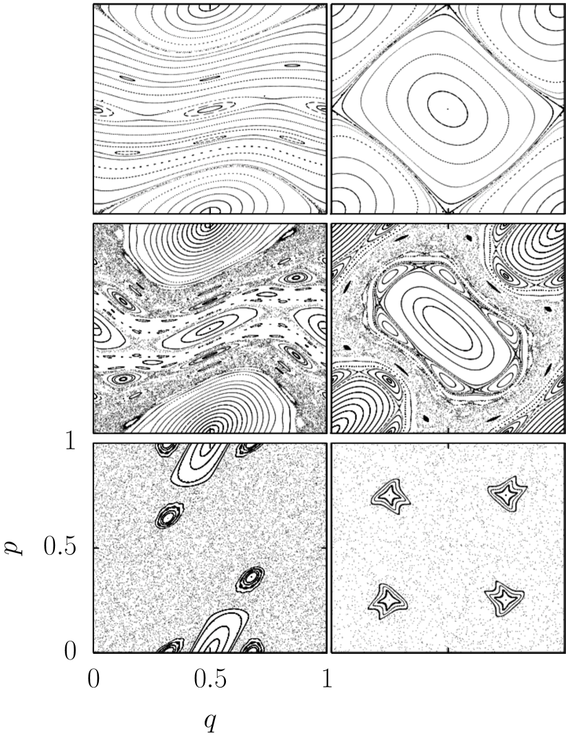
Figure 1: Phase space portrait for the classical SM (left column) and the HM, with $K_{1}=K_{2}=K$ (right column) for different values of $K$. (top, left) $K=0.5$, (top, right) $K=0.1$; (center left) $K=0.98$, (center, left) $K=0.25$; (bottom left) $K=2.5$, (bottom right) $K=0.5$

In Fig. 1 we show examples of phase space portraits for the two maps for three different values of $K$ where the transition from regular to mainly chaotic can be observed.

For the numerical calculations we take for the standard map $U_{0}\equiv U_{K}^{({\rm SM})}$ and $U_{1}\equiv U_{K+\delta K}^{({\rm SM})}$ and for the Harper map $U_{0}\equiv U^{({\rm HM})}_{K,K}$ and $U_{1}\equiv U^{({\rm HM})}_{K,K+\delta K}$. So $\delta K$ is the perturbation strength.

5 Non-Markovianity at the frontier between chaos and integrability

Both the SM and the HM offer the opportunity to explore the transition form integrability to chaos by changing the kicking parameter. By doing that (for the HM) two things were found in [27]. As expected, For very large $K$, which corresponds to chaotic dynamics, Markovian behaviour was observed. On the other hand, for small $K$ corresponding to regular dynamics, non-Markovian behaviour was obtained.

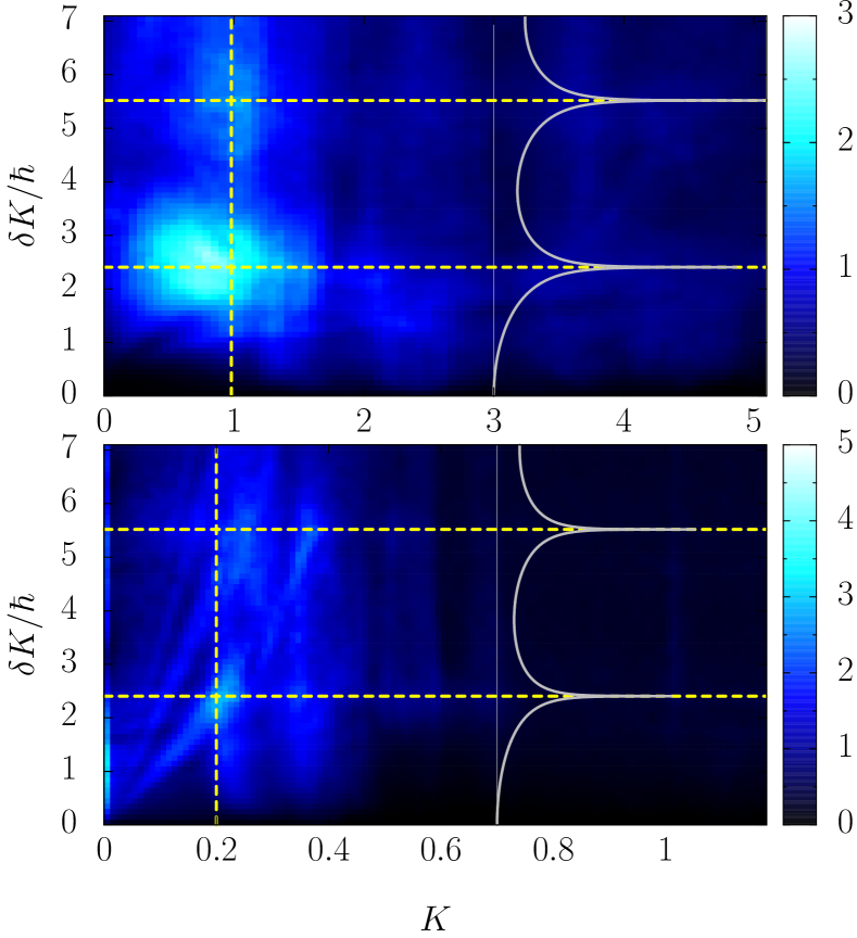
Figure 2: ${\cal M}(t=200)$ as a function of $K$ (varying the dynamics of the environment) and $\delta K/\hbar$ (controlling the coupling strength) for the quantum standard (top) and the quantum Harper map (bottom) with $N=500$. The vertical lines are (top) $K=0.98\approx K_{c}$, and (bottom) $K=0.2$. Horizontal dashed lines mark is the first values of $\delta K$ such that $J_{0}(\delta K/\hbar)=0$. Overlay (gray/solid) curves correspond to $\Gamma(\delta K/\hbar)$ from Eq. (22), rescaled to fit in the plot.

However, there was an unexpected result: the transition is not uniform. There is a clear peak in ${\cal M}_{\rm m}(t)$ – Fig. 3 in [27] – that, depending on the value of $\delta K$ and $t$ can even be larger than the value for regular dynamics. To complement this previous result and further illustrate this effect we calculated ${\cal M}_{\rm m}(t)$ as a function of $K$ and $\delta K$. In particular, for very short times, the decay of the fidelity amplitude has a rich structure [64]. It can be shown by semiclassical calculations that for short times the decay of the average fidelity amplitude is given by

$$|\langle f(t)\rangle|\sim e^{-\Gamma t}.$$ (21)

The decay rate gamma can be computed semiclassically [64] and Eq. (21) is valid for increasingly larger times as the system becomes more chaotic. For $t=1$, in the case of the HM and the SM, $\Gamma$ can be computed analytically (see appendix) and it is given by

$$\Gamma=-\ln|J_{0}(\delta K/\hbar)|,$$ (22)

where $J_{0}$ is the Bessel function. Thus when $J_{0}(\delta K/\hbar)=0$, $\Gamma$ diverges. It can be observed that in fact this is the case. The fidelity amplitude decays very fast for short times, and then there is a strong revival which translates in an increase of ${\cal M}_{\rm m}$ [27].

In Fig. 2 we show ${\cal M}_{\rm m}(t=200)$ for the SM (top) and the Harper map (bottom). The horizontal axis is the kicking strength $K$ and vertical axis is the rescaled perturbation $\delta K/\hbar$. In both cases there are clearly distinguishable maxima. The horizontal dashed lines mark the points where $\Gamma$ diverges, which is seen in the overlay plot of $\Gamma(\delta K/\hbar)$ (solid/gray lines). As expected, along those lines ${\cal M}_{\rm m}$ is larger due to a large revival of the fidelity amplitude for small times.

The dashed vertical line, on the other hand, marks the position of the peak on the $K$ axis. For the SM we placed the line on the value $K_{\rm c}\approx 0.98$ were the transition to unbound diffusion takes place. For the kick Harper map with $K_{1}=K_{2}$ there is no analog transition, however we see a peak near $K=0.2$.

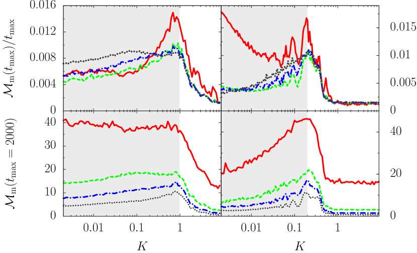
Figure 3: Top row: ${\cal M}_{\rm m}(t_{\rm max})/t_{\rm max}$ as a function of the kicking strength $K$ with $N=512$ , for different times $t_{\rm max}=100$(solid/red), $500$ (dash/green), $1000$ (dot-dash/blue), $4000$ (dot/gray) for (Left) SM. (Right) HM. Bottom row: ${\cal M}_{\rm m}(t_{\rm max}=2000)$ as a function of $K$, for different environment sizes $N=100$ (solid/red), $N=500$ (dash/green), $N=1000$ (dot-dash/blue), and $N=2000$ (dot/gray) for (Left) SM and (Right) HM. In all cases $\delta K/\hbar=2.0$

In Fig 3 we show ${\cal M}_{\rm m}(t)$ as a function of $K$ for the case $\delta K/\hbar=2.0$. Panels on the left (right) correspond to the SM (HM). On the top we consider the dependence with time. It is clear that for a fixed dimension $N$, as time increases the peak establishes at a fixed value. The good scaling with $t_{\rm max}$ (after the peak) can be explained as follows: as the environment becomes more chaotic, the fidelity decays faster and fluctuates around a constant value. As a consequence, the growth of ${\cal M}_{\rm m}(t)$ becomes linear in time – much sooner for a chaotic environment –, with a slope proportional to ($1/N$) [27]. So for a fixed $N$, the curves should scale with time. The discrepancy for short $t$ is understood because the linear regime is not yet attained. On the bottom row of Fig 3 we explore the possibility of finite size effects. We show ${\cal M}_{\rm m}(t=2000)$ with a fixed $t$. As $N$ grows the peak settles at a constant value – again $K\approx 0.98$ for the SM and $K\approx 0.2$ for the HM (both marked by the limit of the shaded region).

We conclude this section by stating that ${\cal M}_{\rm m}(t)$, which depends on the fluctuations of the average fidelity amplitude, seems to be reinforced at a classically significant point in parameter space for the SM, namely $K_{c}$. On the other hand for the HM we make a complementary remark. Since the peak at $K=0.2$ seems to be robust (both changing $N$ and $t_{\rm max}$, we conjecture that in analogy to $K_{c}$ of the SM there should be a similar transition, at least in some global property of the classical map, near $K=0.2$. We postpone that discussion until Sec. 6.3.

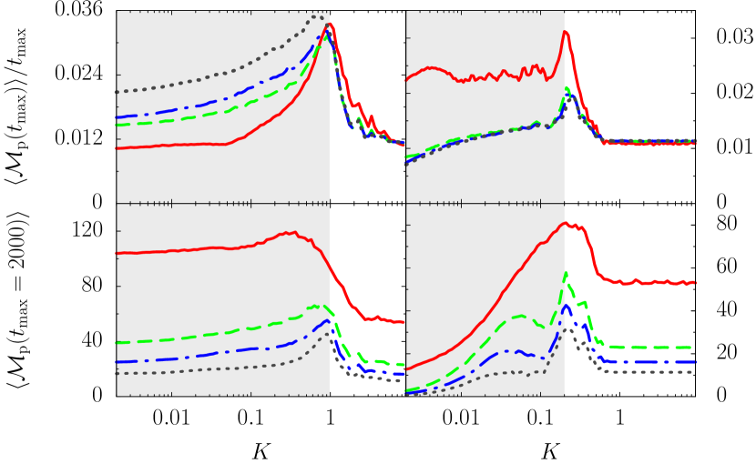
Figure 4: Same as Fig. 3 for ${\cal M}_{\rm p}(t)$

6 Environment in a pure state: classical phase space revealed

In the previous section we obtained unintuitive results for the non-Markovianity when the dynamics of the environment goes from integrable to chaotic. In particular there appears to be maxima of ${\cal M}_{\rm m}$ as a function of $K$ (and $\delta K$). To obtain these results, we chose the initial state of the environment to be in a maximally mixed state so the measure ${\cal M}_{\rm m}(t)$ depends on the average fidelity amplitude (see Eq. (13)). This average is a sum of amplitudes and interference effects could be argued to be at the origin of the peaks observed. For completeness, in this section we suppose the environment to be initially in a pure state [11], in particular a Gaussian – or coherent – state, using ${\cal M}_{\rm p}(t)$ of Eq. (12), for two reasons. First to contrast the global properties obtained with ${\cal M}_{\rm m}(t)$ , through the average behaviour of the fidelity. But also, to show that ${\cal M}_{\rm p}(t)$, and as a consequence fidelity fluctuations, as a function of the center of the initial Gaussian wave packet, gives a precise image of the classical phase portrait.

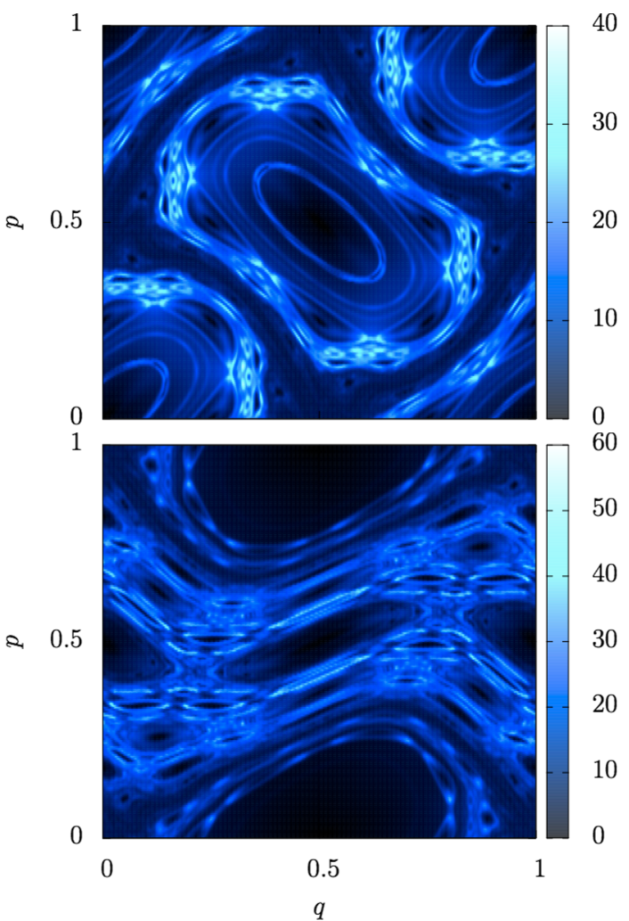
Figure 5: ${\cal M}_{\rm p}(t)$ as a function of the center $(q_{0},p_{0})$ of the initial Gaussian wave packet with $N=5000$, $\delta K/\hbar=2$ and $t=500$ for the SM with $K=0.98$ (bottom) and the HM with $K=0.25$ (top).

6.1 Correspondence between ${\cal M}_{\rm m}$ and $\langle{\cal M}_{\rm p}\rangle$

In this section we contrast the results for ${\cal M}_{\rm m}(t)$ in Sec. 5 with the ones for the average of ${\cal M}_{\rm p}(t)$. We consider a uniform grid of $N$ points at positions $q_{i}=i/\sqrt{N},\,p_{j}=j/\sqrt{N}$ and place coherent state centered at each pair $q_{i},p_{j}$. We then average over all the initial states of the environment and get

$$\langle{\cal M}_{\rm p}(t)\rangle=\frac{1}{N}\sum_{i=0}^{\sqrt{N}-1}\sum_{j=0}^{\sqrt{N}-1}{\cal M}_{\rm p}^{(q_{i},p_{j})}(t),$$ (23)

where ${\cal M}_{\rm p}^{(q_{i},p_{j})}(t)$ is just ${\cal M}_{\rm p}(t)$ for a particular Gaussian state centered at $(q_{i},p_{j})$.

In Fig. 4 we show for $\langle{\cal M}_{\rm p}(t)\rangle$ the curves for the parameters that correspond to the ones obtained in Fig. 3. As expected, the curves are different, but the qualitative properties are very similar. Mainly the marked peak at $K\approx 0.98$ for the SM and at $K\approx 0.2$ for the HM are preserved. On the top row, we observe that after the peak the scaling with $t_{\rm max}$ also holds. On the bottom row the dependence with $N$ is shown. It is also clear that the peak becomes more defined as $N$ grows.

6.2 Classical phase space sampling using ${\cal M}_{\rm p}$

We have shown (Figs. 3 and 4) that qualitatively there is no difference between the non-Markovianity for the environment in a completely mixed state and the average non-Markovianity for the environment in a pure coherent state. This is what we called global feature, “global” referring to an average over states covering the whole phase space. The only difference is whether we do the average over amplitudes (${\cal M}_{\rm m}$) or probabilities (${\cal M}_{\rm p}$) . Nevertheless for individual pure states of the environment, non-Markovianity is strongly state-dependent. In this section we seek to show this dependence is strongly related to the details of the classical phase space portrait of the environment. For this, we again define a grid of $n_{s}$ points $q_{i},\,p_{j}=0,1/\sqrt{n_{s}},\ldots,(\sqrt{n_{s}}-1)/\sqrt{n_{s}}$. We then compute ${\cal M}_{\rm p}(t)$ for a fixed time, and we plot this as a function of initial position and momentum. In other words we plot ${\cal M}_{\rm p}^{(q_{i},p_{j})}(t)$ from Eq. (23). The results obtained were surprising. We did expect that the classical dynamics should and would have some kind of effect. However we did not expect that ${\cal M}_{\rm p}$ would reproduce with such detail the complexities of the classical phase space. In Fig. 5 it is shown how all the classical structures are very well reproduced by the landscape built from ${\cal M}_{\rm p}(t)$ as a function of $q_{i}$ and $p_{j}$ (see the corresponding classical cases in Fig. 1). Of course, the ability to resolve classical structure will be limited by two factors: the dimension $N$ (or equivalently, size of effective $\hbar$), and the number of initial states $n_{s}$ (or “pixels”). In Fig. 5 it could be argued that $N=5000$ is almost classical. This argument becomes relative when one considers that a quantum map with $N\approx 5000$ could be implemented in a quantum computer of the order of, a little more than, 12 qubits (not a very big number of particles).

But the most surprising thing is that, contrary to intuition, ${\cal M}_{\rm p}(t)$ is almost as small for a regular environment (i.e. when the initial state is localized inside a regular island) as for chaotic a chaotic environment. On the contrary ${\cal M}_{\rm p}(t)$ exhibits peaks at the regions that separate different types of dynamics. Specifically at the complex areas consisting of broken tori that separate regular islands and chaotic regions and near hyperbolic periodic points. This means that the main contribution to the average non-Markovianity (in the mixed phase space case) does not come form the regular parts. In Fig. 6 we show a two dimensional curve that corresponds to a detail of the HM case in Fig. 5. Two things can be directly observed. The first one is how ${\cal M}_{\rm p}$ becomes larger and has maxima in the regions that lie between regular and chaotic behavior. But also how larger $N$ resolve better the small structures. In particular elliptic periodic points are expected to be a minimum of ${\cal M}_{\rm p}$ because they are structurally stable and so a small perturbation leaves them unchanged. In that case fidelity does not decay, or decays very slowly. The dashed (blue) line ($N=1000$) detects the change between regular and chaotic, but does not resolve the structure inside the island. In this case the width of a coherent state ($1/\sqrt{N}$) is of the order, or larger, than the size of the island. On the contrary, for larger $N$ (red line) the structure inside the island is well resolved and ${\cal M}_{\rm p}$ has maxima on the borders of the island and is minimal on top of the periodic point.

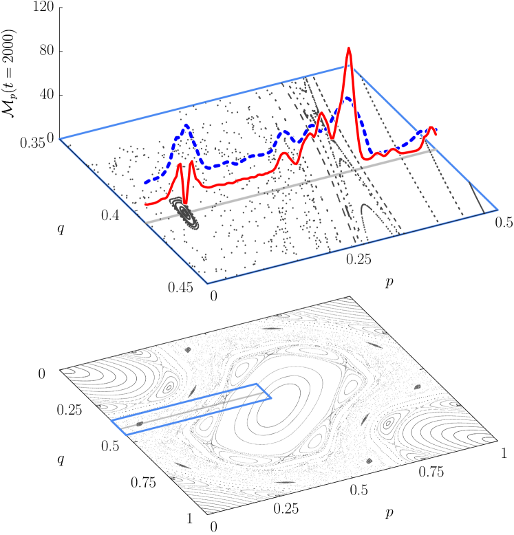
Figure 6: ${\cal M}_{\rm p}(t=2000)$ as a function of initial position ($q_{0}=0.408171$, $p_{0}\in[0,0.5]$) of the state of the environment and two different dimensions (red/solid) $N=4000$, (blue/dashed) $N=1000$. The map is the quantum HM with $K=0.25$, $\delta K/\hbar=2$. The blue square on the bottom indicates the area that is detailed above.

It is worth pointing out, that non-Markoviantiy in the regular and chaotic regions have very different scaling with $N$. For a fixed, large time – $t\sim 2000$ – we have observed that in the chaotic region ${\cal M}_{\rm p}$ decays as $1/\sqrt{N}$, while in the regular region ${\cal M}_{\rm p}$ grows as $\sqrt{N}$ (we have observed this numerically for sizes up to $N=6\times 10^{5}$). In the border regions, the behaviour has no clear scaling with $N$, as the small classical structures are better resolved.

A further comment on the finite-size scaling: it is known that finite N in a quantum map implies that at some point in time recurrences occur. Build-ups in fidelity can be observed at around Heisenberg time ($T_{\rm H}\approx N$)[65]. The contribution of these isolated revivals are negligible as opposed to the very frequent revivals that occur for systems in the border regions (see Fig. 8). In fact, in the semiclassical limit ($N\to\infty$) these Heisenberg time revival looses all meaning.

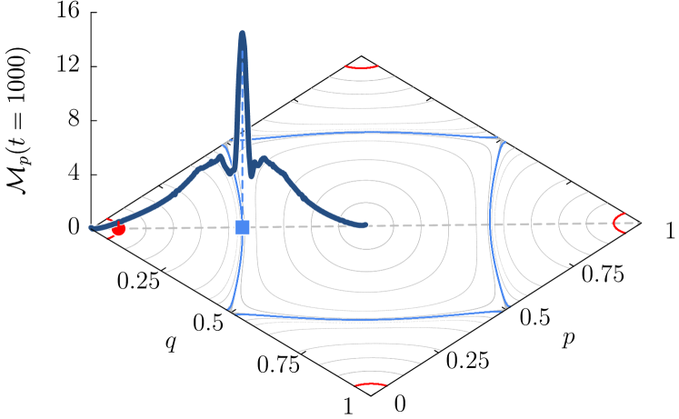
Figure 7: ${\cal M}_{\rm p}(t=1000)$ as a function of the position $q_{0}=p_{0}$ of the initial state of the environment. The map is the quantum HM with $N=2000$, $K=0.1$, $\delta K/\hbar=2$. Dark lines are the classical trajectories corresponding to the to curves shown in Fig. 8.

From the numerical results we conclude that the main contribution to non-Markovian behaviour comes from the regions of phase space that delimit two separate regions – like chaotic and regular regions, and also two disjoint regular islands. The relation with the fidelity is key to understanding this effect. For states in the chaotic region the fidelity decays exponentially and saturates at a value which depends on the size of the chaotic area (typically proportional of order $1/N$). The main contribution to non-Markovianity for chaotic initial conditions come from small time revivals (see e.g. [64]). The contribution due to fluctuations around the saturation value grows linearly with time, but with a slope that is inversely proportional to $N$, so in the large $N$ limit it can be neglected. Gaussian initial states inside regular islands evolve in time with very small deformation, so the fidelity is expected to decay very slowly and eventually there will be very large (close to 1) revivals. However the large revivals will be sparse and their contribution to non-Markovianity will be small. In the border areas there is no exponential spreading so the initial decay is be slower, and there is no chaotic region so there is no expected saturation. As a result after a short time decay we observe numerically that there are high frequency fluctuations that contribute strongly to the non- Markovianity measure.

We illustrate this in Figs. 7 and 8 . In Fig. 7 we show ${\cal M}_{\rm p}(t=1000)$ for the HM with coherent states centered at $q=p$. There is a minimum at the fixed point which is understood again in terms of structural stability: when the map is perturbed, the fixed point remains a fixed point, so fidelity does not decay. To further understand we use Fig.  8 where we show the fidelity and ${\cal M}_{\rm p}(t)$ for the two points marked in Fig.  7 (circle: $q_{0}=p_{0}=0.05$; square: $q_{0}=p_{0}=0.275$). Inside the islands the motion of the wave packets is more or less classical with little stretching over long times. Fidelity decays slowly and since there is practically no deformation, there are large revivals at times of the order of $N$ (solid/red curve in Fig. 8 top). On the contrary at the separatrix the wave packets spread and though initially fidelity decays fast, there remains a significant overlap the whole time. The complex motion accounts for the fluctuations (dashed/blue curve in Fig. 8 top) and the resulting maximum of ${\cal M}_{\rm p}$ seen in Fig .7.

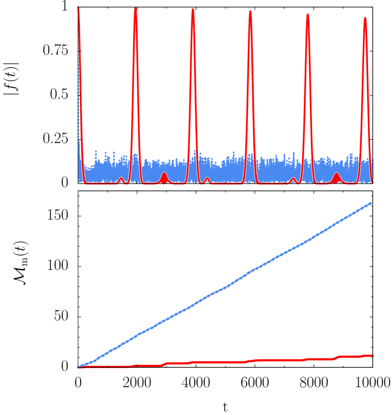
Figure 8: Top: $|f(t)|$ for two coherent states evolved with the quantum HM for $K=0.1$, $\delta K/\hbar=2.0$ and $N=2000$. (blue) $q_{0}=p_{0}=0.275$ corresponds to the maximum seen in Fig. 7, and (red) $q_{0}=p_{0}=0.05$.

A deeper understanding of the behaviour of the non Markovianity measure ${\cal M}(t)$ at the border between the chaotic and integrable region would be desirable. We have observed that in that region, for long times, the wave function is trapped within a relatively small portion of phase space. We could infer that, for these times, there is going to be a smaller area of phase space available, and the wave function will behave approximately randomly with time. The smaller phase space available, translates into a smaller effective Hilbert space, where the fluctuations will thus be larger. To support this reasoning we have observed that both the Husimi and Wigner (without ghost images [66]) functions of states contributing largely to the measure of non-Markovianity remain localized inside the sticky area near the KAM region [67, 68]. We also tested if the Fourier transformation of the fidelity amplitude is compatible with random data (i.e. has little or no structure). Moreover, we looked at the distribution of fidelity amplitude, which if it had Gaussian distribution it would be compatible with the inner product of two random state. However, although we have found that the distribution of the fluctuations of the fidelity amplitude is indeed Gaussian for many cases, the Fourier transform at the border exhibits some clear peaks meaning that the behaviour is not completely random, so it is not simply a matter of smaller effective Hilbert space dimension. Work in this direction is in progress.

6.3 Compatibility with classical results

The results obtained in the previous sections relate NM with some global property of the classical system. For the standard map there is a critical value $K_{\rm c}$ of the kicking strength after which the motion in the momentum direction (when the map is taken in the cylinder) becomes unbounded. This value, estimated to be $K_{\rm c}=0.971635\ldots$ [60], corresponds to the breaking of the torus with most irrational winding number.

Motion for the kicked Harper map on the contrary is different. For $K=0$ it is integrable with a separatrix joining the unstable fixed points $(0,1/2),\,(1/2,0),\,(1,1/2),\,(1/2,1)$. For $K>0$ the separatrix breaks and – if considered on the whole plane – a mesh of finite width forms, also called stochastic web. Motion inside this mesh is chaotic and diffusion is unbounded for all $K$.

Although –to our knowledge – for the HM there is no critical $K$ analog to $K_{\rm c}$ for the standard map, the peaks in Figs. 2, 3, and 4 hint that there could exist a similar kind of transition function of $K$. To test this conjecture we evaluate two different global quantities. First we take into account diffusion. Considering the map on the whole plane (i.e. no periodic boundaries) if diffusion is normal then the spreading, e.g. in momentum, should grow linearly with time (number of kicks). Thus we define

$$D=\lim_{t\to\infty}\frac{\langle(p_{t}-p_{0})^{2}\rangle}{t},$$ (24)

where the average is taken over each initial condition. In the $t\to\infty$ limit, $D\to 0$ if diffusion is bounded. So, for the SM we expect $D$ to be $0$ (or go to 0 with time) below $K_{\rm c}$ and start growing for $K>K_{\rm c}$. For the HM we do not know a theoretical value of $K_{c}$.

However, the diffusion coefficient $D$ depends only on the unperturbed motion. We therefore propose a measure that depends the distance between perturbed and unperturbed trajectories and that is built to resemble ${\cal M}$. We take an initial point $(q_{0},p_{0})$ an evolve it with the classical map, without periodic boundary conditions, and we measure the distance

$$d_{t}=\sqrt{(q_{t}-q^{\prime}_{t})^{2}+(p_{t}-p^{\prime}_{t})^{2}}$$ (25)

as a function of (discrete) time $t$, with $q^{\prime},\,p^{\prime}$ the perturbed trajectories. Finally in order to mimic the behaviour of quantum fidelity we take

$$\tilde{f}_{t}=\exp[-d_{t}]$$ (26)

which is equal to 1 for $t=0$ and decays for $t>0$. For chaotic motion, e.g. on the stochastic web defined by the HM $f_{t}\to 0$ as $t\to\infty$. In analogy with (12) and (13), we define

$$\tilde{{\cal M}}(t)=\sum_{f_{t}-f_{t-1}>0}(f_{t}-f_{t-1}).$$ (27)

The value of this quantity becomes apparent in the light of numerical results. In Fig.  9 we show ${\cal M}_{\rm m}$, ${\cal M}_{\rm p}$ (top row) and $\tilde{{\cal M}}$ (middle row) as a function of $K$ for both the SM and the HM. In the middle row we see $\tilde{{\cal M}}$ for both maps for two different times. There is a qualitatively similar behaviour to ${\cal M}_{\rm p}$ (on the top row) where $\tilde{{\cal M}}$ grows with $K$ until it reaches a peak at $K^{*}$, and then after that it decreases. We have already hinted that for the SM, this peak is reached for $K^{*}\approx K_{\rm c}$, where the last irrational torus is broken, or when unbounded diffusion sets in. We know that $K_{\rm c}\approx 0.98$ [60, 58]. For the symmetric HM there is both normal and anomalous diffusion, described in [69], but there is a priori no equivalent point to $K_{\rm c}$ of the SM.

On the bottom row of Fig. 9 we show the numerical calculation of the diffusion coefficient $D$, defined in Eq. (24), by evolving a number of initial conditions up to a time t and compute the slope of $\langle(p_{t}-p_{0})^{2}\rangle/t$. The red/solid line corresponds to $t=1000$ while the green/dashed line corresponds to $t=16000$. It is clear that after the critical point (marked by the shaded region) both curves for $D$ are approximately the same, while $D\to 0$ for $K<0.98$, as expected. For the HM the situation is similar but the critical point obtained numerically ($K\approx 0.1$) differs from $K^{*}\approx 0.2$. Thus, for the HM, there is no apparent relation between the maxima observed in the first and second rows of Fig. 9 and diffusion. We should however note that diffusion in the Harper (with $K_{1}=K_{2}$) and standard maps is fundamentally different.

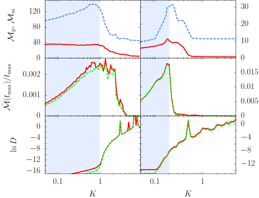
Figure 9: Top Row: ${\cal M}_{\rm p}$ (dashed/blue) and ${\cal M}_{\rm m}$ (solid/red) as a function of $K$ for the SM (left) and the HM (right) with $N=512$, $\delta K/\hbar=2.0$, and $t_{\rm max}=4000$. Middle Row: $\tilde{{\cal M}}/t_{\rm max}$ as a function of $K$ for the SM (left) and the HM (right) with $t_{\rm max}=20000$ (red/solid) and 50000 (green/dashed). Bottom Row: $D$ as a function of $K$ for the SM (left) and the HM (right) with $t_{\rm max}=20000$ (red/solid) and 50000 (green/dashed). The limit of the shaded area is $k=0.98$ (SM) and $K=0.2$ HM.

7 Conclusion

We studied numerically the non-Markovian behaviour of an environment modelled by a quantum kicked map, when it interacts – pure dephasing – with a system consisting of a qubit. In particular we centered our attention on the transition from regular to chaotic dynamics. At the extremes, i.e. either regular or chaotic the behaviour is as expected: if the environment is chaotic then we expect it to lose memory quicker and be more Markovian than an environment corresponding to regular dynamics. At the transition, where classical dynamics is mixed, unexpected behaviour manifests in the form of a peak. In the case of the standard map the peak is located almost exactly at the critical point where the last irrational torus breaks and for dynamics in the cylinder there is unbounded diffusion. For the case of the Harper map, there is no critical point. However we obtain a peak that is robust to changes in size, time and way of averaging. We conjecture that it should also correspond to a transition point in the classical dynamics. To support this conjecture we studied the fluctuations of the distance between classical trajectories (with no periodic boundaries). We found peaks at locations compatible with the results obtained for the non-Markovianity measure used.

Additionally, by studying the dependence of no-Markovianity on the initial state of the environment we first found that the main contributions to average non-Markovian behaviour come, not from regular (integrable) islands, but from the regions between chaotic and integrable which typically are complex and composed of broken tori.We were able to build classical phase space pictures from the non-Markovianity measure, where the borders between chaos and regularity are clearly highlighted. It is worth remarking that from our numerical investigations yet another feature of quantum fidelity has been unveiled: the long time fluctuations can help identify complex phase space structures like the border between chaotic and regular regions. Traditional (average) fidelity decay approaches have the aim of identifying sensitivity to perturbations, and chaos. The approach presented here, in contrast, can – from the fidelity as a function of each individual initial state – provide a clear image of the classical phase portrait and not just a global quantity from which to infer chaotic (or regular) behavior. We think that our numerics fit well within the scope of recent experimental setups [32], and some of our findings could be explored.

Finally, we should acknowledge that the validity and interpretation of the quantities used to asses how non- Markovian a quantum evolution is (including the BLP measure used here), is a subject of ongoing discussion and which remains to be decided. Even the ability of a measure of determining whether a system is Markovian is a topic of intense debate. The BLP measure tied to the system studied provided new insight particularly in the relation with the complexities of phase space. We think that the approach proposed here, i.e. a simple system coupled to a completely known environment with a feature-rich classical phase space, could provide with benchmarking possibilities for non-Markovianity measures.

Appendix A Semiclassical expression for short time decay of the fidelity amplitude

The fidelity or Loschmidt echo is the quantity originally proposed by Peres [70] to characterize sensitivity of a system to perturbation and then used to characterize quantum chaos. It is defined as

$$M(t)=|f(t)|^{2}$$ (28)

where

$$f(t)=\langle\psi_{0}|e^{iH_{\epsilon}t/\hbar}e^{-iH_{0}t/\hbar}{|\psi_{0}\rangle}$$ (29)

where $H_{\epsilon}$ is differs from $H_{0}$ by a perturbation term, usually taken as an additive $\epsilon V$ term, with $\epsilon$ a small number.

Using the initial value representation for the Van Vleck semiclassical propagator and a concept known as dephasing representation (DR), justified by the shadowing theorem, recently the following simplified semiclassical expression for the fidelity amplitude to [71, 72, 73] was obtained

$$f_{{}_{\rm DR}}(t)=\int dqdpW_{\psi}(q,p)\exp(-i\Delta S_{\epsilon}(q,p,t)/\hbar).$$ (30)

In Eq. (30) $W_{\psi}(q,p)$ is the Wigner function of the initial state $\psi$ and

$$\Delta S_{\epsilon}(q,p,t)=-\epsilon\int_{0}^{t}d\tau V(q(\tau),p(\tau))$$ (31)

is the action difference evaluated along the unperturbed classical trajectory.

For sufficiently chaotic system we can approximate the dynamics as random-uncorrelated and express the average fidelity amplitude as [64]

$$\langle f_{{}_{\rm DR}}(t)\rangle=\left[\frac{1}{N}\sum_{j}\exp(-i\Delta S_{\epsilon,j}/\hbar)\right]$$ (32)

the average is done over a complete set labeled $j$ ($N$ is the dimension of the Hilbert space) and $\Delta S_{\epsilon,j}$ is the action difference for the state $j$ at time $t=1$ (we focus on discrete time (maps), so for us it means after one step). For large enough $N$ we can approximate by a continuous expression

$$\langle f_{{}_{\rm DR}}(t)\rangle\approx\left(\int dqdp\exp[-i\Delta S_{\epsilon}(q,p)/\hbar]\right)^{t}$$ (33)

The short time decay of the AFA can be approximated by

$$|\langle f(t)\rangle|\approx e^{-\Gamma t}$$ (34)

with

$$\Gamma\approx-\ln\left|\int dqdp\exp[-i\Delta S_{\epsilon}(q,p)/\hbar]\right|$$ (35)

This expression if exact for $t=1$ and is valid for larger times the more chaotic is the system (see [64]). For both maps in Eqs. (17) and (19) we have $V=K\cos[2\pi q]$ so

$$\Gamma\approx-\ln\left|\int dqe^{-(\delta K/\hbar)\cos[2\pi q_{i}]}\right|=-\ln[|J_{0}(\delta K/\hbar)|],$$ (36)

where $J_{0}$ is the Bessel function of the first kind (with $n=0$), which is an oscillating function. When $J_{0}=0$, $\Gamma$ diverges. This means that near these values for short times fidelity decays almost to zero. Nevertheless – also depending on how chaotic the system is – after this strong decay, typically there is a large revival [74, 64].

References

References

- [1] Joos E, Zeh H D, Kiefer C, Giulini D, Kupsch J and Stamatescu I O 1996 Decoherence and the appearance of a classical world in quantum theory (Springer, Berlin)
- [2] Zurek W H 2003 Rev. Mod. Phys. 75 715–775
- [3] Breuer H P and Petruccione F 2007 The Theory of Open Quantum Systems (Oxford University Press, Oxford)
- [4] Lindblad G 1976 Comm. Math. Phys. 48 119
- [5] Gorini V, Kossakowski A and Sudarshan E C G 1976 J. Math. Phys. 17 821
- [6] Daffer S, Wódkiewicz K, Cresser J D and McIver J K 2004 Phys. Rev. A 70 010304
- [7] Breuer H P, Laine E M and Piilo J 2009 Phys. Rev. Lett. 103 210401
- [8] Rivas A, Huelga S F and Plenio M B 2010 Phys. Rev. Lett. 105 050403
- [9] Žnidarič M, Pineda C and García-Mata I 2011 Phys. Rev. Lett. 107 080404
- [10] Dente A D, Zangara P R and Pastawski H M 2011 Phys. Rev. A 84 042104
- [11] Haikka P, Goold J, McEndoo S, Plastina F and Maniscalco S 2012 Phys. Rev. A 85 060101 (R)
- [12] Clos G and Breuer H P 2012 Phys. Rev. A 86 012115
- [13] Alipour S, Mani A and Rezakhani A 2012 Phys. Rev. A 85 052108
- [14] Fiori E R and Pastawski H 2006 Chem. Phys. Lett. 420 35
- [15] Zhang P, You B and Cen L X arxiv:1302.6366
- [16] Bylicka B, Chruściński D and Maniscalco S arxiv:1301.2585
- [17] Barreiro J T, Müller M, Schindler P, Nigg D, Monz T, Chwalla M, Hennrich M, Roos C F, Zoller P and Blatt R 2011 Nature 470 486
- [18] Diehl S, Micheli A, Kantian A, Kraus B, Büchler H P and Zoller P 2008 Nature Physics 4 878
- [19] Krauter H, Muschik C A, Jensen K, Wasilewski W, Petersen J M, Cirac J I and Polzik E S 2011 Phys. Rev. Lett. 107(8) 080503
- [20] Huelga S, Rivas Á and Plenio M 2012 Physical Review Letters 108 160402
- [21] Chin A W, Huelga S F and Plenio M B 2012 Phys. Rev. Lett. 109(23) 233601 URL http://link.aps.org/doi/10.1103/PhysRevLett.109.233601
- [22] Verstraete F, Wolf M M and Cirac J I 2009 Nature Physics 5 633
- [23] Ishizaki A and Fleming G R 2009 PNAS 106 17255–17260
- [24] Liu B H, Li L, Huang Y F, Li C F, Guo G C, Laine E M, Breuer H P and Piilo J 2011 Nat. Phys. 7 931
- [25] Chiuri A, Greganti C, Mazzola L, Paternostro M and Mataloni P 2012 Scientific Reports 2 968
- [26] Liu B H, Cao D Y, Huang Y F, Li C F, Guo G C, Laine E M, Breuer H P and Piilo J 2013 Scientific Reports 3 1781
- [27] García-Mata I, Pineda C and Wisniacki D A 2012 Phys. Rev. A 86 022114
- [28] de Almeida A 1990 Hamiltonian Systems: Chaos and Quantization Cambridge Monographs on Mathematical Physics (Cambridge University Press) ISBN 9780521386708 URL http://books.google.com.mx/books?id=nNeNSEJUEHUC
- [29] Karkuszewski Z P, Jarzynski C and Zurek W H 2002 Phys. Rev. Lett. 89 170405
- [30] Quan H, Song Z, Liu X, Zanardi P and Sun C 2006 Phys. Rev. Lett. 96 140604
- [31] Lemos G B and Toscano F 2011 Physical Review E 84 016220
- [32] Lemos G B, Gomes R M, Walborn S P, Ribeiro P H S and Toscano F 2012 Nature Communications 3 1211
- [33] Poulin D, Blume-Kohout R, Laflamme R and Ollivier H 2004 Phys. Rev. Lett. 92 177906
- [34] Petitjean C and Ph Jacquod 2005 Phys. Rev. E 71 036223
- [35] Weinstein Y and Hellberg C 2005 Physical Review E 71 016209
- [36] Weinstein Y, Lloyd S and Tsallis C 2002 Phys. Rev. Lett. 89 214101
- [37] Gorin T, Prosen T, Seligman T and Žnidarič M 2006 Phys. Rep. 435 33
- [38] Ph Jacquod and Petitjean C 2009 Adv. Phys. 58 67
- [39] Goussev A, Jalabert R, Pastawski H M and Wisniacki D A 2012 Scholarpedia 7 11687
- [40] Breuer H P 2012 J. Phys. B 45 154001
- [41] Vacchini B, Smirne A, Laine E M, Piilo J and Breuer H P 2011 New J. Phys. 13 093004 ISSN 1367-2630
- [42] Heinosaari T and Ziman M 2008 Acta Physica Slovaca 58 487
- [43] Hayashi M 2006 Quantum Information (Springer, Berlin)
- [44] Lu X M, Wang X and Sun C P 2010 Phys. Rev. A 82 042103
- [45] Wolf M M, Eisert J, Cubitt T S and Cirac J I 2008 Phys. Rev. Lett. 101 150402
- [46] Zeng H S, Tang N, Zheng Y P and Wang G Y 2011 Phys. Rev. A 84 032118
- [47] Vandersypen L M K and Chuang I L 2005 Rev. Mod. Phys. 76 1037
- [48] Britton J, Sawyer B, Keith A, Wang C C, Freericks J, Uys H, Biercuk M and Bollinger J 2012 Nature 484 489
- [49] Jalabert R A and Pastawski H M 2001 Phys. Rev. Lett. 86 2490
- [50] Wißmann S, Karlsson A, Laine E M, Piilo J and Breuer H P 2012 Phys. Rev. A 86 062108
- [51] Gardiner S A, Cirac J I and Zoller P 1997 Phys. Rev. Lett. 79 4790–4793
- [52] Schack R 1998 Phys. Rev. A 57(3) 1634–1635
- [53] Georgeot B and Shepelyansky D L 2001 Phys. Rev. Lett. 86 5393–5396
- [54] Weinstein Y, Lloyd S, Emerson J and Cory D 2002 Phys. Rev. Lett. 89
- [55] Lévi B, Georgeot B and Shepelyansky D L 2003 Phys. Rev. E 67
- [56] Lévi B and Georgeot B 2004 Phys. Rev. E 70 056218
- [57] Chaudhury S, Smith A, Anderson B E, Ghose S and Jessen P S 2009 Nature 461 768
- [58] Chirikov B and Shepelyansky D L 2008 Scholarpedia 3 3350
- [59] Lichtenberg, A and Lieberman M 1992 Regular and Chaotic Dynamics, 2nd Ed. (Springer, New York)
- [60] Greene J M 1979 J. Math. Phys. 20 1183
- [61] Dana I 1995 Phys. Lett. A 197 413
- [62] Artuso R 2011 Scholarpedia 6 10462
- [63] Leboeuf P, Kurchan J, Feingold M and Arovas D 1990 Physical Review Letters 65 3076
- [64] García-Mata I, Vallejos R O and Wisniacki D A 2011 New J. Phys. 13 103040
- [65] Pineda C, Schäfer R, Prosen T and Seligman T 2006 Phys. Rev. E 73 066120
- [66] Arguelles A and Dittrich T 2005 Physica A 356 72
- [67] Ding M, Bountis T and Ott E 1990 Physics Letters A 151 395
- [68] Karney C F 1983 Physica D: Nonlinear Phenomena 8 360–380
- [69] Leboeuf P 1998 Physica D: Nonlinear Phenomena 116 8
- [70] Peres A 1984 Phys. Rev. A 30 1610
- [71] Vaníček J and Heller E J 2003 Phys. Rev. E 68 056208
- [72] Vaníček J 2004 Phys. Rev. E 70 055201
- [73] Vaníček J 2006 Phys. Rev. E 73 046204
- [74] García-Mata I and Wisniacki D A 2011 J. Phys. A: Math. Theor. 44 315101