Excision scheme for black holes in constrained evolution formulations: Spherically symmetric case

Abstract

Excision techniques are used in order to deal with black holes in numerical simulations of Einstein’s equations and consist in removing a topological sphere containing the physical singularity from the numerical domain, applying instead appropriate boundary conditions at the excised surface. In this work we present recent developments of this technique in the case of constrained formulations of Einstein’s equations and for spherically symmetric spacetimes. We present a new set of boundary conditions to apply to the elliptic system in the fully constrained formalism of Bonazzola et al. [Phys. Rev. D 70, 104007 (2004)], at an arbitrary coordinate sphere inside the apparent horizon. Analytical properties of this system of boundary conditions are studied and, under some assumptions, an exponential convergence toward the stationary solution is exhibited for the vacuum spacetime. This is verified in numerical examples, together with the applicability in the case of the accretion of a scalar field onto a Schwarzschild black hole. We also present the successful use of the excision technique in the collapse of a neutron star to a black hole, when excision is switched on during the simulation, after the formation of the apparent horizon. This allows the accretion of matter remaining outside the excision surface and for the stable long-term evolution of the newly formed black hole.

I Introduction

Relativistic simulations of astrophysical phenomena involving one or several black holes (BHs) have undergone significant improvements in the last decade, in particular with the first successful studies of binary BH systems pretorius-05 ; campanelli-06 ; baker-06 . One of the major difficulties in performing such simulations is the handling of the physical singularity of the BH, where some physical fields may diverge. In order to cope with this problem, essentially two types of methods have been proposed in the literature: i) excision, where the singularity, together with its neighborhood, is removed from the computational domain and eventually replaced by boundary conditions (see e.g. Refs. seidel-92 ; lehner-00 ); and ii) punctures, where the BH is set in such initial data that the physical singularity is not included, but instead the spatial hypersurface containing the initial data follows a wormhole through to another copy of spacetime, which is compactified and its infinity is reduced to a point, the “puncture” (see e.g. Refs. BraBru97 ; hannam-07 ). The wormhole topology is prescribed analytically in the conformal factor [see Eq. (2) below], which diverges at the puncture location.

Both of these approaches have been successfully applied in simulations of binary BH systems, but with different formulations of Einstein equations and gauge choices: excision has been used in conjunction with the generalized harmonic gauge pretorius-05 ; boyle-07 , and punctures have usually been associated with the so-called BSSN (from Baumgarte-Shapiro baumgarte-99 Shibata-Nakamura shibata-95 ) formulation campanelli-06 ; baker-06 . All these studies use free evolution schemes, in which the constraint equations arising in the 3+1 decomposition of Einstein equations are not enforced during the evolution. If the constraint equations are satisfied initially, they are also satisfied during the evolution theoretically, but this is not necessarily the case in numerical simulations. In these formulations, the constraint equations are satisfied by the initial data and then monitored during the evolution to check the validity of the numerical solution.

In such free evolution schemes, most of the resulting partial differential equations (PDEs), coming from Einstein and matter equations (in the case of nonvacuum spacetimes), are of hyperbolic type. In particular, when suitable gauge conditions are chosen, their characteristics, computed inside the BH (apparent) horizon, are all directed towards where the singularity is located in the spacelike hypersurface. This means that in these schemes, within the excision approach and adopting excision surfaces lying inside the apparent horizon (AH) such that their evolution world tubes are of spacelike character, there is no need for imposing any inner boundary condition (see, e.g., Ref. Dorband06 , where the excision sphere was placed sufficiently close to the horizon).

However, when solving constraints arising in the 3+1 formulation of Einstein’s equations, the elliptic nature of these PDEs requires that correct corresponding boundary conditions at the excision surface have to be defined and tested. Otherwise, incorrect boundary conditions will not give the correct physical content for the numerical solution and, therefore invalidate the whole simulation. This is particularly true in the case of a Fully Constrained Formulation (FCF), such as the one devised by Bonazzola et al. FCF , where the constraint equations are regularly solved as part of the elliptic set of equations and enforced during the numerical simulation. It has been checked that in the FCF all the characteristics of the hyperbolic sector point towards the singularity when a coordinate system adapted to the dynamical spacelike excision world tube is used in the evolution Jaramillo .

A geometric approach to defining proper boundary conditions for the elliptic part of Einstein’s equations has been undertaken on the basis of the isolated horizon paradigm CooPfe04 ; jaramillo-04 ; DaiJarKri04 ; gourgoulhon-06 ; CauCooGri06 ; Jaramillo:2009cc or the dynamical “trapping horizon” concept Jaramillo . They have been successfully applied to stationary spacetimes jaramillo-07 ; vasset-09 , which can then be used as initial data for further dynamical evolutions.

In this paper, we propose a different approach for the definition of boundary conditions in the FCF formulation using the excision technique in dynamical spacetimes, with the motivation of simulating astrophysical scenarios like a star collapsing to a BH. In this context, initial data are usually regular and no BH is present yet. During the simulation, a BH forms and, particularly when using singularity-avoiding time coordinates (e.g. maximal slicing), an AH is found before the appearance of the physical singularity shapiro-80 . When no symmetry is assumed, the AH does not have a simple shape in general and, therefore, it is not easy to use it numerically as an excision surface to impose boundary conditions. Here, we suggest using an arbitrary but nearby sphere inside the AH to define simple and appropriate boundary conditions for the elliptic system of PDEs in the FCF of Einstein’s equations, in the particular case of spherical symmetry. Numerical codes assuming spherical symmetry which include complex microphysics are nowadays still relevant; for example, spherically symmetric relativistic simulations were used to study the influence of different microphysics and equations of state in the formation of the BH in Refs. Peres13 ; Nakazato12 ; OConnor11 , instead of using simulations without any symmetry assumptions, due to the very long simulation times involved. In the case of no symmetry assumptions, we plan to follow similar ideas for using the excision technique in dynamical evolutions, but this study is beyond the scope of the present work.

We will describe how the excision technique is used in dynamical evolutions and show the practical applicability of this approach in the case of a Schwarzschild BH spacetime, the accretion of a scalar field into a spherical BH and the collapse of a neutron star to a BH. Previous works by Scheel et al. scheel-95 and Rinne and Moncrief rinne-13 have presented similar approaches in constrained formulations in spherical symmetry, too. Scheel et al. scheel-95 have considered the situation of dust collapse in the Brans-Dicke theory of gravity, whereas Rinne and Moncrief rinne-13 have studied scalar and Yang-Mills fields coupled to gravity in a constant-mean-curvature slicing. Scheel et al. scheel-95 set the excision boundary at the AH, at a fixed radial coordinate; the main difference with this work is that we here set the excision boundary to be an arbitrary sphere located strictly inside the AH, and let this AH evolve in time. This approach allows in particular for a very straightforward extension to spacetimes without symmetries, where the AH can form with a shape deviating from a coordinate sphere. The latter approach was also followed in the work of Rinne and Moncrief rinne-13 , where the value of the conformal lapse function was frozen and evolution equations were used to update the values of the remaining variables at the excision surface. Here we propose and analyze a different prescription for the boundary conditions at the excision surface, that underline the geometric features of the system.

The paper is organized as follows. The FCF of Einstein’s equations is briefly overviewed in Sec. II, which also contains some remarks in the spherically symmetric case. In Sec. III we describe the excision method, including our excision region and the boundary conditions imposed on each slice. Section IV discusses numerical results. A summary of our conclusions is given in Sec. V. We use units in which $c=G=M_{\odot}=1$. Greek indices run from 0 to 3, latin indices from 1 to 3, and we adopt the standard convention for the summation over repeated indices. $\partial_{\alpha}$ denotes partial derivatives.

II Fully Constrained Formulation

Given an asymptotically flat spacetime $({\cal M},g_{\mu\nu})$, we consider a 3+1 splitting by spacelike hypersurfaces $\Sigma_{t}$, denoting timelike unit normals to $\Sigma_{t}$ by $n^{\mu}$. The spacetime on each spacelike hypersurface $\Sigma_{t}$ is described by the pair $(\gamma_{ij},K^{ij})$, where $\gamma_{\mu\nu}=g_{\mu\nu}+n_{\mu}n_{\nu}$ is the Riemannian metric induced on $\Sigma_{t}$. We choose the convention $K_{\mu\nu}=-\frac{1}{2}{\cal L}_{\bf{n}}\gamma_{\mu\nu}$ for the extrinsic curvature. With the lapse function $N$ and the shift vector $\beta^{i}$, the Lorentzian metric $g_{\mu\nu}$ in the 3+1 formalism can be expressed in coordinates $(x^{\mu})$ as

$$g_{\mu\nu}dx^{\mu}dx^{\nu}=-N^{2}dt^{2}+\gamma_{ij}(dx^{i}+\beta^{i}dt)(dx^{j}+\beta^{j}dt).$$ (1)

As in Ref. FCF , we introduce a time-independent flat metric $f_{ij}$, which satisfies ${\cal L}_{\bf{t}}f_{ij}=\partial_{t}f_{ij}=0$ and coincides with $\gamma_{ij}$ at spatial infinity. With the definitions $\gamma:=\det\gamma_{ij}$ and $f:=\det f_{ij}$, we introduce the following conformal decomposition of the spatial metric,

$$\gamma_{ij}=\psi^{4}\tilde{\gamma}_{ij},\;\;\;\psi=(\gamma/f)^{1/12}.$$ (2)

The difference between the conformal metric and the flat fiducial one is denoted by $h^{ij}$, $h^{ij}:=\tilde{\gamma}^{ij}-f^{ij}$. The chosen prescriptions for the gauge variables in Ref. FCF are the maximal slicing,

$$K=0,$$ (3)

and the so-called generalized Dirac gauge,

$${\cal D}_{i}\tilde{\gamma}^{ij}={\cal D}_{i}h^{ij}=0,$$ (4)

where $K=\gamma^{ij}K_{ij}$ denotes the trace of the extrinsic curvature and ${\cal D}_{k}$ stands for the Levi-Civita connection associated with the flat metric $f_{ij}$. Finally, we introduce the conformal decomposition

$$\hat{A}^{ij}:=\psi^{10}K^{ij}.$$ (5)

In this formulation, Einstein’s equations result in a coupled elliptic-hyperbolic system: the elliptic sector acts on the variables $\psi$, $N$ and $\beta^{i}$, while the hyperbolic sector acts on $h^{ij}$ and $\hat{A}^{ij}$. More details of the analysis of both sectors can be found in Refs. CC08 ; CC09 .

The decomposition of $\hat{A}^{ij}$ in longitudinal and transverse-traceless (TT) parts

$$\hat{A}^{ij}=(LX)^{ij}+\hat{A}^{ij}_{\mathrm{TT}},$$ (6)

where $(LX)^{ij}:={\cal D}^{i}X^{j}+{\cal D}^{j}X^{i}-\frac{2}{3}f^{ij}{\cal D}_{k}X^{k}$ and ${\cal D}_{i}\hat{A}^{ij}_{\mathrm{TT}}=0$, can be considered motivated by the local uniqueness properties of the elliptic sector shown in Ref. CC09 .

We decompose classically the energy-momentum tensor, $T^{\mu\nu}$, measured by the observer of 4-velocity $n^{\mu}$ (Eulerian observer), in terms of the energy density $E:=T_{\mu\nu}n^{\mu}n^{\nu}$, the momentum density $S_{i}:=-\gamma^{\mu}_{i}T_{\mu\nu}n^{\nu}$, and the stress tensor $S_{ij}:=T_{\mu\nu}\gamma^{\mu}_{i}\gamma^{\nu}_{j}$, with $S:=\gamma^{ij}S_{ij}$ being its trace.

The resulting elliptic equations in the FCF are

$$\tilde{\Delta}\psi = -2\pi\psi^{-1}E^{*}-\frac{\tilde{\gamma}_{il}\tilde{\gamma}_{jm}\hat{A}^{lm}\hat{A}^{ij}}{8\psi^{7}}+\frac{\psi\tilde{R}}{8},\hskip 19.91684pt$$ (7)

$$\tilde{\Delta}(N\psi) = \left[2\pi\psi^{-2}(E^{*}+2S^{*})\right.$$ (8)

$$\left.+\left(\frac{7\tilde{\gamma}_{il}\tilde{\gamma}_{jm}\hat{A}^{lm}\hat{A}^{ij}}{8\psi^{8}}+\frac{\tilde{R}}{8}\right)\right](N\psi),$$

$$\tilde{\Delta}\beta^{i} = 16\pi N\psi^{-6}\tilde{\gamma}^{ij}(S^{*})_{j}+\hat{A}^{ij}{\cal D}_{j}(2N\psi^{-6})$$ (9)

$$-2N\psi^{-6}\Delta^{i}_{kl}\hat{A}^{kl},$$

where the operator $\tilde{\Delta}$ is defined as

$$\tilde{\Delta}\psi=\tilde{\gamma}^{kl}{\cal D}_{k}{\cal D}_{l}\psi$$ (10)

(analogously for $N\psi$) and

$$\tilde{\Delta}\beta^{i}=\tilde{\gamma}^{kl}{\cal D}_{k}{\cal D}_{l}\beta^{i}+\frac{1}{3}\tilde{\gamma}^{ik}{\cal D}_{k}{\cal D}_{l}\beta^{l},$$ (11)

$E^{*}:=\psi^{6}E$, $S^{*}:=\psi^{6}S$, $(S^{*})_{i}:=\psi^{6}S_{i}$,

$$\tilde{R}=\frac{1}{4}\tilde{\gamma}^{kl}{\cal D}_{k}h^{mn}{\cal D}_{l}\tilde{\gamma}_{mn}-\frac{1}{2}\tilde{\gamma}^{kl}{\cal D}_{k}h^{mn}{\cal D}_{n}\tilde{\gamma}_{ml}$$ (12)

is the scalar 3-curvature of the conformal metric $\tilde{\gamma}_{ij}$, and

$$\Delta^{i}_{jk}=\frac{1}{2}\tilde{\gamma}^{kl}({\cal D}_{i}\tilde{\gamma}_{lj}+{\cal D}_{j}\tilde{\gamma}_{il}-{\cal D}_{l}\tilde{\gamma}_{ij})$$ (13)

is the difference between Christoffel symbols of the conformal and flat metrics.

The resulting hyperbolic equations are evolution equations for $h^{ij}$ and $\hat{A}^{ij}$,

$$\partial_{t}h^{ij} = 2N\psi^{-6}\hat{A}^{ij}+\beta^{k}{\cal D}_{k}h^{ij}$$ (14)

$$-\tilde{\gamma}^{ik}{\cal D}_{k}\beta^{j}-\tilde{\gamma}^{kj}{\cal D}_{k}\beta^{i}+\frac{2}{3}\tilde{\gamma}^{ij}{\cal D}_{k}\beta^{k},$$

$$\partial_{t}\hat{A}^{ij} = (S_{\hat{A}})^{ij},$$ (15)

where the explicit expression for the source $(S_{\hat{A}})^{ij}$ can be found in Ref. CC12 .

If a TT decomposition is performed for $\hat{A}^{ij}$, an extra elliptic equation for the vector $X^{i}$ is added and Eq. (15) can be viewed as an evolution equation for $\hat{A}^{ij}_{\mathrm{TT}}$.

II.1 Spherical symmetry

It has been proven in Ref. CC11 that a spherically symmetric spacetime can be locally foliated by a maximal slicing and by using isotropic coordinates for the spatial metric onto the spatial hypersurfaces $\Sigma_{t}$. This statement refers to neighborhoods, and does not involve global prescriptions or boundaries. The FCF in spherical symmetry and with topologically $\mathbb{R}^{3}$ spatial hypersurfaces $\Sigma_{t}$ reduces to the isotropic gauge, where $\tilde{\gamma}^{ij}=f^{ij}$. This is not true anymore for more general topologies, like the $\mathbb{R}^{3}-{\cal B}$ case, where ${\cal B}$ is a ball, when general boundary conditions on the boundary of ${\cal B}$ are given. In a nonconvex topology such as $\mathbb{R}^{3}-{\cal B}$, the expression for $\tilde{\gamma}^{ij}$ evolving in time in the FCF in spherical symmetry is instead given by

$$\tilde{\gamma}^{ij}(t)=\left(\begin{tabular}[]{ccc}$\left(1+\frac{\omega(t)}{r^{3}}\right)^{\frac{2}{3}}$&0&0\\ 0&$\left(1+\frac{\omega(t)}{r^{3}}\right)^{-\frac{1}{3}}$&0\\ 0&0&$\left(1+\frac{\omega(t)}{r^{3}}\right)^{-\frac{1}{3}}$\end{tabular}\right),$$ (16)

where $\omega(t)$ is a real and twice-derivable function of time $t$. A proof of this statement is presented in Appendix A. Note that on $\mathbb{R}^{3}$, $\omega=0$ is required at the origin for metric regularity. If a ball containing the origin is excised and the value for $\omega$ is not zero at the excision boundary, the spatial metric is not necessarily expressed as a conformally flat one.

Since the value for $\omega$ can be chosen arbitrarily taking into account the previous general expression for $\tilde{\gamma}^{ij}$ (it represents just a gauge freedom, as the Dirac gauge is a differential one), the spatial metric can be expressed as a conformally flat one, i.e., $\tilde{\gamma}^{ij}=f^{ij}$, or equivalently, $h^{ij}=0$. Note that in this case Eq. (14) is a time-independent prescription for $\hat{A}^{ij}$,

$$\hat{A}^{ij}=\frac{\psi^{6}}{2N}\left(\tilde{\gamma}^{ik}{\cal D}_{k}\beta^{j}+\tilde{\gamma}^{kj}{\cal D}_{k}\beta^{i}-\frac{2}{3}\tilde{\gamma}^{ij}{\cal D}_{k}\beta^{k}\right),$$ (17)

Equations (7–9) can be solved to obtain $N$, $\psi$ and $\beta^{i}$, and Eq. (15) is a redundant condition in the bulk. This redundant condition will be used as a compatibility condition for the prescription of boundary conditions in the constrained system resolution.

In a general spacetime with no spherical symmetry $h^{ij}=0$ cannot be imposed, and $h^{ij}$ and $\hat{A}^{ij}$ have to be evolved in time. Boundary conditions on the excision boundary for hyperbolic equations may or may not be imposed, depending on the characteristic structure of the system. This is not the case for elliptic equations, for which incorrect boundary conditions invalidate the solution in the whole domain. The general case (no spherically symmetric spacetimes) is beyond the scope of this work and will be analyzed in future studies.

III Excision method

Due to the singular character of BH interior solutions, measures have to be taken in numerical simulations of BH spacetimes. Quite a number of codes relying on hyperbolic formulations of Einstein’s equations are based on an adaptive slicing which is typically designed to avoid the BH singularity by coordinate stretching and using a proper shift vector. This is the case of the BSSN formulation in combination with the puncture method, which is very popular in binary BH simulations. An alternative approach is known as stuffed BHs, where one fills BH interiors with unimportant (but regular) junk data in a hyperbolic formulation, and then evolves the regularized spacetime arbona-98 ; brown-07 .

In this work, we want to present how the excision technique can be used in the FCF in spherically symmetric spacetimes, where the presence of elliptic PDEs has to be taken into account. This technique consists in removing from each spatial hypersurface $\Sigma_{t}$ the open interior of a topological sphere ${\cal S}^{2}$, and solving Einstein’s equations in the remaining hypersurface. The sphere is assigned both physical and geometrical characteristics, tailored so that it is located strictly inside the AH of the modeled BH region, and so that it encloses the gravitational singularity. Those properties are then encoded as boundary conditions of the available elliptic equations to be solved for.

In BH initial data problems, a natural approach consists in placing the excision sphere at the outermost marginally outer trapped surface in the initial slice, namely the AH. Much work has been done in this field, including how to impose this prescription and transcribe it in terms of 3+1 spacetime metric quantities (see, e.g., Refs. CooPfe04 ; jaramillo-04 ; DaiJarKri04 ; gourgoulhon-06 ; CauCooGri06 ; Jaramillo:2009cc ). In the evolution case, the set of excision spheres at every $\Sigma_{t}$ can be prescribed to describe a hypertube of marginally outer trapped surfaces, leading to a trapping horizon as outlined in Ref. Jaramillo . Here we will rather follow a more generic approach in which the excision surface is not enforced at the BH AH, but rather at the interior of the AH world tube.

III.1 Excision surface geometry

We first define the geometrical setting of the excision surface. Notice that these definitions do not depend on the matter content of the spacetime, being valid for vacuum and nonvacuum spacetimes. Let ${\cal S}_{t}$ be a topological 2-sphere embedded in $\Sigma_{t}$, and its induced 2-metric is $q_{ab}$. Let $s^{\mu}$ be the unit outward-directed spacelike vector normal to ${\cal S}_{t}$, that is also tangent to $\Sigma_{t}$. Let $\mathcal{H}$ be the hypertube formed by the set of excision spheres at every $\Sigma_{t}$. At the excision surface, three other vector fields are defined: the outward and inward future-directed null vectors

$$l^{\mu}=(n^{\mu}+s^{\mu})/\sqrt{2},\;\;k^{\mu}=(n^{\mu}-s^{\mu})/\sqrt{2},$$ (18)

respectively, and the evolution vector on $\cal H$ normal to sections ${\cal S}_{t}$ and carrying ${\cal S}_{t}$ onto ${\cal S}_{t+\delta t}$

$$h^{\mu}=Nn^{\mu}+bs^{\mu},$$ (19)

which we adapt to the 3+1 evolution vector $t^{\mu}=Nn^{\mu}+\beta^{\mu}$, so that $b=\beta^{i}s_{i}$ (note that $b$ is only defined at $\cal H$). This means that the excision surface is kept at the same spatial coordinate location along the evolution. Two additional geometric quantities are the scalar outward expansion $\theta^{(l)}$ and outward shear $\sigma_{ab}$ along $l^{\mu}$, defined as

$${\cal L}_{l}\epsilon^{\cal S}_{ab} = \theta^{(l)}\epsilon^{\cal S}_{ab},$$ (20)

$$\sigma^{(l)}_{ab} = \frac{1}{2}\left[{\cal L}_{l}q_{ab}-\theta^{(l)}q_{ab}\right],$$ (21)

where $\epsilon^{\cal S}_{ab}$ is the area element on ${\cal S}_{t}$. Analogously, the inward expansion $\theta^{(k)}$ and the corresponding shear can be defined.

For a Schwarzschild BH, in the case of adapting the excision surface to the AH, the excision world tube $\cal H$ is a null hypersurface, meaning that the time evolution vector $h^{\mu}$ at the excision surface is null. This provides the following relationship between metric quantities at the AH: $b=N$. The outward expansion $\theta^{(l)}$ can be expressed as follows [see e.g. Eq. (11.8) in Ref. gourgoulhon-06 ]:

$$\psi^{2}\,\theta^{(l)}=4\tilde{s}^{i}\tilde{D}_{i}\ln\psi+\tilde{D}_{i}\tilde{s}^{i}+K_{ij}\frac{\tilde{s}^{i}\tilde{s}^{j}}{\psi^{2}},$$ (22)

where $\tilde{s}^{i}:=\psi^{2}s^{i}$ and $\tilde{D}$ is the Levi-Civita connection associated with the conformal metric $\tilde{\gamma}_{ij}$. This relation could be used as a (nonlinear) Robin boundary condition on the conformal factor in order to compute initial data. In particular, the outward expansion $\theta^{(l)}$ vanishes if the excision surface is placed at the AH, or can be prescribed to be negative to place the excision surface inside the AH, as we shall do here. One can set $h^{ij}=0$ at the boundary and on the whole spacetime, due to the particular form that the Dirac gauge takes in spherical symmetry (see Appendix A).

The value of the lapse subsists at the excision boundary as a free condition for initial data: since the maximal slicing gauge provides us only with an elliptic constraint on the bulk, one can still choose freely the value at the inner excision surface. In the case of a dynamical evolution of a spherically symmetric BH, the value of the lapse at the excision surface has to be consistent with the assumption $h^{ij}=0$, as it is described in the next subsection.

III.2 Dynamical approach in the spherically symmetric case

We consider now the time-dependent case in spherical symmetry involving matter content. Such situations include pure gauge evolutions (as illustrated in Sec. IV.2) and matter evolution (as illustrated here for the particular case of a scalar field, see Sec. IV.3, and for the collapse of a neutron star to a BH, see Sec. IV.4). As an astrophysical application, we have in mind the BH formation in stellar gravitational collapse simulations. Starting from a simulation for regular data evolving in $\mathbb{R}^{3}\times[0,t_{0}]$, a trapped region forms at a given time $t=t_{0}$. To pursue the simulation long enough to study the subsequent evolution of the BH, one performs excision inside the trapped region, switching to a simulation in $(\mathbb{R}^{3}-{\cal B})\times[t_{0},+\infty)$. The algorithm has the three following conditions to fulfill: i) for numerical stability reasons, a transition between the two topologies has to occur smoothly, meaning that all the metric quantities solved for must be continuous and derivable in time at $t=t_{0}$; ii) dynamical excision has to avoid coordinate stretching and high gradient fields that would cause high and increasing inaccuracies in the computation; iii) the Schwarzschild solution should be recovered in the stationary limit.

The outermost trapped surface corresponding to the adopted spherically symmetric slicing can be located with an AH finder. Since there is no previous control on the geometry of this trapped region, the outermost trapped surface might be stretched or deformed in three-dimensional models, and thus is not in general an optimal candidate for the excision surface, unless we make an adaptation of the coordinates to the horizon that would imply a remapping of all data on the slice and likely introduce complexity in the problem and a copious amount of noise. A recent approach following this idea can be found in Ref. Hemberger for the simulation of binary BH spacetimes.

At time $t=t_{0}$, we choose the excision surface ${\cal S}_{t_{0}}$ to be located strictly inside the trapped region. The quantities $N$, $\psi$ and $\beta^{i}$ are determined at ${\cal S}_{t_{0}}$ by the previous evolution and are employed as initial values for the subsequent evolution. The outgoing scalar expansion is generically (and on average) negative, $\theta^{(l)}_{t=t_{0}}\leq 0$.

Once the initial excised surface has been chosen, one needs to determine a geometrical prescription for the evolution of the excision surface in time, i.e. to characterize the excision hypertube. If the initial surface were the AH, one could prescribe it to span an AH world tube in time, by imposing the vanishing of the outward expansion $\theta^{(l)}$ at all times on the sphere of constant radius $R$ Jaramillo . Contrary to the stationary case, we do not have in general $b=N$ at the horizon. In particular, in the spherically symmetric case one has [see e.g. Eq. (38) in Ref. Jaram11 , with $2C=b^{2}-N^{2}$ and vanishing angular derivatives]

$$\frac{b^{2}-N^{2}}{2}=-\frac{{\sigma^{(l)}_{\mu\nu}}{\sigma^{(l){\mu\nu}}}+T_{\mu\nu}l^{\mu}l^{\nu}}{{\cal L}_{k}\theta^{(l)}}\ .$$ (23)

Under the null energy condition the numerator is nonpositive, so that the fulfillment of an outer trapping horizon condition Hayward:1993wb , namely ${\cal L}_{k}\theta^{(l)}<0$, implies $b\geq N$. In this case the horizon is either null (stationary case), or spacelike (dynamical case), depending on whether the energy flux vanishes across the BH horizon. Unfortunately, spherically symmetric trapping horizons do not necessarily fulfill the (stability) outer condition Booth:2005ng , so that a priori we cannot guarantee in general that $\cal H$ is spacelike in the dynamical case. This, together with the desire to avoid a coordinate adaption of the excision surface to the AH, leads us to choose an excision sphere strictly inside the AH and look for an appropriate characterization of the excision world tube. For instance, one could also impose a (nonpositive) value of the expansion throughout the evolution, which would also determine a hypertube geometry.

Here we will rather follow an effective approach in which we control the radial component $b$ of the evolution vector $h^{\mu}$ on an excised coordinate sphere located strictly inside the AH. From $b=\beta^{i}s_{i}=\psi^{2}\beta^{i}\tilde{s}_{i}$, it follows in spherical symmetry that $b=\beta^{r}\psi^{2}$. The imposition of a constant value in time of $b$ at the excised surface, given by the data at $t=t_{0}$, provides us with a simple boundary condition for the shift vector through time. We want the excision hypertube to be spacelike, so that the quantity $(b-N)$ should remain positive. Although we do not impose this condition directly, we monitor $b-N$ along the evolution so that $b$ could be dynamically adapted if needed to guarantee the spacelike character of $\cal H$.

The values for $\psi$, $N$ and $h^{ij}$ have yet to be determined. The trace part of the evolution equations gives a consistent time evolution for $\psi$, valid everywhere and at all time [see, e.g., Eq. (42) of Ref. FCF ],

$$\partial_{t}\psi=\beta^{k}{\cal D}_{k}\psi+\frac{\psi}{6}{\cal D}_{k}\beta^{k}.$$ (24)

This equation, following from the kinematic definition of the extrinsic curvature, provides an additional coherent boundary condition for the conformal factor, which is obtained by solving the corresponding (elliptic) Eq. (7) with this boundary condition at the excised surface. The value of the lapse at the excised surface is the last (gauge) freedom left in the algorithm. We address this issue by making use of the form for $\tilde{\gamma}^{ij}$ in a $(\mathbb{R}^{3}-{\cal B})$ topology in Eq. (16). In particular, adopting the gauge $\omega(t)=0$ fixes the remaining degree of freedom in the system and, in particular, fixes the value of the lapse on the excised surface. Indeed $\tilde{\gamma}^{ij}$ adopts then a conformally flat form (or equivalently $h^{ij}=0$) at all times, and by using Eq. (15) to update the extrinsic curvature at the excised surface we can fix the boundary condition for the lapse from any nondegenerate component of Eq. (14); for instance,

$$N=\frac{\psi^{6}(L\beta)^{ij}s_{i}s_{j}}{2\hat{A}^{ij}s_{i}s_{j}}.$$ (25)

Our strategy can be summarized as follows: updated values for $\psi$ and $\hat{A}^{ij}$ at the excised surface are obtained by solving Eqs. (24) and (15), respectively; the imposition of constant $b$ and Eq. (25) are used to obtain updated values of $N$ and $\beta^{i}$ at the excised surface; finally, $h^{ij}$ is vanishing throughout the evolution. During the numerical simulation, we check that $(b-N)\geq 0$ (see Sec. IV); under the choice of an excision world tube closely tracking the AH from its interior, this quantity is indeed expected to be non-negative for matter satisfying standard energy conditions in stellar collapses [note however that in scenarios not considered here that involve much larger BHs, the denominator in Eq. (23) can actually change sign, cf. Booth:2005ng ]. With these boundary conditions, all elliptic equations can be solved in the numerical domain for all times, and no evolution equations are solved in the bulk.

In this approach for using the excision technique we have not considered the TT decomposition of the conformal extrinsic curvature given by Eq. (15), motivated by a uniqueness pathology of the elliptic sector. We find in our numerical simulations of spherically symmetric spacetimes that the given boundary conditions at the excised surface for solving the elliptic equations are enough to avoid any convergence problem in the numerical resolution of the elliptic sector. However, this question is open for more general spacetimes. In any case, the value of the $X^{i}$ vector of the TT decomposition of the conformal extrinsic curvature at the excised surface is actually a degree of freedom IsaCoconutM2009 .

III.3 Convergence to a stationary solution

Let us comment here about the convergence of metric fields to stationary values in our approach. Indeed, we find in our numerical simulations that the metric exponentially converges to a stationary solution. This fact means that the foliation induced by the boundary conditions described in Sec. III.2 is such that the coordinates adapt to the stationarity of the spacetime. Since no evolution equations for $h^{ij}$ and $\hat{A}^{ij}$ are computed in the bulk in this approach, and solutions to elliptic equations are determined by the boundary conditions at the excised surface, we should focus on the analysis of the values of the metric variables at the excised surface. The value for $b$ is fixed to be constant at the excised surface, so a convergence of the conformal factor at the excised surface to a stationary value will imply also a convergence of the shift vector at the excised surface to a stationary value. The evolution of the lapse $N$ at the excised surface should be such that it is compatible with the setting $h^{ij}=0$ in the whole spacetime. This setting should in turn be compatible with coordinates adapted to stationarity.

We therefore focus on the value of the conformal factor $\psi$ at the excised surface, whose evolution is governed by Eq. (24). Let us define $\hat{\beta}=\beta^{r}\psi^{2}$, which coincides with $b$ at the excised surface. Equation (24) can be rewritten in terms of $\psi$ and $\hat{\beta}$ as

$$\partial_{t}\psi=\frac{\partial_{r}\hat{\beta}}{6\psi}+\frac{2\hat{\beta}}{3}\frac{\partial_{r}\psi}{\psi^{2}}+\frac{\hat{\beta}}{3r\psi}.$$ (26)

Here we keep $b$ constant at its initial given value at the excised surface, located at a fixed coordinate radius, say $R>0$, during the evolution: $b_{|R}=\hat{\beta}_{|R}=b_{0}>0$ [since in the initial data $N$ is strictly positive and $(b-N)$ is positive, $b_{0}$ is strictly positive, too].

Motivated by the results we observe in our numerical simulations, let us assume in the present consistency analysis that $(\partial_{r}\hat{\beta})_{|R}$ is negative and does not change significantly during the evolution, so $(\partial_{r}\hat{\beta})_{|R}\approx b_{1}<0$, with $b_{1}$ being a constant. These assumptions are compatible with the ones found in our numerical simulations with an excised surface strictly inside the AH. In particular, such hypotheses (constant and negative value for $b_{1}$) are checked in the different numerical simulations of Sec. IV.

Let us assume a profile for $\psi$ of the form

$$\psi\approx 1+\frac{c(t)}{r^{p}},\;\;p\geq 1.$$ (27)

This profile can be considered as the one containing the leading term for $r$, taking into account that $\psi\to 1$ when $r\to\infty$ (first term) and that the conformal factor should diverge at the center of the BH ($p\geq 1$). Therefore, $\partial_{r}\psi\approx-p\;c(t)/r^{p+1}$ and $\partial_{t}\psi\approx c^{\prime}(t)/r^{p}$, where the prime denotes the derivative.

The hypotheses assumed here are not imposed during the numerical evolution of the system; they are used only to analyze the behavior of the metric variables in stationary spacetimes.

Taking into account previous assumptions, Eq. (26) at the excised radius $R$ is rewritten as

$$c^{\prime}(t)=\frac{c_{1}}{[R^{p}+c(t)]}+\frac{c_{2}}{[R^{p}+c(t)]^{2}},$$ (28)

where

$$c_{1} = \frac{R^{2p-1}}{3}\left(\frac{b_{1}\,R}{2}-b_{0}(2p-1)\right)<0,$$ (29)

$$c_{2} = \frac{2b_{0}\,p\,R^{3p-1}}{3}>0,$$ (30)

are constants. We can integrate the previous differential equation, expressed in an implicit way,

$$t=f(R^{p}+c(t)) = c_{0}+\frac{[R^{p}+c(t)]^{2}}{2c_{1}}-\frac{c_{2}[R^{p}+c(t)]}{c_{1}^{2}}$$ (31)

$$+\frac{c_{2}^{2}}{c_{1}^{3}}\log|c_{1}[R^{p}+c(t)]+c_{2}|,$$

where $c_{0}$ is an integration constant. The implicit equation for $[R^{p}+c(t)]$ is well defined in both branches $c_{1}[R^{p}+c(t)]+c_{2}<0$ and $c_{1}[R^{p}+c(t)]+c_{2}>0$. The function $f$ has a monotonic behavior on each branch (increasing or decreasing depending on the specific one). In both branches, the range of $t$ is $\mathbb{R}$. For the initial value $[R^{p}+c(t=t_{0})]=-c_{2}/c_{1}$, the solution of Eq. (28) is simply the constant value $[R^{p}+c(t)]=-c_{2}/c_{1}$. For initial values that are close by, an exponential convergence of $[R^{p}+c(t)]$ to the value $-c_{2}/c_{1}$ is found when $t\to+\infty$.

This discussion shows, under the assumed conditions, that we shall obtain exponential convergence to stationary values for the conformal factor $\psi$, and therefore to all metric variables, if the initial data are close enough to the stationary solution. This fact is checked numerically in Sec. IV.

IV Numerical Results

The excision technique has been used in several numerical codes with different coordinates and slicings (e.g., in Ref. Marsa96 a null-based slicing using minimally modified ingoing Eddington-Finkelstein coordinates was used to evolve a BH using the excision technique almost 20 years ago). In order to illustrate that the excision method presented in Sec. III for the FCF, in which maximal slicing and Dirac generalized gauge are chosen, works well in practice in a numerical code, we have implemented and tested it in two toy models, detailed in the following subsections: the setup is presented in Sec. IV.1, and it is applied to the evolution of a Schwarzschild BH in Sec. IV.2, and to the accretion of a massless scalar field in Sec. IV.3. We have also implemented the excision technique in a full simulation of the collapse of a neutron star to a BH in spherical symmetry in Sec. IV.4.

IV.1 Setup

We consider spherically symmetric spacetimes in the three following physical scenarios: the evolution of a slicing of a Schwarzschild BH (vacuum spacetime) in Sec. IV.2, the spherical accretion of a massless scalar field onto an existing BH in Sec. IV.3 and the collapse of an unstable neutron star to a BH. In all cases, we use spherical (polar) coordinates and in the first two scenarios, we start from an existing BH, with the excision sphere located at the coordinate radius $r=1$. As stated in Sec. II.1, the hypothesis of a spherically symmetric spacetime in which adapted boundary conditions are chosen, such that $\omega(t)=0$ implies that, as far as the gravitational field is concerned, we only need to solve for $N$, $\beta^{i}$ and $\psi$.

In the first two scenarios we start from initial data which already contain a BH and then evolve the system in the above-described excision scheme. Therefore we need to construct initial data at $t=t_{0}=0$ by solving the elliptic system (7)-(9), with the stress-energy tensor being either zero (vacuum) in the Schwarzschild BH evolution, or given by expressions (42)-(44) of Appendix B in the case of the scalar field accretion. The initial excision surface is chosen as a sphere with a given (arbitrary) value of the outward expansion [Eq. (20)] $\theta^{(l)}(t=0,r=1)=\theta^{(l)}_{0}$, prescribed to be negative. This guarantees that the initial excision surface is inside the AH, which then is located using an AH finder. Initial data boundary conditions are needed for the elliptic system and are taken as follows:

• Setting $\theta^{(l)}_{0}$ and using Eq. (22), a (nonlinear) Robin boundary condition is obtained for the conformal factor $\psi$.

• The boundary value of the lapse $N$ is fixed yielding a Dirichlet condition.

• A value is prescribed for the quantity $b-N$ [see Eq. (19)], from which one can get a Dirichlet boundary condition for the radial component of the shift $\beta^{r}$, the other two components ($\beta^{\theta},\beta^{\varphi}$) being zero in spherical symmetry.

The elliptic system giving the metric functions is solved iteratively, starting from a first guess (flat metric) and inverting linear Laplace operators with the library lorene lorene , using multidomain spectral methods, with a coordinate transform $u=1/r$ in the last domain, extending to infinity and allowing for the imposition of boundary conditions at $r\to\infty$ (see, e.g. Ref. grandclement-09 ).

In the third scenario (neutron star collapse to a BH), initial data are obtained solving Einstein’s equations, coupled to the fluid equilibrium equations in the isotropic gauge, in whole space. The numerical approach is very similar to the isolated BH case, but with no inner boundary condition imposed.

During the evolution, metric quantities are obtained by the resolution of the same elliptic system as for the BH initial data, but with different boundary conditions. As described in Sec. III.2, the following boundary conditions are used during the dynamical evolution:

• A Dirichlet boundary condition for the conformal factor $\psi$ is obtained from the time integration of Eq. (24) at the excision surface. As this surface is a sphere, there is no need for a boundary condition to integrate Eq. (24) in time.

• The value of the lapse at the boundary is set by the Dirichlet condition (25). To compute it, we need to integrate in time Eq. (15) at the excision surface.

• The radial component of the shift is imposed at the excision boundary by keeping the value of $b(t)$ constant in time.

The time integration of Eqs.(24)-(25) is done with a second-order (explicit) Adams-Bashforth scheme.

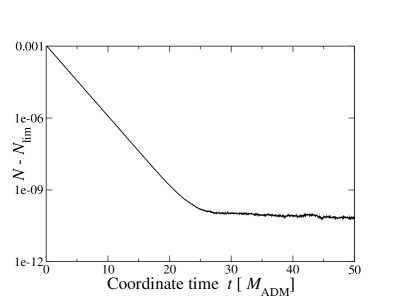
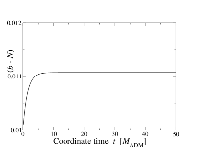
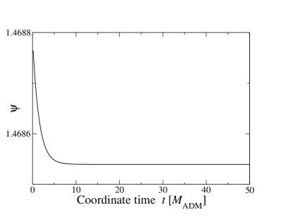
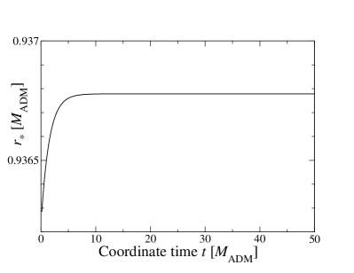
Figure 1: Evolution in terms of coordinate time $t$ of the lapse $N$, minus its time asymptotic value $N_{\rm lim}\simeq 0.549$ (left top panel, logarithmic scale); of $b$, the projection of the shift $\beta^{i}$ onto the normal to the excision surface [Eq. (19)], minus the lapse $N$ (right top panel); of the conformal factor $\psi$ (left bottom panel), at the excision surface ($r=0.916\ M_{\rm ADM}$); and of the AH coordinate radius $r_{*}$ (right bottom panel), for a spherically symmetric vacuum (i.e. Schwarzschild) BH spacetime, using excision boundary conditions described in Sec. III.2.

IV.2 Evolution of a Schwarzschild black hole

A spherically symmetric spacetime is computed for $r\geq 1$, with the previously defined boundary conditions, and the specific values $\theta^{(l)}_{0}=-0.01$, $N_{(t=0,r=1)}=0.55$ and $\left(b-N\right)_{(t=0)}=0.01$ for these initial data. Once having solved the elliptic system (7)-(9), one verifies that this setting induces a nonzero value for the Arnowitt-Deser-Misner (ADM) mass, more precisely $M_{\rm ADM}\simeq 1.09$. Numerically, it is obtained in isotropic gauge from the asymptotic behavior of the conformal factor (see e.g. Ref. FCF ),

$$M_{\rm ADM}=-\frac{1}{2\pi}\oint_{\infty}\mathcal{D}_{i}\psi\,dS^{i},$$ (32)

where the integral is taken over a sphere of radius $r\to+\infty$. This causes the excision sphere to be located at $r\simeq 0.916\ M_{\rm ADM}$. Using the numerical AH finder described in Ref. lin-07 , we have found in the initial data an AH located at the coordinate radius $r_{*}\simeq 0.94\ M_{\rm ADM}$. This is evidence that the initial data represent a BH in spherical symmetry.

This BH spacetime is then numerically evolved for $t\geq 0$, through the time integration of boundary conditions, while solving the elliptic system (7)-(9) at every given number of time steps, as described in Secs. III.2 and IV.1. This is obviously only a gauge evolution, since the spacetime is Schwarzschild by construction. The time evolution of the metric variables at the excision surface ($r=1=0.916\ M_{\rm ADM}$), namely $N$, $\psi$ and $b-N$, as well as the coordinate radius $r_{*}$ of the AH, in the interval $0\leq t\leq 50$, are displayed in Fig. 1. An exponential convergence toward stationary values is observed for all metric quantities, with an explicit behavior shown for the lapse $N$, as expected from the analysis carried out in Sec. III.3. $r_{*}$ increases with time (right bottom panel of Fig. 1), but the overall mass of the BH does not (see below).

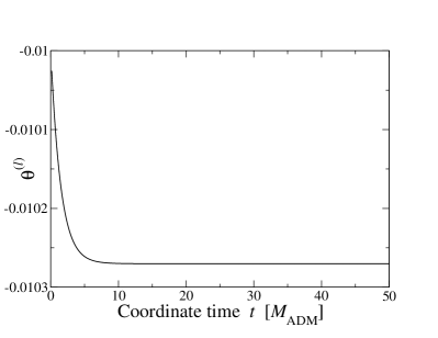
Figure 2: Evolution in terms of coordinate time $t$ of the outward expansion $\theta^{(l)}$ [Eq. (20)], for a spherically symmetric BH spacetime, as in Fig. 1.

From the top right panel of Fig. 1, one can check that the difference $b-N$ remains positive, as assumed in the discussion of Sec. III.3. The hypothesis that $(\partial_{r}\hat{\beta})|_{R}$ is negative, assumed in the same analysis of Sec. III.3, is also fulfilled during the evolution, and its value does not change significantly (the absolute value of the relative difference with respect to its initial value is $\lesssim 4\cdot 10^{-3}$). Moreover, from the formulas (29) and (30), and the computed limit in Sec. III.3 for the conformal factor at the excision boundary, one can check that the hypothesis (27) is valid; the numerically deduced value of $p$ from $\lim_{t\to\infty}\psi(t,r=1)$, and the values of $b_{0}$ and $b_{1}$, is $p\simeq 1.01$, which gives the expected behavior for the conformal factor. In Fig. 2 the time evolution of the outward expansion $\theta^{(l)}$ is displayed, which is decreasing during the simulation and always remains negative, ensuring that the excision surface always remains inside the AH.

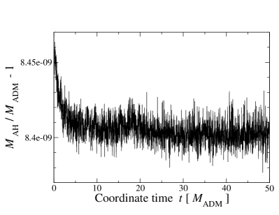
Figure 3: Evolution in terms of coordinate time $t$ of the variation of the AH irreducible mass (33) with respect to the initial ADM mass (32), for a spherically symmetric BH spacetime, using excision boundary conditions described in Sec. III.2.

The scheme appears stable (we have run it for $t\sim 1000$) and, in order to check its accuracy, we have monitored the variation of the AH irreducible mass, $M_{\rm AH}$, defined as

$$M_{\rm AH}(t)=\frac{1}{2}\sqrt{\frac{\mathcal{A}_{\rm AH}(t)}{4\pi}}=\frac{1}{2}\psi^{2}(t,r_{*}(t))\,r_{*}(t),$$ (33)

and determined by the AH finder. The Penrose inequality conjecture, in particular its rigidity part, provides a practical manner of characterizing the Schwarzschild solution. It states

$$A\leq 16\pi M_{\rm ADM}^{2}\Leftrightarrow M_{\rm AH}\leq M_{\rm ADM}\ ,$$ (34)

where the equality is valid only for slices of the Schwarzschild spacetime. The conservation of the $M_{\rm AH}$ is displayed in Fig. 3, in particular showing the numerical consistency with a Schwarzschild solution using the Penrose inequality test. The conservation of the ADM mass (32) has also been checked, with quantitatively very similar results to the conservation of the AH surface. Finally, a second-order convergence of these conserved quantities has been obtained numerically while decreasing the time step, in agreement with the implemented second-order Adams-Bashforth scheme.

The exponential convergence obtained for the chosen initial data, given by the specific values of $\theta^{(l)}_{0}$, $N_{(t=0,r=1)}>0$ and $(b-N)_{(t=0)}>0$, is independent of these initial data. A similar behavior is found for different initial values.

IV.3 Accretion of a massless scalar field

In this case we evolve a BH spacetime with energy content in the form of a minimally coupled massless scalar field in spherical symmetry; see Appendix B for details concerning the expressions of the projections of the energy-momentum tensor, the corresponding evolution equations for the scalar field and the way they are solved. Initial data are given by a Gaussian profile for the scalar field outside the excision surface, i.e. for $r\geq 1$,

$$\phi(r,t=0)=\frac{\phi_{0}r^{2}}{1+r^{2}}\,\left(e^{-(r-r_{0})^{2}/\sigma^{2}}+e^{-(r+r_{0})^{2}/\sigma^{2}}\right),$$ (35)

where $\phi_{0}$, $r_{0}$ and $\sigma$ are three constants, following e.g. Ref. alcubierre-11 . The scalar field is evolved on the numerical grid up to $r=R_{\rm max}=120\simeq 110\ M_{\rm ADM}$ (i.e. not in the compactified domain). Thus, the effect on the metric at the horizon of any scalar field wave reflected from the artificial boundary at $r=R_{\rm max}$ can be in principle neglected up to $t\sim 200$. For this simulation, we have used 24 numerical domains: one nucleus, 22 shells and a compactified domain (for details about the grid setting, see Ref. grandclement-09 ). As said, the wave equation is not solved in the compactified domain, but instead the outgoing boundary conditions (48)-(49) are imposed at $r=R_{\rm max}$. Twenty-five Chebyshev coefficients are used in each domain, in order to describe the wave accurately enough.

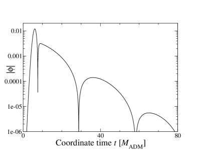
Figure 4: Evolution in terms of the coordinate time $t$ of the absolute value of the accreted scalar field, $|\phi|$, at the excision surface, $\phi(r=1,t)$.

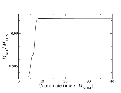
Figure 5: Evolution of the ratio between the AH irreducible mass (33) and the ADM one (32), as a function of the coordinate time $t$, for the case of the accretion of a massless scalar field.

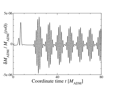
Figure 6: Evolution in terms of the coordinate time $t$ of the relative variation of the ADM mass, defined as in Eq. (32), with respect to its initial value, for the case of the accretion of a massless scalar field.

We evolve these initial data with $\phi_{0}=0.01$, $r_{0}=5$ and $\sigma=1$. A fraction of the scalar field is radiated away, while the other part is accreted onto the BH; its time evolution at the excision surface is given in Fig. 4. The metric quantities, $N$, $\beta^{r}$ and $\psi$ follow a similar evolution with respect to the vacuum case and, once the scalar field has been accreted to the BH, they settle rapidly to stationary values. Figure 5 gives the evolution of the AH mass as a function of the proper time of the observer that is located at the AH. As expected, the AH grows in time while accreting energy from the scalar field, before reaching a stationary limit. This limit does not represent all of the ADM mass of the spacetime, as part of this asymptotic mass is still contained in the scalar field traveling to higher radii. We have checked the accuracy of the code by monitoring the variation of the ADM mass, computed by Eq. (32) in Fig. 6. The conservation of this quantity, up to the level $10^{-6}$, shows that the scalar field stress-energy enters the BH and makes it grow accordingly. The first two spikes for $t\lesssim 10$ can be attributed to the scalar field which is entering the BH AH. Further oscillations that are seen in this figure for $t\gtrsim 20$ can be related to the passing of the scalar field wave from one spectral domain to another. Note that the overall level of this ADM mass violation is $10^{-6}$ and that it converges away with both time and spatial resolutions.

This simulation shows that the excision boundary conditions that have been designed here allow us to study the growth of a spherically symmetric accreting BH in a stable and accurate way.

IV.4 Collapse of a neutron star to a black hole

We here describe a simulation in spherical symmetry, starting from an unstable static neutron star, up to the formation of a BH and its accretion of all matter into the horizon. Excision is switched on during the simulation, after the AH is formed. For this simulation, we have modified the code CoCoNuT dimmelmeier-05 , so that it uses the excision technique described above, in the case of spherical symmetry. This code solves the general-relativistic Euler equations (see Appendix C for details), with Einstein’s equations in isotropic gauge. As far as hydrodynamics are concerned, in the case of grid boundary inside an AH, there is no need for boundary conditions as all the characteristics point out of the numerical integration domain (e.g. Ref. hawke-05 ). In practice, the Euler equations are solved with the use of high-resolution shock-capturing schemes (see Ref. font-08 ) and, in order to compute the fluxes at the boundary, we perform a simple copy of primitive variables into the ghost cells: the rest-mass density $\rho$, 3-velocity $v^{i}$ and internal energy $\epsilon$ (see Ref. dimmelmeier-05 for definitions). The metric equations are the same as in the previous numerical example, but with the matter sources ($E,S_{i},S_{ij}$) computed from the perfect-fluid stress-energy tensor obtained from the integration of Euler equations. Further details on the modeling of the neutron star collapse to a BH can be obtained in Ref. CC09 .

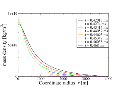
Figure 7: Radial profiles of the rest-mass density, for different moments around the start of the excision in the simulation of the collapse of a neutron star to a BH. Excision starts at $t=0.43788$ ms.

The initial data for this simulation consists of a static neutron star, computed in isotropic gauge with a polytropic equation of state of adiabatic index $\gamma_{\rm eos}=2$. The central density is such that the star lies on the unstable branch, i.e., it can either migrate toward a stable configuration with the same baryon number or collapse to a BH (see also Ref. CC09 ). The star has the following initial properties: gravitational (ADM) mass $M_{\rm ADM}=1.617~{}M_{\odot}$, baryon mass $M_{B}=1.771~{}M_{\odot}$, coordinate radius $R_{\rm star}=7.825$ km and integrated (cicular) radius $R_{\rm circ}=10.39$ km. On top of this equilibrium configuration, we have added a $1\%$ density perturbation, in order to ensure that the star collapses to a BH, and does not migrate to the stable branch.

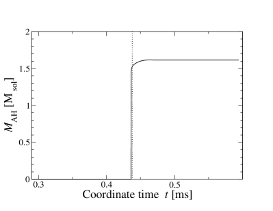
Figure 8: Evolution in terms of coordinate time $t$ of the AH irreducible mass (33) for the collapse of a neutron star to a BH. The vertical dotted line indicates the moment when excision is turned on.

The instant $t=0$ corresponds to the beginning of the collapse, which proceeds until the formation of an AH. Excision is switched on when a given ratio of the total baryon mass has entered the horizon; in practice, we have set this ratio to $85\%$, but we have checked that changing this value had little influence on the evolution of observable quantities. Note that, if this ratio is small ($\lesssim 80\%$), excision is switched on immediately after the detection of the AH. The excision radius is defined inside the AH radius $r_{*}$, with a value $r_{\rm excision}/r_{*}(t=t_{\rm excision})\in[0.9,0.98]$. Again, it has been checked that the choice for this ratio does not influence physical results. In the run shown here, $r_{\rm excision}=1329$ m. Density radial profiles at various time steps around the time when excision is started ($t=0.43788$ ms) are given in Fig. 7. In particular, the density distribution keeps a smooth behavior after the excision is switched on, and matter proceeds to fall into the BH, which reaches a stationary state, surrounded by vacuum. This is illustrated in Fig. 8, where we have plotted the time evolution of the BH irreducible mass, defined by Eq. (33). When the AH appears, it grows abruptly; the excision is then switched on and the BH accretes matter that was left outside the horizon, before settling down to the stable and stationary case. The whole simulation then remains stable, with no noticeable change in any evolved quantity.

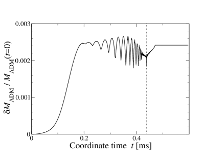
Figure 9: Evolution in terms of coordinate time $t$ of the relative variation, with respect to its initial value at $t=0$, of the ADM mass (32) for the spacetime of a neutron star collapsing to a BH. The vertical dotted line indicates the moment when excision is turned on.

We observe exponential convergence of metric quantities on the excision surface, as in Sec. IV.2, as soon as all matter has passed the excision surface. To test the accuracy of the technique, we plot the relative time variation of the ADM mass (32) of the spacetime in Fig. 9. The main error in the conservation of the ADM mass comes from the numerical solution of the Euler equations, using finite-volume methods (512 radial cells have been used). After excision has been started (dotted line in Fig. 9), this error shows a small change, and remains almost constant when the accretion phase has ended. The subsequent relative change in the ADM mass is then of the order of $10^{-8}$, similarly to Sec. IV.2. Note that the conservation of the ADM mass is not enforced in the numerical scheme, but only monitored as a global test of the accuracy of the code.

V Conclusions

In this work we have presented a new excision technique for the dynamical evolution of spherically symmetric spacetimes in the FCF in order to numerically simulate systems forming a BH.

FCF belongs to the so-called constrained formulations of Einstein’s equations, in which the constraints are solved for each time step. On the contrary, in free evolution formulations the evolution equations are in general of hyperbolic type and constraints are used to monitor the validity of the numerical solution (and/or as damping terms in the evolution scheme). The puncture method has been used in combination with the BSSN formulation for binary BH evolutions and the excision technique in combination with the generalized harmonic gauge. The difficulty of using the excision technique in the case of constrained formulations comes from the fact that constraints are elliptic-type PDEs and incorrect boundary conditions at the excision surface invalidate the physical solution in the whole numerical domain.

In the context of constrained formulations, excision has been used to generate initial data. Dynamical evolutions using constrained formulations were presented in the work of Scheel et al. scheel-95 , in the case of dust collapse in Brans-Dicke theory of gravity; in their work, the excision boundary was considered to be the AH at a fixed radial coordinate. In nonspherically symmetric spacetimes, the coordinate shape of the AH can deviate from a coordinate sphere and this approach has some limitations. In our case, as in that of Rinne and Moncrief rinne-13 , the excision boundary is a coordinate sphere located strictly inside the AH, and we let the coordinate location of the AH evolve freely in time. This approach allows in particular for a very straightforward extension to spacetimes without symmetries, where the AH can form with a shape deviating from a coordinate sphere.

The proposed approach uses an arbitrary coordinate sphere located strictly inside the AH as excision surface and a set of simple boundary conditions for the elliptic equations to be solved. It permits more freedom in the choice of the excision surface, which could be set as a simple coordinate sphere in spacetimes without symmetries. We have checked the practical applicability of this approach in three cases: the numerical simulation of a Schwarzschild spacetime, the spherically symmetric accreting BH with energy content in the form of a massless scalar field, and the collapse of a spherical neutron star to a BH. Our numerical results are stable and accurate. We have also theoretically analyzed the behavior of these boundary conditions in the proximity of stationary spacetimes and found an exponential adjustment of the coordinates to stationary values, independently of the chosen initial data. This behavior has also been checked numerically. In the last studied case, we have demonstrated that the switching on of excision during the collapse did not introduce any additional noise and that the overall simulation remained stable, with the newly formed BH accreting matter outside the excision surface. We can thus follow the whole BH formation process, from the onset of the collapse, to the growth of the BH and the description of the stationary solution up to arbitrarily long times. Although we have restricted this work to spherically symmetric spacetimes, we plan to extend this approach to more general spacetimes with less symmetries in forthcoming studies.

This excision technique can be used in the context of several astrophysical scenarios like a stellar collapse to a BH as we have shown, but also in other scenarios like the formation of an accretion disk and/or the launching of a jet. Notice that in these scenarios the initial data are usually regular, and during the simulation a BH forms and, particularly when using singularity-avoiding time coordinates (e.g. maximal slicing), an AH is found before the appearance of the physical singularity shapiro-80 . Then the excision technique can be used to continue the numerical simulation, say in the accreting period, avoiding the stretching of the grid at the center.

An advantage of this technique in combination with the use of spherical (polar) coordinates is the avoidance of the time-step limiting in the numerical simulations due to the small size of the central cells. This point can be more important for three-dimensional simulations.

Appendix A Dirac gauge and spherical symmetry

Spherical symmetry allows us to restrict the general form of the conformal metric in Eq. (4), expressed in orthonormal spherical coordinates, to

$$\tilde{\gamma}^{ij}=\left(\begin{tabular}[]{ccc}$A(r)$&0&0\\ 0&$B(r)$&0\\ 0&0&$C(r)$\end{tabular}\right),$$ (36)

with the additional determinant condition

$$A(r)\,B(r)\,C(r)=\det f^{ij}=1.$$ (37)

Equation (4) and the previous one for the determinant can be written as

$$\partial_{r}A+\frac{2A-B-C}{r}=0,\;\;B=C=\frac{1}{\sqrt{A}}$$

$$\Leftrightarrow\partial_{r}A+\frac{2(A-1/\sqrt{A})}{r}=0,\;\;B=C=\frac{1}{\sqrt{A}}.$$ (38)

A general solution for $A$ is

$$A(r)=\left(1+\frac{\omega}{r^{3}}\right)^{2/3},\;\omega\in\mathbb{R}.$$ (39)

Appendix B Massless scalar field in a curved spacetime

The massless Klein-Gordon equation, or (simply) the wave scalar equation, is given by

$$\nabla^{\mu}\nabla_{\mu}\phi=0,$$ (40)

where $\nabla$ is the Levi-Civita connection associated with the spacetime metric $g_{\mu\nu}$. The stress-energy tensor associated with this scalar field is given by

$$T_{\mu\nu}=\nabla_{\mu}\phi\nabla_{\nu}\phi-\frac{1}{2}\gamma_{\mu\nu}\nabla_{\rho}\phi\nabla^{\rho}\phi.$$ (41)

Its projections are given by

$$E = \frac{1}{2N^{2}}\left((\partial_{t}-{\cal L}_{\beta})\phi\right)^{2}+\frac{1}{2}D_{\rho}\phi D^{\rho}\phi,$$ (42)

$$S_{i} = \frac{1}{N}\left((\partial_{t}-{\cal L}_{\beta})\phi\right)D_{i}\phi,$$ (43)

$$S_{ij} = D_{i}\phi D_{j}\phi$$ (44)

$$-\frac{1}{2}\gamma_{ij}\left[D_{k}\phi D^{k}\phi-\frac{1}{N^{2}}\left((\partial_{t}-{\cal L}_{\beta})\phi\right)^{2}\right],$$

where $D$ is the Levi-Civita connection associated with the spatial metric $\gamma_{ij}$.

The wave equation (40) is rewritten as a first-order system in space and time, by introducing the auxiliary scalar $\Pi$, defined from Eq. (45) below, and the vector $\Phi_{i}={\cal D}_{i}\phi$, considered also as a constraint of the system, as

$$\partial_{t}\phi = -N\,\Pi+\beta^{i}{\cal D}_{i}\phi,$$ (45)

$$\partial_{t}\Pi = -N\,\gamma^{ij}\,{\cal D}_{i}\Phi_{j}+\beta^{i}{\cal D}_{i}\Pi$$ (46)

$$-\frac{\Phi_{i}{\cal D}_{j}(N\psi^{6}\gamma^{ij})}{\psi^{6}}+\Pi NK,$$

$$\partial_{t}\Phi_{i} = -{\cal D}_{i}(N\,\Pi)+\Phi_{k}{\cal D}_{i}\beta^{k}+\beta^{k}{\cal D}_{k}\Phi_{i}.$$ (47)

This system is solved using a second-order Adams-Bashforth scheme, with the time step being a submultiple of the one used for the evolution of the boundary conditions for the metric. Note that, in the case of the maximal slicing condition $(K=0)$, the last term of Eq. (46) vanishes.

Matching across different domains is done along characteristic fields, in an upwind manner. At the outer boundary ($r=R_{\rm max}$), before the compactified domain, we impose a Sommerfeld-like condition,

$$\partial_{t}\left(\Pi-\Phi_{r}\right)_{r=R_{\rm max}}=0,$$ (48)

and the consistency condition for $\phi$,

$$\left.\partial_{t}\phi\right|_{r=R_{\rm max}}=\left(-N\Pi+\beta^{r}\Phi_{r}\right)_{r=R_{\rm max}}.$$ (49)

No boundary condition is needed for either field at the inner boundary (excision at $r=0.916\ M_{\rm ADM}$),as all characteristics are directed out of the computational domain as long as the excision surface is spacelike, which is verified in our case with $b-N>0$ in our numerical simulations. All matching and boundary conditions are implemented in a collocation approach to spectral variables.

Appendix C Perfect-fluid equations

Einstein’s equations, in the case of nonvacuum spacetimes, have to be solved coupled with the hydrodynamic equations for the evolution of matter which can be derived from the local conservation of baryon number and energy-momentum, respectively,

$$\nabla_{\mu}J^{\mu}=0,\;\;\nabla_{\mu}T^{\mu\nu}=0,$$ (50)

with the current $J^{\mu}$ and the energy momentum-tensor $T^{\mu\nu}$ of a perfect fluid being

$$J^{\mu}=\rho\,u^{\mu},\;\;T^{\mu\nu}=\rho\,h\,u^{\mu}\,u^{\nu}+p\,g^{\mu\nu},$$ (51)

where $\rho$ is the rest-mass (baryon mass) density, $u^{\mu}$ is the 4-velocity of the fluid, $h=1+\epsilon+p/\rho$ is the specific enthalpy, $\epsilon$ is the specific internal energy and $p$ is the pressure. The previous system of equations (50) can be written as a first-order hyperbolic system for the conserved variables $(D,S^{j},\tau)=(\rho\,W,\rho\,h\,W\,v^{j},\rho\,h\,W^{2}-p-\rho\,W)$, with $W$ being the Lorentz factor font-08 .

References

- (1) F. Pretorius, Phys. Rev. Lett. 95, 121101 (2005).
- (2) M. Campanelli, C.O. Lousto, P. Marronetti, and Y. Zlochower, Phys. Rev. Lett. 96, 111101 (2006).
- (3) J.G. Baker, J. Centrella, D.-I. Choi, M. Koppitz, and J. van Meter, Phys. Rev. Lett. 96, 111102 (2006).
- (4) E. Seidel and W.-M. Suen, Phys. Rev. Lett. 69, 1845 (1992).
- (5) L. Lehner, M. Huq, M. Anderson, E. Bonning, D. Schaefer, and R. Matzner, Phys. Rev. D 62, 044037 (2000).
- (6) S. Brandt and B. Brügmann, Phys. Rev. Lett. 78, 3606 (1997).
- (7) M. Hannam, S. Husa, D. Pollney, B. Brügmann, and N. Ó Murchadha, Phys. Rev. Lett. 99, 241102 (2007).
- (8) M. Boyle, D.A. Brown, L.E. Kidder, A.H. Mroué, H.P. Pfeiffer, M.A. Scheel, G.B. Cook, and S.A. Teukolsky, Phys. Rev. D 76, 124038 (2007).
- (9) T.W. Baumgarte and S.L. Shapiro, Phys. Rev. D 59, 024007 (1999).
- (10) M. Shibata and T. Nakamura, Phys. Rev. D 52, 5428 (1995).
- (11) E.N. Dorband, E. Berti, P. Diener, E. Schnetter and M. Tiglio, Phys. Rev. D 74, 084028 (2006).
- (12) S. Bonazzola, E. Gourgoulhon, P. Grandclément, and J. Novak, Phys. Rev. D 70, 104007 (2004).
- (13) J.L. Jaramillo, E. Gourgoulhon, I. Cordero-Carrión, and J.M. Ibáñez, Phys. Rev. D 77, 047501 (2008).
- (14) G.B. Cook and H.P. Pfeiffer, Phys. Rev. D 70, 104016 (2004).
- (15) J.L. Jaramillo, E. Gourgoulhon, and G.A. Marugán, Phys. Rev. D 70, 124036 (2004).
- (16) S. Dain, J.L. Jaramillo, and B. Krishnan, Phys. Rev. D 71, 064003 (2005).
- (17) E. Gourgoulhon and J.L. Jaramillo, Phys. Rep. 423, 159 (2006).
- (18) M. Caudill, G.B. Cook, J.D. Grigsby, and H.P. Pfeiffer, Phys. Rev. D 74, 064011 (2006).
- (19) J.L. Jaramillo, Phys. Rev. D 79, 087506 (2009).
- (20) J.L. Jaramillo, M. Ansorg, and F. Limousin, Phys. Rev. D 75, 024019 (2007).
- (21) N. Vasset, J. Novak, and J.L. Jaramillo, Phys. Rev. D 79, 124010 (2009).
- (22) S.L. Shapiro and S.A. Teukolsky, Astrophys. J. 235, 199-215 (1980).
- (23) B. Peres, M. Oertel and J. Novak, Phys. Rev. D 87, 043006 (2013).
- (24) K. Nakazato, S. Furusawa, K. Sumiyoshi, A. Ohnishi, S. Yamada and H. Suzuki, Astrophys. J. 745, 197 (2012).
- (25) E. O’Connor and C.D. Ott, Astrophys. J. 730, 70 (2011).
- (26) M.A. Scheel, S.L. Shapiro and S.A. Teukolsky, Phys. Rev. D 51, 4208 (1995).
- (27) O. Rinne and V. Moncrief, Classical Quantum Gravity 30, 095009 (2013).
- (28) I. Cordero-Carrión, J.M. Ibáñez, E. Gourgoulhon, J.L. Jaramillo, and J. Novak, Phys. Rev. D 77, 084007 (2008).
- (29) I. Cordero-Carrión, P. Cerdá-Durán, H. Dimmelmeier, J.L. Jaramillo, J. Novak, and E. Gourgoulhon, Phys. Rev. D 79, 024017 (2009).
- (30) I. Cordero-Carrión, P. Cerdá-Durán, and J.M. Ibáñez, Phys. Rev. D 85, 044023 (2012).
- (31) I. Cordero-Carrión, J.M. Ibáñez, and J.A. Morales-Lladosa, J. Math. Phys. 52, 112501 (2011).
- (32) A. Arbona, C. Bona, J. Carot, L. Mas, J. Massó and J. Stela, Phys. Rev. D 57, 2397 (1998).
- (33) D. Brown, O. Sarbach, E. Schnetter, M. Tiglio, P. Diener, I. Hawke and D. Pollney, Phys. Rev. D 76, 081503 (2008).
- (34) D.A. Hemberber, M.A. Scheel, L.E. Kidder, B. Szilágyi, G. Lovelace, N.W. Taylor and S.A. Teukolsky, Classical Quantum Gravity 30, 115001 (2013).
- (35) J.L. Jaramillo, Int. J. Mod. Phys. D 20, 21692204 (2011).
- (36) S.A. Hayward, Phys. Rev. D 49, 6467 (1994).
- (37) I. Booth, L. Brits, J.A. Gonzalez and C. Van Den Broeck, Classical Quantum Gravity 23, 413 (2006) [gr-qc/0506119].
- (38) I. Cordero-Carrión and J.L. Jaramillo, in CoCoNuT Meeting 2009, Valencia, Spain, 2009, www.mpa-garching.mpg.de/hydro/COCONUT/Valencia2009/Talks/Cordero-Carrion.pdf
- (39) R.L. Marsa and M.W. Choptuik, Phys. Rev. D 54, 4929 (1996).
- (40) http://www.lorene.obspm.fr
- (41) P. Grandclément and J. Novak, Living Rev. Relativity 12, 1 (2009).
- (42) L.-M. Lin and J. Novak, Classical Quantum Gravity 24, 2665 (2007).
- (43) M. Alcubierre and M.D. Mendez, Gen. Relativ. Gravit. 43, 2769 (2011).
- (44) H. Dimmelmeier, J. Novak, J.A. Font, J.M. Ibáñez and E. Müller, Phys. Rev. D 71, 064023 (2005).
- (45) I. Hawke, F. Löffler and A. Nerozzi, Phys. Rev. D 71, 104006 (2005).
- (46) J.A. Font, Living Rev. Relativity 11, 7 (2008).