Asymptotic solutions in f(R)-gravity

Abstract

We study cosmological solutions in $R+\beta R^{N}$-gravity for an isotropic Universe filled with ordinary matter with the equation of state parameter $\gamma$. Using the Bogolyubov-Krylov-Mitropol’skii averaging method we find asymptotic oscillatory solutions in terms of new functions, which have been specially introduced by us for this problem and appeared as a natural generalization of the usual sine and cosine. It is shown that the late-time behaviour of the Universe in the model under investigation is determined by the sign of the difference $\gamma-\gamma_{crit}$ where $\gamma_{crit}=2N/(3N-2)$. If $\gamma<\gamma_{crit}$, the Universe reaches the regime of small oscillations near values of Hubble parameter and matter density, corresponding to General Relativity solution. Otherwise higher-curvature corrections become important at late times. We also study numerically basins of attraction for the oscillatory and phantom solutions, which are present in the theory for $N>2$. Some important differences between $N=2$ and $N>2$ cases are discussed.

1 Introduction

Theories of modified gravity (see [1] for a review), motivated initially from Quantum Field Theory recently became a matter of intense investigation mainly in order to describe the observed accelerated expansion of our Universe ([2],[3]). It has been shown that one of the simplest modified gravity theories, $f(R)$ gravity can, in principle, explain this experimental fact without any need of exotic matter, though it appeared to be rather tricky and requires a specially designed (often without any background physical motivation) form of the function $f$ (see [4]-[6] and also reviews on $f(R)$ gravity [7]-[12]). On the other hand, detailed studies of cosmological dynamics in $f(R)$ theories have revealed existence of cosmological regimes, which are absolutely incompatible with the picture of Universe we live in. For example, any theory with power-law $f(R)=R+\beta R^{N}$ with $N>2$ has a solution containing a ”Big Rip” singularity (see [13, 14, 15, 16, 17, 18, 19, 20, 21, 22, 23, 24, 25, 26] for ”Big Rip” singularities and [27, 28, 29, 30, 31, 32, 33] for their presence in $R^{N}$ gravity and some extensions).

Keeping this in mind it is reasonable to go back to the initial motivation and formulate a problem: if we assume that some quantum considerations lead to $f(R)$ theory in a high-energy regime, can we be sure that such corrections to Einstein gravity do not spoil well-established facts about cosmological evolution?

As a general $f(R)$ theory has an additional degree of freedom (dubbed as a scalaron in [34]), it is natural to expect that a solution close to Einstein gravity should be oscillations near the General Relativity (GR) solution. It is known that for $R+\beta R^{2}$ theory the effects coming from quadratic curvature corrections can be represented as an effective massive scalar field, so cosmological dynamics can be considered as a combination of a smooth evolution and harmonic oscillations imposed on it. Dynamics in $R+\beta R^{2}$ theory depends on the equation of state for matter, filling the Universe,

$$p=({\gamma{}}-1)\rho\,,\quad\text{where $p$ is pressure and $\rho$ is an energy density.}$$

If the equation of state parameter $\gamma<1$, the smooth part of solution coincides with GR behaviour, otherwise the influence of quadratic curvature correction becomes important at late times (see [35, 36]).

This work is devoted to asymptotic oscillatory solutions in general $R+\beta R^{N}$–gravity, which can be relevant for the description of reheating phase after inflation (see [43, 44, 45] for inflation in $R^{N}$–gravity). A general power-law case differs from $N=2$ case in several points. First, the oscillations become anharmonic and can not be represented in elementary functions. Second, the Big Rip solution absent in the case of $N=2$ appears for any $N>2$. In the present paper we address both problems. Using analytical methods we will describe oscillations and find a critical value of $\gamma$ as a function of $N$, generalizing the $\gamma=1$ condition known for $N=2$ to arbitrary $N>1$. After, we use numerics to find a region in the initial conditions space starting from which a trajectory indeed reaches an oscillatory regime and do not fall into a Big Rip singularity.

It should be pointed out that in $R+\beta R^{2}$ gravity the mentioned oscillations of $R$ lead to gravitational creation of particles and prevent an overproduction of scalarons ([34]). However, in the case of $R+\beta R^{N}$ this mechanism can not be applied since it is unclear how to evolve through the point $f^{\prime\prime}(R)=0$, where the sclaron rest mass diverges ([40]). This issue has another face, called ”non-standard singularity”, taking place when a coefficient in front of a higher derivative in the equations of motion (which is proportional to $f^{\prime\prime}(R)$) vanishes. We will find this problem in our research and propose a technique to avoid such a difficulty at least at the level of background dynamics. Note, that in this paper we do not consider energy exchange between scalaron and ordinary (including Dark) matter. In realistic models where the inflation is driven by higher–order terms, this interaction is necessary for a reheating when the scalaron decays into Dark Matter and Standard Model particles ([41],[42]).

Apart from the technique using in our study, many other analytical methods have been recently applied to $R^{N}$ gravity ([30],[37],[38]). Small oscillations near several GR solutions have been studied in [39], however, our approach allows to describe oscillations in the regime where corrections to GR can not be considered as small and can even dominate GR dynamics.

Our work is organized as follows. In the section (2) we present the model and discuss its asymptotic behaviour in the Einstein frame. Section (3) contains the analytic study of dynamical equations in the Jordan frame in the limit of weak couplings of $R^{N}$ term in the action. In the subsections (3.1-3.2) we prepare the equations of motion for the Bogolyubov-Krylov-Mitropol’skii averaging procedure and apply it in the subsection (3.3). The reader, who is not interested in technicalities may go directly to the subsection (3.4) containing main analytic results. In the section (4) we discuss what happens in the case of strong couplings, where the analytical scheme breaks down. Section (5) contains summary of our results. Finally, in the Appendix (A) we present a systematic treatment of generalised trigonometric functions, used in (3).

2 The model and a picture in the Einstein frame

The action we study is given in the Jordan frame by

$$S^{JF}=\int d^{4}x\,\sqrt{-g}\frac{f(R)}{6}+S_{matter}^{JF}(g^{\mu\nu},\varphi_{i}),$$ (1)

where $S_{matter}$ is the action for matter fields $\varphi_{i}$ universally coupled to the metric. It is well-known that $f(R)$-gravity is classically equivalent to the scalar-tensor gravity via the Legendre-Weyl transformation [47]. Let us firstly discuss the picture in the Einstein frame; it will help us to understand qualitatively an asymptotic behaviour in the considered theory. Performing a standard transition to the Einstein frame (see for instance [8]) and introducing a scalar degree of freedom (scalaron hereafter) through

$$f^{\prime}(R)=\exp{[\sqrt{2}\phi]}\,,\quad\text{where}\quad f^{\prime}\equiv\partial f/\partial R\,,$$ (2)

one writes down an equivalent action in the form

$$S^{EF}=\int d^{4}x\,\sqrt{-g_{E}}\,\left[\frac{R_{E}}{6}-\frac{1}{2}g^{\mu\nu}\partial_{\mu}\phi\partial_{\nu}\phi-V(\phi)\right]+S_{matter}^{EF}(g^{\mu\nu}_{E},\varphi_{i},\phi)\,,$$ (3)

where the subscript $E$ corresponds to quantities in the Einstein frame. Notice that the scalaron $\phi$ now couples to the matter fields. In the present paper we study the simplest $f(R)$ theory, namely $R+\beta R^{N}$. This theory has been well-investigated in the Einstein frame in the context of inflationary dynamics ([43, 44, 45]). The scalaron potential in the chosen unit system (footnote 5) has the following form,

$$V(\phi)=V_{0}(1-e^{-\sqrt{2}\phi})^{\frac{N}{N-1}}e^{-\frac{N-2}{N-1}\sqrt{2}\phi},\quad\text{where}\quad V_{0}\equiv\frac{N-1}{6N}\left(\frac{1}{\beta N}\right)^{\frac{1}{N-1}}\,,$$ (4)

and is plotted on the graph (1) for a set of parameters $N$.

Figure 1: Scalaron potential (4) in the Einstein frame for the function $f(R)=R+\beta R^{N}$.

We clearly see that the case of $N=2$ (Starobinsky model) sufficiently differs from other cases of $N$. The potential for Starobinsky model has smooth non-zero constant asymptotic in the limit $\phi\to\infty$, while for other cases of $N$ we have a runaway potential. As a consequence, the theory with $N>2$ exhibits stable singular behaviour, mentioned in the introduction. From the shape of the potential it is clear that if the scalaron is at the right sight of the potential maxima, then it would roll down into the area $\phi\to\infty$. Such behaviour of the scalaron can be translated into terms of curvature in the Jordan frame via (2),

$$\phi=2^{-1/2}\ln{f^{\prime}}=2^{-1/2}\ln{(1+N\beta R^{N-1})}\to\infty,$$

implying $R\to\infty$, what indeed represents the known Big Rip singularity of $R^{N}$-gravity.

In the present paper we are going to investigate attractor solutions (i.e. stable regimes occurred at late times) in the general $R+\beta R^{N}$ theory. From the Fig.1 it is evident that for $N=2$ we have the only oscillating solution near the minimum of the potential while for $N>2$ two regimes are possible: either scalaron falls into the minimum of the potential and oscillate there, or rolls down into the unrestricted area located to the right from the maximum of the potential. We will describe analytically the oscillatory solution for arbitrary $N$ and generalize the results obtained for the Starobinsky model. After, we will specify which initial conditions lead to the mentioned above two different behaviours. We choose to work in the Jordan frame for two reasons. First, it is more related to the observations ([46]) and second for the sake of relative simplicity, since the cosmological dynamics in the Einstein frame for the non-vacuum case appeared to be more complicated than the dynamics in the Jordan frame due to presence of a scalaron-matter coupling.

3 The case of weak couplings: analytical study

In this section we consider the case of $\beta\ll 1$, leaving the strong coupling limit $\beta\sim 1$ for the next section. The chosen case allows us to study the model analytically and find asymptotic oscillatory solution.

Varying the action (1) on metric we write down the (00)-equation of motion in $f(R)$-gravity for the flat Friedmann-Lemaitre-Robertson-Walker (FLRW) Universe filled with matter with the energy density $\rho$ and the pressure $p=(\gamma-1)\rho$ :

$$3f^{\prime}H^{2}=(f^{\prime}R-f)/2-3H\dot{f^{\prime}}+3\rho\,,$$ (5)

supplemented by the Ricci scalar expression and the continuity equation:

$$R=6(2H^{2}+\dot{H})\,,$$ (6)

$$\dot{\rho}+3H\gamma\rho=0\,.$$ (7)

Using $\dot{f^{\prime}}=f^{\prime\prime}\dot{R}$, the eq.(5) may be resolved with respect to the higher derivative

$$18f^{\prime\prime}(H,\dot{H})H\ddot{H}=\frac{1}{2}(f^{\prime}-fR)-3f^{\prime}H^{2}-72f^{\prime\prime}H^{2}\dot{H}\,+3\rho.$$ (8)

We intend to study the power-law theory $f(R)=R+\beta R^{N}$. Looking at eq. (8) one sees that if the scalar curvature $R$ change its sign, the coefficient $f^{\prime\prime}$ in front of the higher derivative $\ddot{H}$ in the case of odd $N$ also change its sign, providing so-called ”non-standard singularity” (see discussion below). To prevent this we insert a modulus in our definition of $f(R)$:

$$f(R)=R+\beta|R|^{N}\,,\quad f^{\prime}=1+\beta N|R|^{N-1}(\text{sign}R)\,.$$

Generally speaking, the power index may have any value $N>1$ (including non-integer). The (00)-equation then can be rewritten as:

$$H^{2}=\rho+\frac{\beta(N-1)}{6}|R|^{N-2}\left[R^{2}-\frac{6N}{N-1}H^{2}R-6HN\dot{R}\right]\,\equiv\rho+\beta\rho_{f(R)}\,.$$ (9)

The sign of coupling $\beta$ is fixed to be positive by the stability conditions $f^{\prime}>0,f^{\prime\prime}>0$ ([48, 49, 50]), which also exclude the case of $N<1$ from our consideration. In general the eq. (9) is a non-linear second order differential equation, which is impossible to solve explicitly. However, in the case of small coupling $\beta$ in front of the higher derivative term, one can find an asymptotic solution (with respect to the constant $\beta$). Introducing some useful notations:

$$\varepsilon^{N}\equiv(N-1)6^{N-1}\beta\,,\quad R=\frac{6Q}{\varepsilon}\,,$$

$$\tau=\frac{t-t_{0}}{\varepsilon}\quad\Rightarrow\quad t=t_{0}+\varepsilon\tau\,,$$ (10)

we find the following expression for the second term in eq.(9):

$$\beta\rho_{f(R)}=-|Q|^{N-2}(NHQ_{\tau}-Q^{2}+\frac{N}{N-1}\varepsilon H^{2}Q)\,\quad\text{where}\quad Q_{\tau}\equiv\frac{dQ}{d\tau}\,.$$ (11)

Finally, collecting eqs. (6,7,9) one finds the following system of equations:

$$H_{\tau} =Q-2\varepsilon H^{2}\,,$$ (12a)

$$NH|Q|^{N-2}Q_{\tau} =|Q|^{N}+\rho-H^{2}-\frac{N}{N-1}\varepsilon H^{2}Q|Q|^{N-2}\,,$$ (12b)

$$\rho_{\tau} =-3\varepsilon\gamma H\rho\,.$$ (12c)

General solution of this system as well as its integrals (finite expressions, defining a solution implicitly) can not be expressed in quadratures. Our goal is to find an asymptotic (regarding the small parameter $\varepsilon$) approximate solution, i.e. the solution with a precision, growing unlimitedly with $\varepsilon$ tending to zero.

Let us discuss our strategy. We intend to find an asymptotic solution of the system (12) using the Krylov-Bogolyubov-Mitropol’skii averaging method ([52]). To do that one should change variables and transform initial equations to the so-called standard form, which may be of the two different variates: either the usual one or the system with rapidly rotating phase [51]. We will find that the last one is the case for our model; the resulting system will take a form

$$\Bigg{\{}\begin{aligned} \textbf{x}_{t}&={\bf X}(\textbf{x},\psi,\varepsilon)\,,\\ \psi_{t}&=\varepsilon^{-1}\omega(\textbf{x})+\Psi({\bf x},\psi,\varepsilon)\,,\end{aligned}$$ (13)

where $\bf{X}$,$\Psi$ are periodic functions of the phase $\psi$ and $\textbf{x}=(x,y)$ is a vector of new variables. In this system variables $\bf{x}$ are ”slow” in the sense that ${x}_{t}\sim 1$, ${y}_{t}\sim 1$ and the variable $\psi$ is ”rapid” because $\psi_{t}\sim\varepsilon^{-1}\gg 1$. Thus for one period of oscillations the functions $\bf{X}$,$\Psi$ change slowly in comparison with the changing rate of $\psi$, which allows us to average $\bf{X}$,$\Psi$ with respect to $\psi$. The presence of a large parameter in the r.h.s of a dynamical equation can be considered as a definition for systems with rapidly rotating phase (see the excellent monograph [51] for more details). If it is not the case and the system contains only ”slow” variables, then it has the so-called usual standard form just as the first line of (13).

To find a proper form of a transformation, we put $\varepsilon=0$ in all the equations (12) and obtain a general unperturbed solution. At the next step we vary integration constants of the unperturbed solution and use them as new variables $\bf{x}$ for the problem (13). At the final step we solve the system (13) by the averaging method.

3.1 General solution of the unperturbed system

Following the proposed algorithm, we consider the unperturbed regular system:

$$\rho_{\tau} =0\,,$$ (14a)

$$H_{\tau} =Q\,,$$ (14b)

$$NH|Q|^{N-2}Q_{\tau} =|Q|^{N}+\rho-H^{2}\,.$$ (14c)

A solution of the system (14) can not be found explicitly as before, but one may find its integrals, i.e. some expressions containing $H,Q$ and $\rho$, defining solution implicitly. Solving the first equation (14a) one immediately finds

$$\rho =\text{const}\equiv C_{2}\,,$$ (15a)

$$H_{\tau} =Q\,,$$ (15b)

$$NH|Q|^{N-2}Q_{\tau} =|Q|^{N}+C_{2}-H^{2}\,.$$ (15c)

Let us multiply eq. (15c) on $Q$ and divide by $H^{2}$ (which always has non-zero value):

$$\frac{N|Q|^{N-2}QQ_{\tau}}{H}-\frac{|Q|^{N}Q}{H^{2}}=\frac{C_{2}Q}{H^{2}}-Q$$ (16)

Note, that the numerator of the first fraction is exactly $d|Q|^{N}/d\tau$:

$$(|Q|^{N})_{\tau}=N|Q|^{N-1}|Q|_{\tau}=N|Q|^{N-2}(Q\,\text{sign}Q)(Q\,\text{sign}Q)_{\tau}=N|Q|^{N-2}QQ_{\tau}.$$ (17)

Next, dividing (15b) on $H^{2}$,

$$\frac{Q}{H^{2}}=\frac{H_{\tau}}{H^{2}}=\left(-\frac{1}{H}\right)_{\tau}\,,$$ (18)

and using eqs. (16,17) one obtains:

$$(|Q|^{N})_{\tau}\left(\frac{1}{H}\right)+(|Q|^{N})\left(\frac{1}{H}\right)_{\tau}=-C_{2}\left(\frac{1}{H}\right)_{\tau}-H_{\tau}\,,$$ (19)

leading to the new integral of motion:

$$\frac{|Q|^{N}}{H}+H+\frac{C_{2}}{H}=C=2C_{1}\,.$$ (20)

Using (15b) and performing some simple algebraic actions, one finds the first-order equation for $H$:

$$|H_{\tau}|^{N}+(H-C_{1})^{2}=C_{1}^{2}-C_{2}\,.$$ (21)

To obtain a solution of this equation one has to solve an inversion problem for elliptic ($N=3,4$) or hyperelliptic ($N>4$) integrals [63], i.e. one has to find corresponding inverse functions. However, in doing so the solution of (21) (in terms of mentioned inverse functions) can not be expressed neither in elliptical nor in elementary functions (except the cases of $N=2$ and $C_{1}^{2}-C_{2}=0$). To proceed we have defined and studied properties of new functions, describing the solution; these functions appeared to be a natural generalisation of usual trigonometric sine and cosine. The reader may find all the details in the Appendix (A); in the main text we just present the final solution of the unperturbed system:

$$H =H(C_{1},C_{2},\psi)\equiv C_{1}+\sqrt{C_{1}^{2}-C_{2}}\sin_{N}(\psi)\,,$$ (22a)

$$Q =Q(C_{1},C_{2},\psi)\equiv\operatorname{Sg}_{N}(\psi)\sqrt[N]{C_{1}^{2}-C_{2}}\sqrt[N]{1-\sin^{2}_{N}(\psi)}\,,$$ (22b)

$$\rho =\rho(C_{1},C_{2},\psi)\equiv C_{2}\,,$$ (22c)

where the function $\sin_{N}(\psi)$ is defined in (Def. 1, 94) and

$$\psi \equiv(C_{1}^{2}-C_{2})^{\frac{2-N}{2N}}\tau+\text{const}\,,$$ (23)

$$\operatorname{sign}\sin^{\prime}_{N}(\psi) =\operatorname{sign}Q(\tau)\equiv\operatorname{Sg}_{N}(\psi)\,.$$ (24)

From (23) one observes the appearance of a ”rapid phase”. For $N\neq 2$ the phase $\psi$ depends on the integration constants which we are going to vary according to the Bogolyubov-Krylov procedure. As a result, $\psi_{\tau}$ will stop to be a constant, $\psi_{\tau}=\psi_{\tau}(C_{1}(\tau),C_{2}(\tau),C_{1}(\tau)_{\tau},C_{2}(\tau)_{\tau},\tau)\neq\text{const}$; and after proper transformations presented below it will take a form of the second line in the Eqs.(13).

3.2 Transformation to the system with rapidly rotating phase

To solve the perturbed system (12) let us vary the constants $C_{1},C_{2}$ with respect to the time and define $C_{1}=x(\tau),C_{2}=y(\tau)$ . The solution of (22) then reads:

$$H =H(C_{1},C_{2},\psi)\equiv x+\sqrt{x^{2}-y}\sin_{N}(\psi)\,,$$ (25a)

$$Q =Q(C_{1},C_{2},\psi)\equiv\operatorname{Sg}_{N}(\psi)\sqrt[N]{x^{2}-y}\sqrt[N]{1-\sin^{2}_{N}(\psi)}\,,$$ (25b)

$$\rho =\rho(C_{1},C_{2},\psi)\equiv y\,.$$ (25c)

As it has been discussed, $x(\tau),y(\tau),\psi(\tau)$ are new variables for the problem (13). Now let us transform the system (25) to the dynamical system for $x,y,\psi$, i.e. let us get equations for $x_{\tau},\psi_{\tau}$ (an equation for $y_{\tau}$ is already obtained, see (12c)). Performing a simple differentiating of the function $Q(H,x,y)=\operatorname{Sg}_{N}(\psi)\sqrt[N]{x^{2}-y-{(H-x)}^{2}}$,

$$Q_{\tau} =Q_{H}\,H_{\tau}+Q_{x}\,x_{\tau}+Q_{y}\,y_{\tau}=\frac{2}{N}\,\frac{x-H}{{|Q|}^{N-2}}+\frac{2}{N}\,\frac{H\,x_{\tau}}{{|Q|}^{N-2}\,Q}-\frac{1}{N}\,\frac{y_{\tau}}{{|Q|}^{N-2}\,Q}-\frac{4}{N}\,\varepsilon\,\frac{(x-H)\,H^{2}}{{|Q|}^{N-2}\,Q}\,,$$

where we defined lower subscripts as

$$z_{\tau}\equiv\frac{d}{d\tau}z\,,\quad z_{j}\equiv\frac{\partial}{\partial j}z\,,\quad j=(\psi,x,y)\,,$$

and taking into account the eqs. (12b,12c) one finds the following expression for $x_{\tau}$:

$$x_{\tau}={}-2\,\varepsilon\,(x^{2}-y)+\tfrac{3\,N-4}{2\,(N-1)}\,\varepsilon\,(x^{2}-y)\,(1-\sin^{2}_{N}(\psi))-2\,\varepsilon\,x\,\sqrt{x^{2}-y}\,\sin_{N}(\psi){}-\tfrac{3}{2}\,\varepsilon\,{\gamma{}}\,y\,.$$

Using the eq.(12a) we write down

$$H_{\tau}=H_{x}\,x_{\tau}+H_{y}\,y_{\tau}+H_{\psi}\,\psi_{\tau}\ =\,Q\,=\sqrt[N]{x^{2}-y}\,\sin^{\prime}_{N}(\psi)=H_{\psi}\,{(x^{2}-y)}^{\frac{2-N}{2N}}\,,$$ (26)

$$\text{and express}\quad\psi_{\tau}={(x^{2}-y)}^{\frac{2-N}{2N}}-\frac{H_{x}}{H_{\psi}}\,x_{\tau}-\frac{H_{y}}{H_{\psi}}\,y_{\tau}-2\,\varepsilon\,\frac{H^{2}}{H_{\psi}}\,.$$ (27)

Looking at (25,97) we calculate partial derivatives $H_{x},H_{y},H_{\psi}$:

$$H_{x}\,x_{\tau}+H_{y}\,y_{\tau}+2\,\varepsilon\,H^{2}={}-\frac{\varepsilon}{2(N-1)}\,\Big{\{}-(1-\sin^{2}_{N}(\psi))\,\Big{[}(3\,N-4)\,x^{2}+(N-3\,(N-1)\,{\gamma{}})\,y\\ +(3\,N-4)\,x\,\sqrt{x^{2}-y}\,\sin_{N}(\psi)\Big{]}\Big{\}}\,,$$ (28)

and plug them into the eq. (27):

$$\psi_{\tau}={(x^{2}-y)}^{\frac{2-N}{2N}}-\frac{\varepsilon}{2\,(N-1)}\,\frac{\operatorname{Sg}_{N}(\psi)}{\sqrt{x^{2}-y}}\,\Big{[}(3\,N-4)\,x^{2}+(N-3\,(N-1)\,{\gamma{}})\,y+{}\\ {}+(3\,N-4)\,x\,\sqrt{x^{2}-y}\,\sin_{N}(\psi)\Big{]}\,{(1-\sin^{2}_{N}(\psi))}^{\frac{N-1}{N}}\,.$$

Going back to the standard physical time $t$,

$$\tau=\frac{t-t_{0}}{\varepsilon},\quad t=t_{0}+\varepsilon\,\tau,\quad dt=\varepsilon\,d\tau\,,$$

we obtain the resulting dynamical system to solve:

$$x_{t} =\begin{aligned} {}-2\,(x^{2}-y)+\tfrac{3\,N-4}{2\,(N-1)}\,(x^{2}-y)\,[1-\sin^{2}_{N}(\psi)]-2\,x\,\sqrt{x^{2}-y}\,\sin_{N}(\psi)-\tfrac{3}{2}\,{\gamma{}}\,y\equiv\\ \equiv X_{0}(x,y,\psi),\end{aligned}$$ (29a)

$$y_{t} ={}-3\,{\gamma{}}\,x\,y-3\,{\gamma{}}\,y\,\sqrt{x^{2}-y}\,\sin_{N}(\psi)\equiv Y_{0}(x,y,\psi),$$ (29b)

$$\psi_{t} =\begin{aligned} &\varepsilon^{-1}\,{(x^{2}-y)}^{\frac{2-N}{2N}}-\tfrac{1}{2\,(N-1)}\,\tfrac{(3\,N-4)\,x^{2}+(N-3\,(N-1)\,{\gamma{}})\,y}{\sqrt{x^{2}-y}}\,{[1-\sin^{2}_{N}(\psi)]}^{\frac{N-2}{N}}\sin^{\prime}_{N}(\psi)-{}\\ &{}-\tfrac{3\,N-4}{2\,(N-1)}\,x\,\sqrt{x^{2}-y}\,\sin_{N}(\psi)\,{[1-\sin^{2}_{N}(\psi)]}^{\frac{N-2}{N}}\sin^{\prime}_{N}(\psi)\equiv\varepsilon^{-1}\,\omega(x,y)+\Psi_{0}(x,y,\psi)\,,\end{aligned}$$ (29c)

where

$$x=x(t,\varepsilon),\quad y=y(t,\varepsilon),\quad\psi=\psi(t,\varepsilon).$$

The functions $X_{0}(x,y,\psi)$, $Y_{0}(x,y,\psi)$ and $\Psi_{0}(x,y,\psi)$ are periodic with respect to $\psi$ with the same period $T_{0}$ as $\sin_{N}(\psi)$(99). The essential fact is that the function at $\varepsilon^{-1}$ in the r.h.s. of (29c),

$$\omega(x,y)={(x^{2}-y)}^{\frac{2-N}{2N}},$$ (30)

does not depend on $\psi$. As we have already noted, systems of the form (29) are called systems with rapidly rotating phase (compare with (13)), which is $\psi(t,\varepsilon)$ in our case.

3.3 First order solution of the perturbed system

Now we are going to solve the system (29) by the averaging method. According to the standard scheme, one has to consider the following series expansion for independent variables,

$$x =\xi +\varepsilon\,u_{1}(\xi,\zeta,\varphi) +\varepsilon^{2}\,u_{2}(\xi,\zeta,\varphi) +\cdots,$$

$$y =\zeta +\varepsilon\,w_{1}(\xi,\zeta,\varphi) +\varepsilon^{2}\,w_{2}(\xi,\zeta,\varphi) +\cdots,$$ (31)

$$\psi =\varphi +\varepsilon\,v_{1}(\xi,\zeta,\varphi) +\varepsilon^{2}\,v_{2}(\xi,\zeta,\varphi) +\cdots,$$

where $u_{i}(\xi,\zeta,\varphi)$, $w_{i}(\xi,\zeta,\varphi)$ and $v_{i}(\xi,\zeta,\varphi)$ are $T_{0}$-periodic functions of $\varphi$ (see (99)), which should be expressed from the r.h.s. of (29), and

$$\xi=\xi(t,\varepsilon),\quad\zeta=\zeta(t,\varepsilon),\quad\varphi=\varphi(t,\varepsilon)$$

are new unknown functions, satisfying the averaged system of the form

$$\dot{\xi} =\makebox[10.00002pt][r]{$\Upsilon_{0}$}(\xi,\zeta)+\varepsilon\,\makebox[10.00002pt][r]{$\Upsilon_{1}$}(\xi,\zeta) +\cdots,$$ (32)

$$\dot{\zeta} =\makebox[10.00002pt][r]{${\Gamma{}}_{0}$}(\xi,\zeta)+\varepsilon\,\makebox[10.00002pt][r]{${\Gamma{}}_{1}$}(\xi,\zeta) +\cdots,$$ (33)

$$\dot{\varphi} =\tfrac{1}{{\displaystyle\varepsilon}}\,\omega(\xi,\zeta)+\Omega_{0}(\xi,\zeta) +\varepsilon\,\Omega_{1}(\xi,\zeta)+\cdots.$$ (34)

The averaged system (32)–(34) is much simpler than the sys.(29) because the equations of ”slow motion” (32)–(33) do not depend on $\varphi$. Consequently, one may integrate the equations for $\xi(t,\varepsilon)$ and $\zeta(t,\varepsilon)$ and use them in order to find the function $\varphi(t,\varepsilon)$ from the ”rapid motion” equation (34). In this sense ”rapid” and ”slow” motions are separated.

To find approximate solution of the system (32)–(34) one has to consider a ”shortened” system of the following form :

$$\dot{\Xi}_{n} =\makebox[10.00002pt][r]{$\Upsilon_{0}$}(\Xi_{n},\mathrm{Z}_{n})+\varepsilon\;\makebox[10.00002pt][r]{$\Upsilon_{1}$}(\Xi_{n},\mathrm{Z}_{n}) +\cdots+\varepsilon^{n}\;\makebox[10.00002pt][r]{$\Upsilon_{n}$}(\Xi_{n},\mathrm{Z}_{n}),$$

$$\dot{\mathrm{Z}}_{n} =\makebox[10.00002pt][r]{${\Gamma{}}_{0}$}(\Xi_{n},\mathrm{Z}_{n})+\varepsilon\;\makebox[10.00002pt][r]{${\Gamma{}}_{1}$}(\Xi_{n},\mathrm{Z}_{n}) +\cdots+\varepsilon^{n}\;\makebox[10.00002pt][r]{${\Gamma{}}_{n}$}(\Xi_{n},\mathrm{Z}_{n}),$$

$$\dot{\Phi}_{n-1} =\tfrac{1}{{\displaystyle\varepsilon}}\,\omega(\Xi_{n},\mathrm{Z}_{n})+\Omega_{0}(\Xi_{n},\mathrm{Z}_{n}) +\varepsilon\,\Omega_{1}(\Xi_{n},\mathrm{Z}_{n})+\cdots+\varepsilon^{n-1}\,\Omega_{n-1}(\Xi_{n},\mathrm{Z}_{n}),$$

which is called the averaged system of order $n$ (or the system of $n-1$-th approximation). This system allows us to obtain $\xi$ and $\zeta$ with an error $O(\varepsilon^{n+1})$ and $\varphi$ with an error $O(\varepsilon^{n})$:

$$\xi(t,\varepsilon)=\Xi_{n}(t,\varepsilon)+O(\varepsilon^{n+1}),\quad\zeta(t,\varepsilon)=\mathrm{Z}_{n}(t,\varepsilon)+O(\varepsilon^{n+1}),\quad\varphi(t,\varepsilon)=\Phi_{n-1}(t,\varepsilon)+O(\varepsilon^{n}).$$

Now consider the first-order averaged system

$$\dot{\Xi}_{1} =\makebox[10.00002pt][r]{$\Upsilon_{0}$}(\Xi_{1},\mathrm{Z}_{1})+\varepsilon\;\makebox[10.00002pt][r]{$\Upsilon_{1}$}(\Xi_{1},\mathrm{Z}_{1}),$$

$$\dot{\mathrm{Z}}_{1} =\makebox[10.00002pt][r]{${\Gamma{}}_{0}$}(\Xi_{1},\mathrm{Z}_{1})+\varepsilon\;\makebox[10.00002pt][r]{${\Gamma{}}_{1}$}(\Xi_{1},\mathrm{Z}_{1}),$$ (35)

$$\dot{\Phi}_{0} =\tfrac{1}{{\displaystyle\varepsilon}}\,\omega(\Xi_{1},\mathrm{Z}_{1})+\Omega_{0}(\Xi_{1},\mathrm{Z}_{1}).$$

By definition, $\Upsilon_{0}(\xi,\zeta)$ is the function $X_{0}(\xi,\zeta,\varphi)$ from the r.h.s. of (29a), averaged on $\varphi$:

$$\Upsilon_{0}(\xi,\zeta)=\frac{1}{T}\,\int\limits_{0}^{T}X_{0}(\xi,\zeta,\varphi)\,d\varphi\equiv\bar{X}_{0}(\xi,\zeta),\quad\text{where }$$ (36)

$$X_{0}(\xi,\zeta,\varphi) ={}-2\,(\xi^{2}-\zeta)+\tfrac{3\,N-4}{2\,(N-1)}\,(\xi^{2}-\zeta)\,[1-\sin^{2}_{N}(\varphi)]-2\,\xi\,\sqrt{\xi^{2}-\zeta}\,\sin_{N}(\varphi)-\tfrac{3}{2}\,{\gamma{}}\,\zeta.$$

Calculating the integral from (36) and using the value $T_{0}$ from (99) one has

$$\bar{X}_{0}(\xi,\zeta)={}-\tfrac{3\,N}{3\,N-2}\,(\xi^{2}-\zeta)-\tfrac{3}{2}\,{\gamma{}}\,\zeta.$$

Functions ${\Gamma{}}_{0}(\xi,\zeta)$ and $\Omega_{0}(\xi,\zeta)$ are defined and calculated in a pretty similar way:

$${\Gamma{}}_{0}(\xi,\zeta)={} \bar{Y}_{0} (\xi,\zeta)={}-3\,{\gamma{}}\,\xi\,\zeta,$$

$$\Omega_{0}(\xi,\zeta)={} \bar{\Psi}_{0} (\xi,\zeta)\equiv 0.$$

General expressions for $\Upsilon_{1}(\xi,\zeta)$ and ${\Gamma{}}_{1}(\xi,\zeta)$ (which we omit here) have very cumbersome and complex structure, however, it is possible to show after some work that they vanish identically

$$\Upsilon_{1}(\xi,\zeta)={\Gamma{}}_{1}(\xi,\zeta)\equiv 0.$$

Finally, the system (35) reads:

$$\dot{\Xi}_{1} ={}-\tfrac{3\,N}{3\,N-2}\,(\Xi_{1}^{2}-\mathrm{Z}_{1})-\tfrac{3}{2}\,{\gamma{}}\,\mathrm{Z}_{1},$$

$$\dot{\mathrm{Z}}_{1} ={}-3\,{\gamma{}}\,\Xi_{1}\,\mathrm{Z}_{1},$$ (37)

$$\dot{\Phi}_{0} =\tfrac{1}{{\displaystyle\varepsilon}}\,\omega(\Xi_{1},\mathrm{Z}_{1}).$$

Integrating the eqs.(37), we find

$$\int\limits_{\mathrm{Z}_{1}(t_{0})}^{\mathrm{Z}_{1}(t)}\,\frac{1}{\zeta}\,{\Big{(}A\,{\zeta\rule[8.61108pt]{0.0pt}{0.0pt}}^{\frac{2N}{(3N-2){\gamma{}}}}+\zeta\Big{)}}^{-\tfrac{1}{2}}\,d\zeta={}-3\,{\gamma{}}\,(t-t_{0}),$$ (38)

$$\Xi_{1}(t)={\Big{(}A\,{\mathrm{Z}_{1}(t)\rule[8.61108pt]{0.0pt}{0.0pt}}^{\frac{2N}{(3N-2){\gamma{}}}}+\mathrm{Z}_{1}(t)\Big{)}}^{\tfrac{1}{2}},$$ (39)

$$\Phi_{0}(t,\varepsilon)=B+\varepsilon^{-1}\,{\textstyle\int\limits_{t_{0}}^{t}}\,\omega(\Xi_{1}(t),\mathrm{Z}_{1}(t))\,dt,$$ (40)

where $A$ and $B$ are the integration constants. Taking into account (30) and (39) we get the following expression for $\omega(\Xi_{1}(t),\mathrm{Z}_{1}(t))$:

$$\omega(\Xi_{1}(t),\mathrm{Z}_{1}(t))={A\rule[9.47217pt]{0.0pt}{0.0pt}}^{\frac{2-N}{2N}}\,{\mathrm{Z}_{1}(t)\rule[9.47217pt]{0.0pt}{0.0pt}}^{\frac{2-N}{(3N-2){\gamma{}}}}.$$ (41)

Next, we plug (41) into (40) and obtain

$$\Phi_{0}(t,\varepsilon)=B+\varepsilon^{-1}\,{A\rule[9.47217pt]{0.0pt}{0.0pt}}^{\frac{2-N}{2N}}\,{\textstyle\int\limits_{t_{0}}^{t}}\,{\mathrm{Z}_{1}(t)\rule[9.47217pt]{0.0pt}{0.0pt}}^{\frac{2-N}{(3N-2){\gamma{}}}}\,dt.$$ (42)

Eqs. (39,42) represent the first-order solution of  (32)–(34) (the solution in zeroth approximation, see the above discussion). Now one may substitute the functions $\Xi_{1}(t)$, $\mathrm{Z}_{1}(t)$ and $\Phi_{0}(t,\varepsilon)$ into the formulae (25a), (25c) instead of $x,y,\psi$. Together with the relations (3.3) and (3.3) this provides us with the zeroth-order approximation for $H$ and the first-order approximation for $\rho$:

$$H(t,\varepsilon)=H_{0}(t,\varepsilon)+O(\varepsilon),\quad\rho(t,\varepsilon)=\rho_{1}(t,\varepsilon)+O(\varepsilon^{2}),$$ (43)

where

$$H_{0}(t,\varepsilon) =\Xi_{1}(t)+\sqrt{{\Xi_{1}(t)}^{2}-\mathrm{Z}_{1}(t)}\,\sin_{N}[\Phi_{0}(t,\varepsilon)],$$

$$\rho_{1}(t,\varepsilon) =\mathrm{Z}_{1}(t).$$ (44)

Taking into account (39), the expression for $H_{0}$ becomes simpler:

$$H_{0}(t,\varepsilon)=\Xi_{1}(t)+\sqrt{A}\,{(\mathrm{Z}_{1}(t)\rule[8.61108pt]{0.0pt}{0.0pt})}^{\frac{N}{(3N-2){\gamma{}}}}\sin_{N}[\Phi_{0}(t,\varepsilon)].$$ (45)

Finally from (43,44,45) the Hubble parameter and the matter energy density as functions of time are given by

$$\rho(t) =\mathrm{Z}_{1}(t)+O(\varepsilon^{2})\,,$$ (46)

$$H(t) =\Xi_{1}(t)+\sqrt{A}\,{(\mathrm{Z}_{1}(t)\rule[8.61108pt]{0.0pt}{0.0pt})}^{\frac{N}{(3N-2){\gamma{}}}}\sin_{N}[\Phi_{0}(t,\varepsilon)]+O(\varepsilon)\,,$$ (47)

where $\Xi_{1}(t),\Phi_{0}(t,\varepsilon)$ should be expressed through (39) and (40) in terms of the function $\mathrm{Z}_{1}(t)$, which can be found by calculating the quadrature (38). However this quadrature may be expressed in terms of elementary functions only in the case of ${\gamma{}}={\gamma{}}_{crit}$ (see (56) below),

$$\mathrm{Z}_{1}(t)=\frac{C}{{\Big{(}\tfrac{3\,N}{3\,N-2}\,\sqrt{C\,(A+1)}\,(t-t_{0})+1\Big{)}}^{\!2}},$$ (48)

where $C=Z_{1}(t_{0})=\mathrm{const}$.

From the physical point of view it is more interesting to obtain the explicit relation between $H$ and $\rho$ i.e. the modified Friedmann equation. According to (43) and (44) :

$$\mathrm{Z}_{1}=\rho+O(\varepsilon^{2}).$$ (49)

Using the eqs.(39), (42), (49), we get

$$\Xi_{1} ={\Big{(}A\,{\rho\rule[8.61108pt]{0.0pt}{0.0pt}}^{\mspace{0.0mu}\frac{2N}{(3N-2){\gamma{}}}}+\rho\Big{)}}^{\tfrac{1}{2}}+O(\varepsilon^{2}),$$ (50)

$$\Phi_{0} =B+\varepsilon^{-1}\,{A\rule[9.47217pt]{0.0pt}{0.0pt}}^{\frac{2-N}{2N}}\,{\textstyle\int\limits_{t_{0}}^{t}}\,{\rho(t)\rule[9.47217pt]{0.0pt}{0.0pt}}^{\frac{2-N}{(3N-2){\gamma{}}}}\,dt+O(\varepsilon),$$ (51)

which in combination with (43) and (45)–(49) show that the Hubble parameter $H$ and the matter energy density $\rho$ satisfy the following relation:

     

$$H={\Big{(}A\,{\rho\rule[8.61108pt]{0.0pt}{0.0pt}}^{\frac{2N}{(3N-2){\gamma{}}}}+\rho\Big{)}}^{\tfrac{1}{2}}+\sqrt{A}\>{\rho\rule[8.61108pt]{0.0pt}{0.0pt}}^{\frac{N}{(3N-2){\gamma{}}}}\,\sin_{N}\Big{\{}B+\varepsilon^{-1}\,{A\rule[8.61108pt]{0.0pt}{0.0pt}}^{\frac{2-N}{2N}}\,{\textstyle\int\limits_{t_{0}}^{t}}\,{[\rho(t)]\rule[8.61108pt]{0.0pt}{0.0pt}}^{\frac{2-N}{(3N-2){\gamma{}}}}\,dt\Big{\}}+O(\varepsilon),$$ (52)

     

where $A,B$ are the integration constants. Note that in the limit $t\to\infty$ $\rho\to 0$ as $\rho\propto a(t)^{-3{\gamma{}}}$ due to the continuity equation (7).

The form of the eq.(52) should not confuse the reader. Indeed, we started from the Friedman equation in the form (9) containing in the r.h.s two independent energy densities: matter and higher-curvature gravity corrections (HCGC), but the eq.(52) contains the only density of the ordinary matter. Here the situation can be well understood on the familiar example of standard cosmology (based on General Relativity) with two types of matter (with the equation-of-state parameters ${\gamma{}}_{1}$ and ${\gamma{}}_{2}$), entering in r.h.s of the Friedmann equation

$$H^{2}=\rho_{1}+\rho_{2}\,.$$ (53)

According to the continuity equation (7) these two components drop with the scale factor as

$$\rho_{1}=\frac{\rho_{1,0}}{a^{3{\gamma{}}_{1}}}\,,\quad\rho_{2}=\frac{\rho_{2,0}}{a^{3{\gamma{}}_{2}}}=\frac{\rho_{2,0}}{\rho_{1,0}^{{\gamma{}}_{2}/{\gamma{}}_{1}}}\rho_{1}^{{\gamma{}}_{2}/{\gamma{}}_{1}}\,,$$ (54)

where in the last equality we have used the scale factor expressed through the first equation. Thus the Friedmann equation (53) can be rewritten as

$$H^{2}=\rho_{1}+\text{const}\cdot\rho_{1}^{{\gamma{}}_{2}/{\gamma{}}_{1}}\,.$$ (55)

Obtaining the eq.(52) we have used the same trick, but in a more complicated manner. Here the contribution of $\beta\rho_{f(R)}=H^{2}-\rho$ is expressed in terms of the usual matter density $\rho$. Looking at the parentheses in the r.h.s. of (28) it is clear that roughly (neglecting the oscillations, i.e. the second term) the effect of HCGC appears in a form of additional effective matter with the equation-of-state parameter

$${\gamma{}}_{crit}\equiv\frac{2\,N}{3\,N-2}\,.$$ (56)

3.4 Analysis of the oscillating solution

Dynamics of the Universe depends on the equation of state parameter ${\gamma{}}$ and the value of ${\gamma{}}_{crit}$ defined in (56), which give us three following cases:

1) If  ${\gamma{}}={\gamma{}}_{crit}\equiv\frac{2\,N}{3\,N-2}$ , the eq. (52) yields

$$H=\rho^{1/2}\,\Big{(}\sqrt{A+1}+\sqrt{A}\,\sin_{N}\Big{\{}B+\varepsilon^{-1}\,{A}^{\frac{2-N}{2N}}\,{\textstyle\int\limits_{t_{0}}^{t}}\,{[\rho(t,\varepsilon)]\rule[8.61108pt]{0.0pt}{0.0pt}}^{\frac{2-N}{2N}}\,dt\Big{\}}\Big{)}+O(\varepsilon),$$

In this case it is possible to obtain exact analytical expressions for the Hubble rate and matter density. Plugging (48) into (39), (40) together with the use of (46),(47) gives us

$$\rho(t)=\frac{C}{{\Big{(}\tfrac{3\,N}{3\,N-2}\,\sqrt{C\,(A+1)}\,(t-t_{0})+1\Big{)}}^{\!2}}+O(\varepsilon^{2}),$$ (57)

$$H(t)=\frac{\sqrt{C}}{\tfrac{3\,N}{3\,N-2}\,\sqrt{C\,(A+1)}\,(t-t_{0})+1}\,\Bigg{(}\sqrt{A+1}+\sqrt{A}\,\times\\ {}\times\sin_{N}\Bigg{\{}B+\varepsilon^{-1}\,\tfrac{3\,N-2}{6\,(N-1)}\,\frac{{\big{(}A\,C\big{)}}^{\frac{2-N}{2N}}}{\sqrt{C\,(A+1)}}\,\Big{[}{\Big{(}\tfrac{3\,N}{3\,N-2}\,\sqrt{C\,(A+1)}\,(t-t_{0})+1\Big{)}}^{\!\frac{2(N-1)}{N}}-1\Big{]}\Bigg{\}}\Bigg{)}+O(\varepsilon).$$ (58)

We see that Hubble rate exhibits monotonic decreasing with imposed on it anharmonic oscillations. The ratio $H^{2}/\rho$ oscillates with the constant amplitude which does not equal to unity.

2) In the case of  ${\gamma{}}<\frac{2\,N}{3\,N-2}$  the HCGC energy density decays faster than that of the usual matter, implying

$$\frac{H^{2}}{\rho}\rightarrow 1+O(\varepsilon),\quad t\rightarrow\infty$$

To obtain the result more formally we notice that eqs.(37),(39) give

$$\dot{\mathrm{Z}}_{1}={}-3\,{\gamma{}}\,\mathrm{Z}_{1}\,{\Big{(}A\,{\mathrm{Z}_{1}\rule[8.61108pt]{0.0pt}{0.0pt}}^{\frac{2N}{(3N-2){\gamma{}}}}+\mathrm{Z}_{1}\Big{)}}^{\tfrac{1}{2}}.$$ (59)

Since $Z(t)\to 0$ for $t\to\infty$ ($Z$ is nothing but the matter density $\rho$), then neglecting the first term in the parentheses of (59) we can integrate a resulting equation and find approximate expressions for $\Xi_{1}$and $\Phi_{0}$ (cf. (39),(40)). This gives us an Einstein solution with damped oscillations, decaying at late times and leading to a pure GR behaviour

$$\rho(t)\approx\frac{1}{{(\frac{3}{2}\,{\gamma{}}\,t)}^{2}},\quad H(t)\approx\phantom{(}\frac{1}{\frac{3}{2}\,{\gamma{}}\,t}.$$ (60)

3) In the last case, ${\gamma{}}>\frac{2\,N}{3\,N-2}$, one finds

$$H=\sqrt{A}\,{\rho\rule[8.61108pt]{0.0pt}{0.0pt}}^{\frac{N}{(3N-2){\gamma{}}}}\,\Bigg{(}1+\sin_{N}\Big{\{}B+\varepsilon^{-1}\,{A}^{\frac{2-N}{2N}}\,{\textstyle\int\limits_{t_{0}}^{t}}\,{[\rho(t,\varepsilon)]\rule[8.61108pt]{0.0pt}{0.0pt}}^{\frac{2-N}{(3N-2){\gamma{}}}}\,dt\Big{\}}\Bigg{)}+O(\varepsilon),$$

which hints on increasing oscillations of the fraction $H^{2}/\rho$ at late times. In its minima $\sin_{N}(x_{min})=-1$, what gives the estimate:

$$H\approx{\Big{(}A{\rho\rule[8.61108pt]{0.0pt}{0.0pt}}^{\frac{2N}{(3N-2){\gamma{}}}}+\rho\Big{)}}^{\tfrac{1}{2}}-\sqrt{A}\,{\rho\rule[8.61108pt]{0.0pt}{0.0pt}}^{\frac{N}{(3N-2){\gamma{}}}}=\\ =\sqrt{A\rule[-0.6458pt]{0.0pt}{0.0pt}}\,{\rho\rule[8.61108pt]{0.0pt}{0.0pt}}^{\frac{N}{(3N-2){\gamma{}}}}\Big{[}{\Big{(}1+\frac{1}{A}\,{\rho\rule[8.61108pt]{0.0pt}{0.0pt}}^{1-\frac{2N}{(3N-2){\gamma{}}}}\Big{)}}^{\tfrac{1}{2}}-1\Big{]}\approx\frac{1}{2}\,\frac{1}{\sqrt{A}}\,{\rho\rule[8.61108pt]{0.0pt}{0.0pt}}^{1-\frac{N}{(3N-2){\gamma{}}}}\,.$$ (61)

Thus, at points of local minima $H^{2}\sim{\rho\rule[8.61108pt]{0.0pt}{0.0pt}}^{2-\frac{2N}{(3N-2){\gamma{}}}}\ll\rho$ and at points of local maxima $H^{2}\sim{\rho\rule[8.61108pt]{0.0pt}{0.0pt}}^{\frac{2N}{(3N-2){\gamma{}}}}\gg\rho$. Dynamics is determined by non-linear curvature corrections, becoming dominant at late times. Asymptotic expressions for $H$ and $\rho$ in the limit $t\to\infty$ can be found analogously to that of the previous case (one only has to neglect the second term in the parenthesis of (59)),

$$\rho(t)\approx{\Big{(}\tfrac{3N}{3N-2}\,\sqrt{A}\,t\Big{)}}^{\!\!-\frac{(3N-2){\gamma{}}}{N}},\quad H(t)\approx{\Big{(}\tfrac{3\,N}{3\,N-2}\,t\Big{)}}^{\!\!-1}\Big{\{}1+\sin_{N}\big{[}\Phi(t)\big{]}\Big{\}},$$ (62)

where

$$\Phi(t)\approx\varepsilon^{-1}\,\tfrac{3\,N-2}{6\,(N-1)}\,{\Big{(}\tfrac{3N}{3N-2}\,t\Big{)}}^{\!\!\frac{2(N-1)}{N}}.$$

One notices that ordinary matter decays with time faster than in the GR cosmology.

Comparing the Friedmann equation (9)

$$H^{2}=\rho+\beta\rho_{f(R)}\,,$$

with (52) we see that value ${\gamma{}}_{crit}=\frac{2\,N}{3\,N-2}$ denotes an effective equation of state parameter for $\beta\rho_{f(R)}$ and the picture qualitatively coincides with evolution of the Universe, filled with two types of fluid with the equation–of–state parameters ${\gamma{}}$ and ${\gamma{}}_{crit}$. For ${\gamma{}}<{\gamma{}}_{crit}$ higher curvature terms are sub-dominant at late times and the evolution is driven by ordinary matter; for ${\gamma{}}={\gamma{}}_{crit}$ both contributions are equally important and in the case of ${\gamma{}}>{\gamma{}}_{crit}$ higher curvature term dominates the dynamics. The limit $N\to\infty$ leads to ${\gamma{}}_{crit}=2/3$, corresponding to Milne cosmology $a\propto t$ and the case of $N=2$ gives the known result ${\gamma{}}_{crit}=1$. Therefore these oscillations can not be the cause of an accelerating Universe. Also it is clear that for $N>2$ the Universe filled with dust (${\gamma{}}_{dust}=1$) and radiation (${\gamma{}}_{rad}=4/3$) will fall into the oscillatory regime because ${\gamma{}}_{crit}<{\gamma{}}_{rad},{\gamma{}}_{dust}$.

4 Numerics: the case of strong couplings and basins of attraction for asymptotic solutions

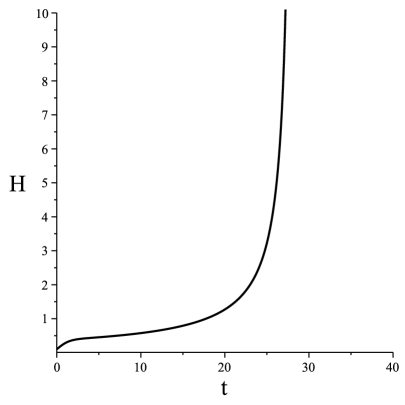
Figure 2: Stable asymptotics for $\beta=1,N=4$. The oscillations (left panel) take place for the initial values $(H_{0},\dot{H}_{0})=(0.1,0.02)$ while the runaway singularity occurs for $(H_{0},\dot{H}_{0})=(0.1,0.2)$. The ordinary matter is dust with $\gamma=1$ and $\rho_{0}=0.03$. The measure units are given in the system, where $8\pi G/3=1$, see footnote 5.

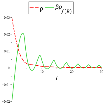
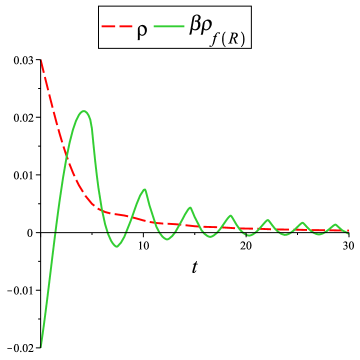
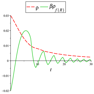
Figure 3: Matter energy density (dashed red lines) and higher-curvature corrections effective energy density (sold green lines) for an oscillatory solution depending on $\gamma$: $\gamma>\gamma_{crit}$ (upper left panel), $\gamma=\gamma_{crit}$ (upper right panel), $\gamma<\gamma_{crit}$ (bottom panel). Model parameters are $\beta=1,N=4\,({\gamma{}}_{crit}=0.8)$, initial conditions $(H_{0},\dot{H}_{0},\rho_{0})=(0.1,0.02,0.03)$; ${\gamma{}}=1.2,0.8$ and $0.3$, respectively.

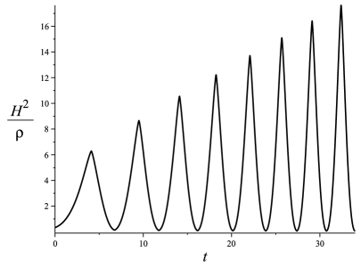
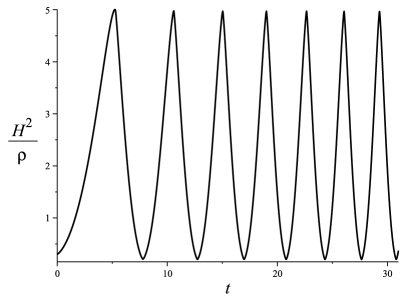
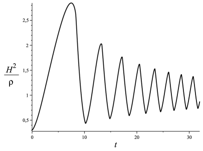
Figure 4: Fraction $H^{2}/\rho$ for oscillating solution depending on $\gamma$: $\gamma>\gamma_{crit}$ (upper left panel), $\gamma=\gamma_{crit}$ (upper right panel), $\gamma<\gamma_{crit}$ (bottom panel). Model parameters are the same with Fig.(3)

We remind the reader that for a pure $R+\beta R^{N}(N>2)$ theory the coefficient in front of the higher derivative ($f^{\prime\prime}(R)\sim|R|^{N-2}$, see (8)) may vanish for $R=0$. If this trouble occurres, then $\ddot{H}$ (or, equivalently, $\dot{R}$) diverges in order to satisfy the Eq. (8), leaving $H$ and $\dot{H}$ finite. This picture is similar to the so–called ”non-standard singularity” actively studied recently in various generalizations of GR [53, 54, 55, 56, 57, 58, 59, 60, 61, 62]. However, in most of these scenarios the Hubble derivative $\dot{H}$ diverges, keeping $H$ finite, while in our case the divergence is ”shifted” to the second derivative of the Hubble rate. Since $R$, $R_{\mu\nu}R^{\mu\nu}$ and $R_{\mu\nu\lambda\rho}R^{\mu\nu\lambda\rho}$ are expressed in terms of $H$ and $\dot{H}$ only (see, for example, [64]), then this particular situation does represent a very weak singularity with finite curvature invariants.

In the analytical part we have neglected this issue, but it is the crucial problem for a numerical procedure. However it appeared possible to remove completely this difficulty by a small change of the theory shifting minimal possible $f^{\prime\prime}(R)$ by some tiny constant into a zone of positive values. We have added the regularization term $\alpha R^{2}$ with very small coupling $\alpha\ll\beta$ which prevents the mentioned issue by making $f^{\prime\prime}=2\alpha\neq 0$ for $R=0$ and does not modify the dynamics:

$$f=R+\beta|R|^{N}\quad \to\quad f=R+\beta|R|^{N}+\alpha R^{2}:$$ (63)

$$f^{\prime\prime}=\beta N(N-1)|R|^{N-2}\quad \to\quad f^{\prime\prime}=\beta N(N-1)|R|^{N-2}+2\alpha\,.$$

In the previous section we have explored the regime where the higher-curvature term presents a small correction to the Einstein term, $\beta R^{N}\lesssim R$, i.e. the weak coupling limit. Now let us describe what happens beyond the weak coupling limit. It is well-known that in the strong coupling limit there is another type of dynamics described by the stable solution with Big Rip singularity ([27]-[33]),

$$a\propto(t_{BR}-t)^{\frac{2N^{2}-3N+1}{2-N}},\quad H\sim\frac{1}{t_{BR}-t}\,,$$

where $t_{BR}$ denotes the time of singularity.

As expected from the analysis in the Einstein frame (2) for $N>2$ we have two asymptotics: an oscillatory solution and a run-away solution. This expectation is confirmed by our numerical procedure, see Fig.2. We have obtained that low-curvature initial conditions $R_{0}(H_{0},\dot{H}_{0})\to 0$ also lead to an oscillatory solution even in the case of strong couplings $\beta\gtrsim 1$. The oscillatory solution found numerically for strong couplings exhibits the same features with that found analytically in the weak coupling limit, allowing us to identify them. Admirably, the behaviour of the energy densities of matter and HCGC depend on the interplay between the equation-of-state parameter for ordinary matter $\gamma$ and the parameter $\gamma_{crit}$, (defined by (56)) in same manner as it has been discussed in Subsec.(3.4). If ${\gamma{}}>{\gamma{}}_{crit}$ HCGC dominate over the matter contribution at late times and vice versa for ${\gamma{}}<{\gamma{}}_{crit}$, see Fig.3. In the first case the matter energy density decays with time faster than in the last case in agreement with (62). The time-behaviour of densities ratio is plotted in Fig.4 and illustrates main points of the analytical study presented in Subsec.3.4. For ${\gamma{}}<{\gamma{}}_{crit}$ the Hubble rate asymptotically tends to the GR value given by $H^{2}=\rho$ while for ${\gamma{}}<{\gamma{}}_{crit}$ we have oscillations of $H^{2}/\rho$ with an increasing amplitude.

Now let us define which initial conditions lead to each asymptotic. The basins of attraction in the initial condition space $(H_{0},\dot{H}_{0})$ for two slices of initial matter density $\rho_{0}$ are presented in Fig.5 for a set of couplings $\beta$ For numerics we have chosen one particular case of $N=4$. We clearly see that increasing the coupling $\beta$ the basin of attraction for an oscillatory solution becomes narrower (though non-vanishing) and concentrates near the parabola $R_{0}(H_{0},\dot{H}_{0})=12H^{2}_{0}+6\dot{H}_{0}=0$, while the basin of attraction for the Big-Rip solution covers more and more space.

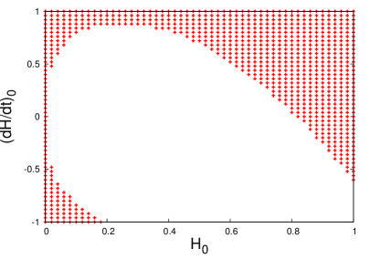
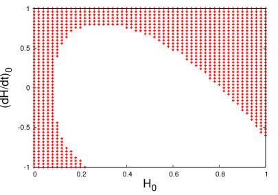
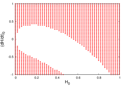
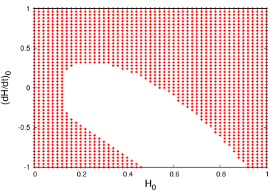
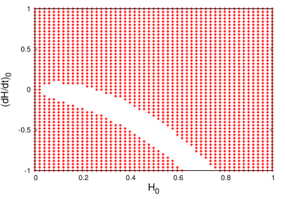
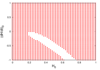
Figure 5: Basin of attraction for the Big Rip solution. $H_{0}$ and $(dH/dt)_{0}$ are initial conditions for eq. (8). Red points mark initial data, leading to the Big Rip singularity. Continuous white area corresponds to initial conditions, leading to an oscillating asymptotic. The model parameters are: $\alpha=10^{-4},N=4$, $\beta=10^{-3}$(upper panels), $\beta=10^{-2}$ (middle panels), $\beta=1$ (lower panels). On the left panels the initial density value for dust (${\gamma{}}=1$) is $\rho_{0}=0.03$; on the right panels $\rho_{0}=0.3$.

5 Conclusions

In this paper we have considered an oscillatory regime in $f(R)$ FRW cosmology with power-law functions $f=R+\beta R^{N}$. The oscillations in general appeared to be anharmonic (except the case of $N=2$) and have an effective equation of state $p_{f(R)}=(\gamma_{crit}-1)\rho_{f(R)}$ with $\gamma_{crit}=2N/(3N-2)$, meaning that for any $N>2$ these oscillations have negative effective pressure. On the other hand, $\gamma_{crit}\to 2/3$ for $N\to\infty$, being always bigger that $2/3$, so these oscillations can not cause an accelerated expansion.

The case of $N=2$ is an exceptional one in the family of power-law $f(R)$ for two further reasons: First,the coefficient at the highest derivative term in the equation of motion never vanishes in an expanding Universe. On the contrary, it may vanish for $N>2$ giving an example of a ”non-standard singularity” with finite curvature and diverging curvature time derivative. We show that such a ”singularity” (in a more general sense that the usual one, because the curvature does not diverge) is traversable and can be removed by small change in the form of $f(R)$ at least for an even $N$ (or for an arbitrary $N>1$, if we consider the theory with $f=R+\beta|R|^{N}$).

And second, there is a stable phantom-like asymptotic in the $N>2$ case which is absent for $N=2$. Initial data leading to this Big Rip regime is located in a zone of large initial curvature. If a trajectory starts from low curvature initial conditions (what value of a curvature is low enough depends on the coupling constant $\beta$ at the $R^{N}$ term) it falls into the oscillation regime.

A Generalised trigonometric functions

Everybody knows that ordinary trigonometric functions such as $\sin x$ and $\cos x$ may be defined by a trigonometric circle with the unit radius. This method is pictured on Fig. 7, where $S$ denotes an area of the shaded region. We will use similar method to define generalised sine and cosine.

Figure 6: Standard trigonometric circle with the unit radius.

Figure 7: The curve $\Gamma$ (see (66)) which has been used to define generalized trigonometric functions.

We remind the reader that the area $S$ relates to the polar angle $\varphi$ simply as $\varphi=2\,S$. Thus,

$$\cos\varphi=\cos[2\,S(\varphi)],\qquad\sin\varphi=\sin[2\,S(\varphi)].$$ (64)

Relation (64) may be expanded to the case of arbitrary $\varphi\in\mathbb{R}$: if $\varphi=\varphi_{0}+2\,\pi\,k$, where $\varphi_{0}\in[0,2\,\pi)$, $k\in\mathbb{Z}$, then $S=S_{0}+S_{\mathrm{cir}}\,k=S_{0}+\pi\,k$, where $S_{0}$ is the area of the circle, corresponding to $\varphi=\varphi_{0}$, and $S_{\mathrm{cir}}$ is the total area of the circle.

Now consider a plane curve ${\Gamma{}}$, defined by the following equation:

$${\Gamma{}}:{|x|}^{a}+{|y|}^{b}=1,$$ (65)

where $a,b>1$ (The case of $a=3/2$, $b=2$ is presented in Fig. 7). To parametrize this curve, let us go to the following generalised polar coordinates $\rho$ and $\varphi$:

$$x =\rho^{2/a}\,{|{\cos{}}\varphi|}^{2/a}\,\operatorname{sign}\cos\varphi,$$

$$y =\rho^{2/\hbox to0.0pt{$\displaystyle\scriptstyle b$\hss}\hphantom{a}}\,{|\hbox to0.0pt{$\displaystyle\displaystyle\sin$\hss}\hphantom{\cos{}}\varphi|}^{2/\hbox to0.0pt{$\displaystyle\scriptstyle b$\hss}\hphantom{a}}\,\operatorname{sign}\hbox to0.0pt{$\displaystyle\displaystyle\sin$\hss}\hphantom{\cos{}}\varphi.$$

In such coordinates the equation (65) reads as $\rho\equiv 1$, and going back to $x$ and $y$ one has:

$${\Gamma{}}:\Bigg{\{}\begin{aligned} x&={|{\cos{}}\varphi|}^{2/a}\,\operatorname{sign}\cos\varphi,\\ y&={|\hbox to0.0pt{$\displaystyle\displaystyle\sin$\hss}\hphantom{\cos{}}\varphi|}^{2/\hbox to0.0pt{$\displaystyle\scriptstyle b$\hss}\hphantom{a}}\,\operatorname{sign}\hbox to0.0pt{$\displaystyle\displaystyle\sin$\hss}\hphantom{\cos{}}\varphi.\end{aligned}$$ (66)

Further, we will consider the parameter $\varphi$ as a function of a doubled area $2S$ of the region $\Delta\Omega$, enclosed by the curve $\varphi=\mathrm{const}$, the $x$-axis and the curve $\rho=1$ (see Fig. 7):

$$\varphi=\varphi(t),\ \text{where}\ t=2\,S.$$ (67)

Note that in the Cartesian coordinates the curve $\varphi=\mathrm{const}$ may be presented in the following way (depending on the range of $\varphi$):

1. if $\cos\varphi\neq 0$,

   $$y={|x|}^{a/b}\,|\mathrm{tg}\varphi|^{2/b}\,\operatorname{sign}\sin\varphi,\quad x\in[0,\mp\infty)\quad\text{for}\,\cos\varphi\lessgtr 0;$$

2. if $\cos\varphi=0$,

   $$x=0,\quad y\in[0,\mp\infty)\quad\text{for}\,\sin\varphi\lessgtr 0.$$ (68)

Several curves of the assemblage $\varphi=\mathrm{const}$ are presented in Fig. 7. Clearly, the $\varphi$ and $S$ are in one-to-one correspondence (so $S$ and $t$ may be considered as a function of $\varphi$) and this correspondence may be expanded to arbitrary real $\varphi$ by the agreement that value

$$\varphi=\varphi_{0}+2\,\pi\,k,$$ (69)

where $\varphi_{0}\in[0,2\,\pi)$, $k\in\mathbb{Z}$, corresponds to the value

$$S=S_{0}+S_{\mathrm{cur}}\,k,$$ (69^′)

where $S_{\mathrm{cur}}$ is the area $\Omega$, enclosed by the curve ${\Gamma{}}:{|x|}^{a}+{|y|}^{b}=1$; $S_{0}$ is the area $\Delta\Omega$ of the part of $\Omega$, corresponding to the value $\varphi=\varphi_{0}$.

Next, we find a relation between $\varphi$ and $t$ by calculating the transformation Jacobian:

$$S=\iint\limits_{\Delta\Omega}dx\,dy=\iint\limits_{\Delta\omega}\Bigg{|}\frac{D(x,y)}{D(\rho,\alpha)}\Bigg{|}\,d\rho\,d\alpha,\quad\text{where}\quad\Delta\omega=\Big{\{}(\rho,\alpha)\mid\rho\in[0,1],\alpha\in[0,\varphi]\Big{\}},$$ (70)

$$\frac{D(x,y)}{D(\rho,\varphi)}=\tfrac{4}{a\,b}\,\rho^{\frac{2}{a}+\frac{2}{b}-1}\,{|{\cos{}}\varphi|}^{\frac{2}{a}-1}\,{|{\sin{}}\varphi|}^{\frac{2}{b}-1}.$$ (71)

Plugging (71) into the eq. (70) for $S$ one finds:

$$S=\tfrac{4}{a\,b}\int\limits_{0}^{1}\rho^{\frac{2}{a}+\frac{2}{b}-1}\,d\rho\int\limits_{0}^{\varphi}{|{\cos{}}\alpha|}^{\frac{2}{a}-1}\,{|{\sin{}}\alpha|}^{\frac{2}{b}-1}\,d\alpha=\\ =\tfrac{4}{a\,b}\,\tfrac{a\,b}{2\,(a+b)}\,\rho^{\frac{2\,(a+b)}{a\,b}}\Big{|}_{0}^{1}\,\int\limits_{0}^{\varphi}{|{\cos{}}\alpha|}^{\frac{2}{a}-1}\,{|{\sin{}}\alpha|}^{\frac{2}{b}-1}\,d\alpha=\tfrac{2}{a+b}\int\limits_{0}^{\varphi}{|{\cos{}}\alpha|}^{\frac{2}{a}-1}\,{|{\sin{}}\alpha|}^{\frac{2}{b}-1}\,d\alpha.$$ (72)

Using $t=2\,S$, we obtain the final relation between $t$ and $\varphi$:

$$t=\tfrac{4}{a+b}\int\limits_{0}^{\varphi}{|{\cos{}}\alpha|}^{\frac{2}{a}-1}\,{|{\sin{}}\alpha|}^{\frac{2}{b}-1}\,d\alpha.$$ (73)

The relation (73) (for fixed $a$ and $b$) defines one-to-one correspondence between $t$ and $\varphi$. Let us denote its solution with respect to $\varphi$ as $\varphi(a,b;t)$. Clearly, $\varphi(a,b;t)$ may not be expressed in elementary functions for arbitrary values of $a$ and $b$. Using the function $\varphi(a,b;t)$, let us introduce sine and cosine of order ${\bf p}=\{a,b\}$.

Definition 1

Functions

$$\operatorname{Cos}(a,b;t) ={|{\cos{}}\varphi(a,b;t)|}^{2/a}\,\operatorname{sign}\cos\varphi(a,b;t),$$ (74)

$$\@ADDCLASS{ltx_eqn_lefteqn}$\displaystyle\displaystyle\operatorname{Sin}$\mbox{}\hfil\hphantom{\operatorname{Cos}}(a,b;t) ={|\hbox to0.0pt{$\displaystyle\displaystyle\sin$\hss}\hphantom{\cos{}}\varphi(a,b;t)|}^{2/\hbox to0.0pt{$\displaystyle\scriptstyle b$\hss}\hphantom{a}}\,\operatorname{sign}\hbox to0.0pt{$\displaystyle\displaystyle\sin$\hss}\hphantom{\cos{}}\varphi(a,b;t)$$

are called the cosine and the sine of order p $=\{a,b\}$ respectively.

We will omit $a$ and $b$ in the places, where we use a sine and a cosine of the same order, i.e. to write $\operatorname{Cos}t$, $\operatorname{Sin}t$ and $\varphi(t)$ instead of $\operatorname{Cos}(a,b;t)$, $\operatorname{Sin}(a,b;t)$ and $\varphi(a,b;t)$. Moreover, we will call the functions $\operatorname{Cos}t$ and $\operatorname{Sin}t$ just as generalized cosine and sine. As it may be seen from (74) and (66), functions $\operatorname{Cos}t$ and $\operatorname{Sin}t$ represent correspondingly coordinates $x$ and $y$ of a crossing point of the curves ${\Gamma{}}$ and $\varphi=\mathrm{const}$, enclosing the area $S=t/2$ (see Fig. 7).

Let us find differential equations for $\operatorname{Cos}(a,b;t)$ and $\operatorname{Sin}(a,b;t)$. From the definition (74) we have (a prime denotes derivative with respect to $t$)

$${(\operatorname{Cos}t)}^{\prime} ={}-\tfrac{2}{a}\,{|{\cos{}}\varphi(t)|}^{\frac{2}{a}-1}\,[\hbox to0.0pt{$\displaystyle\displaystyle\sin$\hss}\hphantom{\cos{}}\varphi(t)]\,\varphi^{\prime}(t),$$ (75)

$${(\hbox to0.0pt{$\displaystyle\displaystyle\operatorname{Sin}$\hss}\hphantom{\operatorname{Cos}{}}t)}^{\prime} =\hbox to0.0pt{$\displaystyle\displaystyle{}+{}$\hss}\hphantom{{}-{}}\tfrac{2}{\hbox to0.0pt{$\displaystyle\scriptstyle b$\hss}\hphantom{a}}\,{|\hbox to0.0pt{$\displaystyle\displaystyle\sin$\hss}\hphantom{\cos{}}\varphi(t)|}^{\frac{2}{\hbox to0.0pt{$\displaystyle\scriptscriptstyle b$\hss}\hphantom{a}}-1}\,[\cos\varphi(t)]\,\varphi^{\prime}(t).$$

The derivative $\varphi^{\prime}(t)$ may be expressed from (73):

$$\varphi^{\prime}(t)=\tfrac{a+b}{4}\,{|{\cos{}}\varphi(t)|}^{1-\frac{2}{a}}\,{|{\sin{}}\varphi(t)|}^{1-\frac{2}{b}}.$$ (76)

Plugging (76) into (75), we have

$${(\operatorname{Cos}t)}^{\prime} ={}-\tfrac{a+b}{2\,a}\,{|\hbox to0.0pt{$\displaystyle\displaystyle\sin$\hss}\hphantom{\cos{}}\varphi(t)|}^{\frac{2}{\hbox to0.0pt{$\displaystyle\scriptscriptstyle b$\hss}\hphantom{a}}(\hbox to0.0pt{$\displaystyle\scriptstyle b$\hss}\hphantom{a}-1)}\,\operatorname{sign}\hbox to0.0pt{$\displaystyle\displaystyle\sin$\hss}\hphantom{\cos{}}\varphi(t)={}-\tfrac{a+b}{2\,a}\,{|\hbox to0.0pt{$\displaystyle\displaystyle\operatorname{Sin}$\hss}\hphantom{\operatorname{Cos}{}}t|}^{\hbox to0.0pt{$\displaystyle\scriptstyle b$\hss}\hphantom{a}-1}\,\operatorname{sign}\hbox to0.0pt{$\displaystyle\displaystyle\operatorname{Sin}$\hss}\hphantom{\operatorname{Cos}{}}t,$$ (77)

$${(\hbox to0.0pt{$\displaystyle\displaystyle\operatorname{Sin}$\hss}\hphantom{\operatorname{Cos}{}}t)}^{\prime} =\hbox to0.0pt{$\displaystyle\displaystyle{}+{}$\hss}\hphantom{{}-{}}\tfrac{a+b}{2\,b}\,{|{\cos{}}\varphi(t)|}^{\frac{2}{a}(a-1)}\,\operatorname{sign}\cos\varphi(t)=\hbox to0.0pt{$\displaystyle\displaystyle{}+{}$\hss}\hphantom{{}-{}}\tfrac{a+b}{2\,b}\,{|{\operatorname{Cos}{}}t|}^{a-1}\,\operatorname{sign}\operatorname{Cos}t.$$ (78)

Using the identity (see. (74), (65)):

$${|{\operatorname{Cos}{}}t|}^{a}+{|{\operatorname{Sin}{}}t|}^{b}\equiv 1,$$ (79)

we obtain

$${|\hbox to0.0pt{$\displaystyle\displaystyle\operatorname{Sin}$\hss}\hphantom{\operatorname{Cos}{}}t|}^{\hbox to0.0pt{$\displaystyle\scriptstyle b$\hss}\hphantom{a}-1} \equiv{\big{(}1-{|{\operatorname{Cos}{}}t|}^{a}\big{)}}^{\frac{\hbox to0.0pt{$\displaystyle\scriptscriptstyle b$\hss}\hphantom{a}-1}{b}},$$ (80)

$${|{\operatorname{Cos}{}}t|}^{a-1} \equiv{\big{(}1-{|\hbox to0.0pt{$\displaystyle\displaystyle\operatorname{Sin}$\hss}\hphantom{\operatorname{Cos}{}}t|}^{\hbox to0.0pt{$\displaystyle\scriptstyle b$\hss}\hphantom{a}}\big{)}}^{\frac{a-1}{a}}.$$ (81)

Clearly, from (77) and (80) one has

$${\big{(}\tfrac{2\,a}{a+b}\big{)}}^{\frac{b}{b-1}}\,{|{\operatorname{Cos}^{\prime}t}|}^{\frac{b}{b-1}}+{|{\operatorname{Cos}t}|}^{a}=1.$$

Using the fact that $\operatorname{Cos}0=1$ (see (74) and (73)), we conclude that the function $z=\operatorname{Cos}t$ is a solution of the following Cauchi problem:

$${\big{(}\tfrac{2\,a}{a+b}\big{)}}^{\frac{b}{b-1}}\,{|\dot{z}|}^{\frac{b}{b-1}}+{|z|}^{a}=1,$$ (82a)

$$z(0)=1.$$ (82b)

Perming similar actions, using (78), (81) and the fact that $\operatorname{Sin}0=0$ (see (74), (73)), we obtain the following initial problem for the function $z=\operatorname{Sin}t$:

$${\big{(}\tfrac{2\,b}{a+b}\big{)}}^{\frac{a}{a-1}}\,{|\dot{z}|}^{\frac{a}{a-1}}+{|z|}^{b}=1,$$ (83a)

$$z(0)=0.$$ (83b)

Equation (82a) for $\operatorname{Cos}t$ is not resolved with respect to a higher derivative. To get such kind of equation, let us take one more derivative of (82a):

$${\big{(}\tfrac{2\,a}{a+b}\big{)}}^{\frac{b}{b-1}}\,\tfrac{b}{b-1}\,{|\dot{z}|}^{\frac{1}{b-1}}\,(\operatorname{sign}\dot{z})\,\ddot{z}+a\,{|z|}^{a-1}\,(\operatorname{sign}z)\,\dot{z}=0.$$ (84)

Using eq. (82b), $\operatorname{Cos}^{\prime}0=0$ (see. (75) and (73)), we get the following second-order Cauchi problem for $z=\operatorname{Cos}t$:

$$\tfrac{b}{b-1}\,{\big{(}\tfrac{2\,a}{a+b}\big{)}}^{\frac{b}{b-1}}\,{|\dot{z}|}^{\frac{2-b}{b-1}}\,\ddot{z}+a\,{|z|}^{a-2}\,z=0,$$

$$z(0)=1,\quad\dot{z}(0)=0.$$

Similarly, from (83a), (83b), $\operatorname{Sin}^{\prime}0=(a+b)/(2\,b)$ (see. (75), (73) and  (76)), we find the initial problem for $z=\operatorname{Sin}t$:

$$\tfrac{a}{a-1}\,{\big{(}\tfrac{2\,b}{a+b}\big{)}}^{\frac{a}{a-1}}\,{|\dot{z}|}^{\frac{2-a}{a-1}}\,\ddot{z}+b\,{|z|}^{b-2}\,z=0,$$ (85)

$$z(0)=0,\quad\dot{z}(0)=\tfrac{a+b}{2\,b}.$$ (86)

Next, let us study some useful features of $\operatorname{Cos}t$ and $\operatorname{Sin}t$. First of all, from the initial geometrical interpretation (see Fig. 7) one concludes that $\operatorname{Cos}t$ and $\operatorname{Sin}t$ are periodic functions with the period $T=2\,S_{\mathrm{cur}}$, where $S_{\mathrm{cur}}$ is the square of area $\Omega$, enclosed by the curve ${\Gamma{}}$:

$$\operatorname{Cos}(a,b;t+T)\equiv\operatorname{Cos}(a,b;t),\qquad\operatorname{Sin}(a,b;t+T)\equiv\operatorname{Sin}(a,b;t).$$ (87)

To find $T$ one should use the fact that the expression (72) for area $\Delta\Omega$ in between the curve $\varphi=\mathrm{const}$ and $X$-axis coincides with the $\Omega$ for $\varphi=2\,\pi$:

$$T=2\,S_{\mathrm{cur}}=\tfrac{4}{a+b}\,\int\limits_{0}^{2\,\pi}{|{\cos{}}\alpha|}^{\frac{2}{a}-1}\,{|{\sin{}}\alpha|}^{\frac{2}{b}-1}\,d\alpha.$$ (88)

The period $T$ may be expressed in terms of the Euler’s Gamma ${\Gamma{}}(x)$ and Beta $B(x,y)$ functions. From (88) one writes

$$\int\limits_{0}^{2\,\pi}{|{\cos{}}\alpha|}^{\frac{2}{a}-1}\,{|{\sin{}}\alpha|}^{\frac{2}{b}-1}\,d\alpha=4\,\int\limits_{0}^{\pi/2}{\big{(}{\cos^{2}{}}\alpha\big{)}}^{\frac{1}{a}-1}\,{\big{(}{\sin^{2}{}}\alpha\big{)}}^{\frac{1}{b}-1}\,\cos\alpha\,\sin\alpha\,d\alpha=\\ =\int\limits_{\pi/2}^{0}{\big{(}\tfrac{1+\cos 2\alpha}{2}\big{)}}^{\frac{1}{a}-1}\,{\big{(}\tfrac{1-\cos 2\alpha}{2}\big{)}}^{\frac{1}{b}-1}\,d\cos 2\alpha=\int\limits_{-1}^{+1}{\big{(}\tfrac{1+u}{2}\big{)}}^{\frac{1}{a}-1}\,{\big{(}\tfrac{1-u}{2}\big{)}}^{\frac{1}{b}-1}\,du.$$

Using (88) and performing the change of variable $u=2\,v-1$, we get the final result:

$$T=\tfrac{8}{a+b}\,\int\limits_{0}^{1}\,v^{\frac{1}{a}-1}\,{(1-v)}^{\frac{1}{b}-1}\,dv=\tfrac{8}{a+b}\,B(\tfrac{1}{a},\tfrac{1}{b})=\tfrac{8}{a+b}\,\tfrac{{\Gamma{}}(\frac{1}{a})\,{\Gamma{}}(\frac{1}{b})}{{\Gamma{}}(\frac{1}{a}+\frac{1}{b})}.$$ (89)

For $a=b=2$ the period $T$ reduces to well-known value

$$T=2\,\tfrac{{\Gamma{}}(1/2)\,{\Gamma{}}(1/2)}{{\Gamma{}}(1)}=2\,\tfrac{\sqrt{\pi}\,\sqrt{\pi}}{1}=2\,\pi,$$

as expected from the fact that $\operatorname{Cos}t$ and  $\operatorname{Sin}t$ of order ${\bf p}=\{2,2\}$ are ordinary trigonometric functions (see (74) and (73)):

$$\operatorname{Cos}(2,2;t)=\cos t,\qquad\operatorname{Sin}(2,2;t)=\sin t.$$

Finally, from the Def. 1 and $\varphi(-t)=-\varphi(t)$ (as a consequence of (69), (69^′) and our agreement to expand $\varphi$ and $S=2\,t$ to all real numbers) we obtain evenness of $\operatorname{Cos}t$ and oddness of $\operatorname{Sin}t$:

$$\operatorname{Cos}(-t)=\operatorname{Cos}t,\qquad\operatorname{Sin}(-t)={}-\operatorname{Sin}t.$$

Now we are equipped to solve the eq.(21). Performing the change of variable

$$\tilde{\psi}=\tfrac{4(N-1)}{3N-2}(C_{1}^{2}-C_{2})^{\frac{2-N}{2N}}\tau+\text{const}\,,$$ (90)

our equation transforms to:

$$\nu^{N}|z^{\prime}|^{N}+z^{2}=1\,,\quad\text{where}\quad z\equiv\frac{H-C_{1}}{\sqrt{C_{1}^{2}-C_{2}}}\,,\quad z^{\prime}=\frac{dz}{d\tilde{\psi}}\,,\quad\frac{4(N-1)}{3N-2}\equiv\nu\,.$$ (91)

Comparing this with (83a) one finds solutions of the eqs.(21),(15b):

$$H =C_{1}+\sqrt{C_{1}^{2}-C_{2}}\;\text{Sin}(\tfrac{N}{N-1},2;\tilde{\psi})\,,\quad\text{where}\quad\tilde{\psi}=\nu(C_{1}^{2}-C_{2})^{\tfrac{2-N}{2N}}\tau+\text{const}\,,$$ (92)

$$Q=H_{\tau} =\nu\sqrt[N]{C_{1}^{2}-C_{2}}\;\text{Sin}^{\prime}(\tfrac{N}{N-1},2;\tilde{\psi})\,=$$

$$=\sqrt[N]{C_{1}^{2}-C_{2}}\;\sqrt[N]{1-\operatorname{Sin}^{2}(\tfrac{N}{N-1},2;\tilde{\psi})}\,\operatorname{sign}\operatorname{Sin}^{\prime}(\tfrac{N}{N-1},2;\tilde{\psi})\,.$$ (93)

Introducing new notations and absorbing constant $\nu$ in the independent variable $\tilde{\psi}$ we get:

$$\text{Sin}({\displaystyle{\tiny\tfrac{N}{N-1}}},2;\tilde{\psi}) \equiv\sin_{N}(\psi)\,,\quad\text{where}\quad\psi\equiv(C_{1}^{2}-C_{2})^{\frac{2-N}{2N}}\tau+\text{const}\,,$$ (94)

$$\text{Cos}({\displaystyle{\tiny\tfrac{N}{N-1}}},2;\tilde{\psi}) \equiv\cos_{N}(\psi)\,,$$ (95)

$$\operatorname{sign}\operatorname{Sin}^{\prime}(\tfrac{N}{N-1},2;\tilde{\psi}) =\operatorname{sign}Q(\tau)\equiv\operatorname{Sg}_{N}(\psi)\,,$$ (96)

$$\frac{\partial}{\partial\psi}\sin_{N}(\psi) =\operatorname{Sg}_{N}(\psi)\sqrt[N]{1-\sin_{N}^{2}(\psi)}\,;$$ (97)

and write down final solution of an unperturbed system:

$$H =H(C_{1},C_{2},\psi)\equiv C_{1}+\sqrt{C_{1}^{2}-C_{2}}\sin_{N}(\psi)\,,$$ (98a)

$$Q =Q(C_{1},C_{2},\psi)\equiv\operatorname{Sg}_{N}(\psi)\sqrt[N]{C_{1}^{2}-C_{2}}\sqrt[N]{1-\sin^{2}_{N}(\psi)}\,,$$ (98b)

$$\rho =\rho(C_{1},C_{2},\psi)\equiv C_{2}\,.$$ (98c)

Finally, since $\tilde{\psi}=\nu\psi$ (see (92),(94)), the period $T_{0}$ of the function $\sin_{N}(\psi)$ is $\nu$ times smaller than the period $T$ of the function $\operatorname{Sin}(\tfrac{N}{N-1},2;\tilde{\psi})$:

$$T_{0}=\tfrac{1}{\nu}T=2B(\tfrac{1}{2},\tfrac{N-1}{N})\,.$$ (99)

References

[1]
T. Clifton; P. G. Ferreira; A. Padilla; C. Skordis,
”Modified Gravity and Cosmology,”
[arXiv:1106.2476].
[2] S. Perlmutter et al., Astrophys. J. 517, 565 (1999).
[3] A.G. Riess et al., Astron. J. 116, 1009 (1998).
[4]
A. Starobinsky,
JETP Lett., 86, 157-163, (2007)
[arXiv:0706.2041].
[5]
W. Hu, I. Sawicky,
Phys. Rev. D 76 , 064004 (2007)
[arXiv:0705.1158].
[6]
J-Q. Guo, A.V. Frolov,
”Cosmological evolution in f(R) gravity and a logarithmic model,”
[arXiv:1305.7290].
[7]
T. Sotiriou,
”Modified Actions for Gravity: Theory and Phenomenology,”
[arXiv:0710.4438].
[8]
A. De Felice, S. Tsujikawa,
Living Reviews in Relativity, 3, vol. 13. (2010)
[arXiv:1002.4928].
[9]
T. P. Sotiriou, V. Faraoni,
Rev. Mod. Phys. 82, 451-497 (2010).
[arXiv:0805.1726].
[10]
T. P. Sotiriou,
J.Phys.Conf.Ser.189:012039 (2009) [arXiv:0810.5594].
[11]
S. Nojiri, S. Odintsov,
eConf C0602061 (2006) 06,
Int.J.Geom.Meth.Mod.Phys. 4 (2007) 115-146, [arXiv:hep-th/0601213].
[12]
S. Nojiri, S. Odintsov,
Phys.Rept. 505 (2011) 59-144, [arXiv:1011.0544].
[13]
R. R. Caldwell, M. Kamionkowski and N. N. Weinberg,
Phys. Rev. Lett. 91, 071301 (2003)
[arXiv:astro-ph/0302506].
[14]
M. Carroll, M. Hoffman and M. Trodden, Phys. Rev.
D 68, 023509 (2003) [arXiv:astro-ph/0301273].
[15]
S. Nojiri and S. D. Odintsov,
Phys. Lett. B 562, 147 (2003) [arXiv:hep-th/0303117]; Phys. Lett. B 565,
1 (2003) [arXiv:hep-th/0304131].
[16]
E. Elizalde, S. Nojiri and S. D. Odintsov,
Phys. Rev. D 70, 043539 (2004) [arXiv:hep-th/0405034].
[17]
M. Sami and A. Toporensky, Mod. Phys. Lett. A 19, 1509
(2004) [arXiv:gr-qc/0312009].
[18]
S. Tsujikawa, Class. Quant. Grav. 20, 1991 (2003)
[arXiv:hep-th/0302181].
[19]
F. Piazza and S. Tsujikawa, JCAP 0407, 004 (2004) [arXiv:hep-th/0405054].
[20]
A. Vikman, Phys.Rev. D71 023515, (2005) [arXiv:astro-ph/0407107].
[21]
S. M. Carroll, A. De Felice and M. Trodden, Phys. Rev. D71, 023525 (2005) [arXiv:astro-ph/0408081].
[22]
S. Tsujikawa and M. Sami, Phys. Lett. B 603, 113 (2004) [arXiv:hep-th/0409212].
[23]
S. Nojiri and S. D. Odintsov, PoS WC2004 (2004) 024, [arXiv:hep-th/0412030];
[24]
B. Gumjudpai, T. Naskar, M. Sami and S. Tsujikawa, JCAP 0506:007 (2005) [arXiv:hep-th/0502191];
[25]
H. Stefancic, Phys.Rev. D71 124036, (2005). [arXiv: astro-ph/0504518];
[26]
A. A. Andrianov, F. Cannata and A. Y. Kamenshchik, Phys.Rev.D72:043531, (2005) [arXiv:gr-qc/0505087].
[27]
S. Capozziello, F. Occhionero and
L. Amendola,
IJMPD 1, 615 (1992).
[28]
V. Muller, H.-J. Schmidt and A. A. Starobinsky,
Phys. Lett. B 202, 198 (1988).
[29]
H.-J. Schmidt,
Class. Quant. Grav. 6, 557 (1989),
V. Muller, H.-J. Schmidt and A. A. Starobinsky,
Class. Quant.
Grav. 7, 1163 (1990).
[30] S. Carloni, K. S. Dunsby, S. Capozziello, A. Troisi, Class. Quant. Grav., 22, 4839 (2005)
[arXiv:gr-qc/0410046].
[31] S. Carloni, A. Troisi, P. K. S. Dunsby,
Gen. Rel. Grav.,41, 1757 (2009). 083504(2007)
[arXiv:0706.0452].
[32]
M. M. Ivanov, A. V. Toporensky, IJMPD, 21, 1250051
(2012) [arXiv:1112.4194].
[33]
M. M. Ivanov, A. V. Toporensky, Grav.Cosmol. 18, 43-53 (2012)
[arXiv:1106.5179].
[34]
A. Starobinsky, Phys.
Lett.B 91: 99-102, (1980).
[35]
J. Miritzis,
Gen.Rel.Grav. 41:49-65, (2009) [arXiv:0708.1396].