Decoherence effects in the quantum qubit flip game using Markovian approximation

Abstract

We are considering a quantum version of the penny flip game, whose implementation is influenced by the environment that causes decoherence of the system. In order to model the decoherence we assume Markovian approximation of open quantum system dynamics. We focus our attention on the phase damping, amplitude damping and amplitude raising channels. Our results show that the Pauli strategy is no longer a Nash equilibrium under decoherence. We attempt to optimize the players’ control pulses in the aforementioned setup to allow them to achieve higher probability of winning the game compared to the Pauli strategy.

1 Introduction

Quantum information experiments can be described as a sequence of three operations: state preparation, evolution and measurement [5]. In most cases one cannot assume that experiments are conducted perfectly, therefore imperfections have to be taken into account while modelling them. In this work we are interested in how the knowledge about imperfect evolution of a quantum system can be exploited by players engaged in a quantum game. We assume that one of the players possesses the knowledge about imperfections in the system, while the other is ignorant of their existence. We ask a question of how much the player’s knowledge about those imperfections can be exploited by him/her for their advantage.

We consider implementation of the quantum version of the penny flip game, which is influenced by the environment that causes decoherence of the system. In order to model the decoherence we assume Markovian approximation of open quantum system dynamics.

The paper is organised as follows: in the two following subsections we discuss related work and present our motivation to undertake this task. In Section 2 we recall the penny flip game and its quantum version, in Section 3 we present the noise model, in Section 4 we discuss the strategies applied in the presence of noise and finally in Section 5 we conclude the obtained results.

1.1 Related work

Imperfect realizations of quantum games have been discussed in literature since the beginning of the century. Ref. [7] discusses a three-player quantum game played with a corrupted source of entangled qubits. The author implicitly assumes that the initial state of the game had passed through a bit-flip noisy channel before the game began. The corruption of quantum states in schemes implementing quantum games was studied by various authors i.e. in [1] the authors perform an analysis of the two-player prisoners dilemma game, in [2] the multiplayer quantum minority game with decoherence is studied, in [4, 13] the authors analyse the influence of the local noisy channels on quantum Magic Squares games, while the quantum Monty Hall problem under decoherence is studied first in [3] and subsequently in [8]. In [9] the authors study the influence of the interaction of qubits forming a spin chain on the qubit flip game. An analysis of trembling hand perfect equilibria in quantum games was done in [12]. Prisoners’ dilemma in the presence of collective dephasing modelled by using the Markovian approximation of open quantum systems dynamics is studied in [10]. Unfortunately the model applied in this work assumes that decoherence acts only after the initial state has been prepared and ceases to act before unitary strategies are applied.

1.2 Motivation

In the quantum game theoretic literature decoherence is typically applied to a quantum game in the following way:

1. the entangled state is prepared,

2. it is transferred through a local noisy channel,

3. players’ strategies are applied,

4. the resulting state is transferred once again through a local noisy channel,

5. the state is disentangled,

6. quantum local measurements are performed and the outcomes of the games are calculated.

In some cases, where it is appropriate, steps 4 and 5 are omitted. The problem with the above procedure is that it separates unitary evolution from the decoherent evolution. In [9] it was proposed to observe the behaviour of the quantum version of the penny flip game under more physically realistic assumptions where decoherence due to coupling with the environment and unitary evolution happen simultaneously.

2 Game as a quantum experiment

In this work our goal is to follow the work done in [9] and to discuss the quantum penny flip game as a physical experiment consisting in preparation, evolution and measurement of the system. For the purpose of this paper we assume that preparation and measurement, contrary to noisy evolution of the system are perfect. We investigate the influence of the noise on the players’ odds and how the noisiness of the system can be exploited by them. The noise model we use is described by the Lindblad master equation and the dynamics of the system is expressed in the language of quantum systems control.

2.1 Penny flip game

In order to provide classical background for our problem, let us consider a classical two-player game, consisting in flipping over a coin by the players in three consecutive rounds. As usual, the players are called Alice and Bob. In each round Alice and Bob performs one of two operations on the coin: flips it over or retains it unchanged.

At the beginning of the game, the coin is turned heads up. During the course of the game the coin is hidden and the players do not know the opponents actions. If after the last round the coin is tails up, then Alice wins, otherwise the winner is Bob.

The game consists of three rounds: Alice performs her action in the first and the third round, while Bob performs his in the second round of the game. Therefore the set of allowed strategies consists of eight sequences $(N,N,N),(N,N,F),$ $\ldots,(F,F,F)$, where $N$ corresponds to the non-flipping strategy and $F$ to the flipping strategy. Bob’s pay-off table for this game is presented in Table 1. Looking at the pay-off tables, it can be seen that utility function of players in the game is balanced, thus the penny flip game is a zero-sum game.

	$NN$	$FN$	$NF$	$FF$
$N$	$1$	$-1$	$-1$	$1$
$F$	$-1$	$1$	$1$	$-1$

Table 1: Bob’s pay-off table for the penny flip game.

A detailed analysis of this game and its asymmetrical quantization can be found in [14]. In this work it was shown that there is no winning strategy for any player in the penny flip game. It was also shown, that if Alice was allowed to extend her set of strategies to quantum strategies she could always win. In [9] it was shown that when both players have access to quantum strategies the game becomes fair and it has the Nash equilibrium.

2.2 Qubit flip game

Following the work done in the aforementioned paper [9] we consider a quantum version of the penny flip game. In this case, we treat a qubit as a quantum coin. As in the classical case the game is divided into three rounds. Starting with Alice, in each round, one player performs a unitary operation on the quantum coin. The rules of the game are constrained by its physical implementation. We assume that in each round each of the players can choose three control parameters $\alpha_{1},\alpha_{2},\alpha_{3}$ in order to realise his/her strategy. The resulting unitary gate is given by the equation:

$$U(\alpha_{1},\alpha_{2},\alpha_{3})=e^{-\mathrm{i}\alpha_{3}\sigma_{z}\Delta t}e^{-\mathrm{i}\alpha_{2}\sigma_{y}\Delta t}e^{-\mathrm{i}\alpha_{1}\sigma_{z}\Delta t},$$ (1)

where $\Delta t$ is an arbitrarily chosen constant time interval.

Therefore, the system defined above forms a single qubit system driven by time-dependent Hamiltonian $H(t)$, which is a piecewise constant and can be expressed in the following form

$$H(t)=\begin{cases}\alpha_{1}^{A_{1}}\sigma_{z}&\text{ for }0\leq t<\Delta t,\\ \alpha_{2}^{A_{1}}\sigma_{y}&\text{ for }\Delta t\leq t<2\Delta t,\\ \alpha_{3}^{A_{1}}\sigma_{z}&\text{ for }2\Delta t\leq t<3\Delta t,\\ \alpha_{1}^{B}\sigma_{z}&\text{ for }3\Delta t\leq t<4\Delta t,\\ \alpha_{2}^{B}\sigma_{y}&\text{ for }4\Delta t\leq t<5\Delta t,\\ \alpha_{3}^{B}\sigma_{z}&\text{ for }5\Delta t\leq t<6\Delta t,\\ \alpha_{1}^{A_{2}}\sigma_{z}&\text{ for }6\Delta t\leq t<7\Delta t,\\ \alpha_{2}^{A_{2}}\sigma_{y}&\text{ for }7\Delta t\leq t<8\Delta t,\\ \alpha_{3}^{A_{2}}\sigma_{z}&\text{ for }8\Delta t\leq t\leq 9\Delta t.\end{cases}$$ (2)

Control parameters in the Hamiltonian $H(t)$ will be referred to vector $\mathrm{\alpha}=(\alpha_{1}^{A_{1}},\alpha_{1}^{A_{1}},\alpha_{2}^{A_{1}},\alpha_{2}^{A_{1}},\alpha_{1}^{B},\alpha_{2}^{B},\alpha_{3}^{B},\alpha_{1}^{A_{2}},\alpha_{2}^{A_{2}},\alpha_{3}^{A_{2}})$, where $\alpha_{i}^{A_{j}}$ are determined by Alice and $\alpha_{i}^{B}$ are selected by Bob.

Suppose that players are allowed to play the game by manipulating the control parameters in the Hamiltonian $H(t)$ representing the coherent part of the dynamics, but they are not aware of the action of the environment on the system. Hence the time evolution of the system is non-unitary and is described by a master equation, which can be written generally in the Lindblad form as

$$\frac{\mathrm{d}\rho}{\mathrm{d}t}=-\mathrm{i}[H(t),\rho]+\sum_{j}\gamma_{j}(L_{j}\rho L_{j}^{\dagger}-\frac{1}{2}\{L_{j}^{\dagger}L_{j},\rho\}),$$ (3)

where $H(t)$ is the system Hamiltonian, $L_{j}$ are the Lindblad operators, representing the environment influence on the system [11] and $\rho$ is the state of the system.

For the purpose of this paper we chose three classes of decoherence: amplitude damping, amplitude raising and phase damping which correspond to noisy operators $\sigma_{-}=|0\rangle\langle 1|$, $\sigma_{+}=|1\rangle\langle 0|$ and $\sigma_{z}$, respectively.

Let us suppose that initially the quantum coin is in the state $|0\rangle\langle 0|$. Next, in each round, Alice and Bob perform their sequences of controls on the qubit, where each control pulse is applied according to equation (3). After applying all of the nine pulses, we measure the expected value of the $\sigma_{z}$ operator. If $\mathrm{tr}(\sigma_{z}\rho(T))=-1$ Alice wins, if $\mathrm{tr}(\sigma_{z}\rho(T))=1$ Bob wins. Here, $\rho(T)$ denotes the state of the system at time $T=9\Delta t$.

Alternatively we can say that the final step of the procedures consists in performing orthogonal measurement$\{O_{\rm heads}\to|0\rangle\langle 0|,O_{\rm tails}\to|1\rangle\langle 1|\}$ on state $\rho(T)$. The probability of measuring $O_{\rm heads}$ and $O_{\rm tails}$ determines pay-off functions for Alice and Bob, respectively. These probabilities can be obtained from relations $p(\mathrm{heads})=\langle 1|\rho(T)|1\rangle$ and $p(\mathrm{tails})=\langle 0|\rho(T)|0\rangle$.

2.3 Nash equilibrium

In this game, pure strategies cannot be in Nash equilibrium. Hence, the players choose mixed strategies, which are better than the pure ones. We assume that Alice and Bob use the Pauli strategy, which is mixed and gives Nash equilibrium [9], therefore this strategy is a reasonable choice for the players. According to the Pauli strategy, each player chooses one of the four unitary operations $\{\mathbb{1},\mathrm{i}\sigma_{x},\mathrm{i}\sigma_{y},\mathrm{i}\sigma_{z}\}$ with equal probability. Thus, to obtain the Pauli strategy, each player chooses a sequence of control parameters $(\xi_{1},\xi_{1},\xi_{2})$ listed in Tab. 2. It means that in each round, one player performs a unitary operation chosen randomly with a uniform probability distribution from the set $\{\mathbb{1},\mathrm{i}\sigma_{x},\mathrm{i}\sigma_{y},\mathrm{i}\sigma_{z}\}$.

	$\xi_{1}$	$\xi_{2}$	$\xi_{3}$
$\mathbb{1}$	$0$	$0$	$0$
$\mathrm{i}\sigma_{x}$	$\frac{\pi}{4}$	$-\frac{\pi}{2}$	$-\frac{\pi}{4}$
$\mathrm{i}\sigma_{y}$	$0$	$-\frac{\pi}{2}$	$0$
$\mathrm{i}\sigma_{z}$	$-\frac{\pi}{4}$	$0$	$-\frac{\pi}{4}$

Table 2: Control parameters for realising the Pauli strategy. The left column indicates the resulting gate.

3 Influence of decoherence on the game

In this section, we perform an analytical investigation which shows the influence of decoherence on the game result. In accordance with the Lindblad master equation, the environment influence on the system is represented by Lindblad operators $L_{j}$, while the rate of decoherence is described by parameters $\gamma_{j}$. To simplify the discussion, we consider Hamiltonians $H(t)$ represented by diagonal matrices, i.e. in the following form $H(t)=\beta_{1}|0\rangle\langle 0|+\beta_{2}|1\rangle\langle 1|$.

3.1 Amplitude damping and amplitude raising

First we consider the amplitude damping decoherence, which corresponds to the Lindblad operator $\sigma_{-}$. Thus the master equation (3) is expressed as

$$\frac{\mathrm{d}\rho}{\mathrm{d}t}=-\mathrm{i}[H(t),\rho]+\gamma(\sigma_{-}\rho\sigma_{+}-\frac{1}{2}\sigma_{+}\sigma_{-}\rho-\frac{1}{2}\ \rho\sigma_{+}\sigma_{-}),$$ (4)

where $\sigma_{+}=\sigma_{-}^{\dagger}=|1\rangle\langle 0|$. The equation can be rewritten in the following form

$$\frac{\mathrm{d}\rho}{\mathrm{d}t}=A\rho+\rho A^{\dagger}+\gamma\sigma_{-}\rho\sigma_{+},$$ (5)

where $A=-\mathrm{i}H(t)-\frac{1}{2}\gamma\sigma_{+}\sigma_{-}$. In solving this equation it is helpful to make a change of variables $\rho(t)=e^{At}\hat{\rho}(t)e^{A^{\dagger}t}$. Hence, we obtain

$$\frac{\mathrm{d}\hat{\rho}}{\mathrm{d}t}=\gamma B(t)\hat{\rho}(t)B^{\dagger}(t),$$ (6)

where $B(t)=e^{-At}\sigma_{-}e^{At}=e^{-\mathrm{i}(\beta_{2}-\beta_{1})t-\frac{\gamma}{2}t}\sigma_{-}$. It follows that

$$\frac{\mathrm{d}\hat{\rho}}{\mathrm{d}t}=\gamma e^{-\gamma t}\sigma_{-}\hat{\rho}(t)\sigma_{+}.$$ (7)

Due to the fact that $\sigma_{-}\sigma_{-}=\sigma_{+}\sigma_{+}=0$ and $\sigma_{-}\frac{\mathrm{d}\hat{\rho}}{\mathrm{d}t}\sigma_{+}=0$ it is possible to write $\hat{\rho}(t)$ as

$$\hat{\rho}(t)=\hat{\rho}(0)-e^{-\gamma t}\sigma_{-}\hat{\rho}(0)\sigma_{+}.$$ (8)

Coming back to the original variables we get the expression

$$\rho(t)=e^{At}\rho(0)e^{A^{\dagger}t}-e^{-\gamma t}\sigma_{-}\rho(0)\sigma_{+}.$$ (9)

In order to study the asymptotic effects of decoherence on the results of the game we consider the following limit

$$\lim_{\gamma\to\infty}e^{At}\rho(0)e^{A^{\dagger}t}-e^{-\gamma t}\sigma_{+}\rho(0)\sigma_{-}=|0\rangle\langle 0|\rho(0)|0\rangle\langle 0|.$$ (10)

Let $\rho(0)=|0\rangle\langle 0|$, thus the above limit is equal to $|0\rangle\langle 0|$. This result shows that for high values of $\gamma$, chances of winning the game by Bob increase to 1 as $\gamma$ increases. Figure 1 shows an example of the evolution of a quantum system with amplitude damping decoherence.

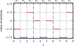
(a) Control parameters
$\alpha=(-\frac{\pi}{4},-\frac{\pi}{2},\frac{\pi}{4},0,-\frac{\pi}{2},0,-\frac{\pi}{4},-\frac{\pi}{2},\frac{\pi}{4})$.

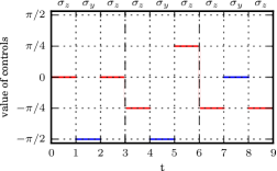
(b) Control parameters
$\alpha=(0,-\frac{\pi}{2},0,-\frac{\pi}{4},-\frac{\pi}{2},\frac{\pi}{4},-\frac{\pi}{4},0,-\frac{\pi}{4})$.

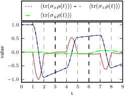
(c) Mean values of $\sigma_{x},\sigma_{y}$ and $\sigma_{z}$.

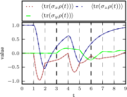
(d) Mean values of $\sigma_{x},\sigma_{y}$ and $\sigma_{z}$.

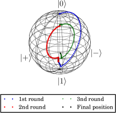
(e) Time evolution of a quantum coin.

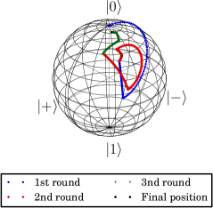
(f) Time evolution of a quantum coin.

Figure 1: Example of the time evolution of a quantum system with the amplitude damping decoherence for a sequence of control parameters $\alpha$ and fixed $\gamma=0.1$ (left side), $\gamma=0.7$ (right side).

The noisy operator $\sigma_{+}$ is related to amplitude raising decoherence, and the solution of the master equation has the following form

$$\rho(t)=e^{At}\rho(0)e^{A^{\dagger}t}-e^{-\gamma t}\sigma_{+}\rho(0)\sigma_{-},$$ (11)

where $A=-\mathrm{i}H(t)-\frac{1}{2}\gamma\sigma_{-}\sigma_{+}$. It is easy to check that as $\gamma\rightarrow\infty$ the state $|1\rangle\langle 1|$ is the solution of the above equation, in which case Alice wins.

3.2 Phase damping

Now we consider the impact of the phase damping decoherence on the outcome of the game. In this case, the Lindblad operator is given by $\sigma_{z}$. Hence, the Lindblad equation has the following form

$$\frac{\mathrm{d}\rho}{\mathrm{d}t}=-\mathrm{i}[H,\rho]+\gamma(\sigma_{z}\rho\sigma_{z}-\frac{1}{2}\sigma_{z}\sigma_{z}\rho-\frac{1}{2}\rho\sigma_{z}\sigma_{z})=-\mathrm{i}[H,\rho]+\gamma(\sigma_{z}\rho\sigma_{z}-\rho).$$ (12)

Next, we make a change of variables $\hat{\rho}(t)=e^{\mathrm{i}Ht}\rho(t)e^{-\mathrm{i}Ht}$, which is helpful to solve the equation. We obtain

$$\frac{\mathrm{d}\hat{\rho}}{\mathrm{d}t}=\gamma(\sigma_{z}\hat{\rho(t)}\sigma_{z}-\hat{\rho(t)}).$$ (13)

It follows that the solution of the above equation is given by

$$\begin{split}\hat{\rho}(t)=&|0\rangle\langle 0|\rho(0)|0\rangle\langle 0|+|1\rangle\langle 1|\rho(0)|1\rangle\langle 1|+\\ +&\mathrm{e}^{-2\gamma t}(|0\rangle\langle 0|\rho(0)|1\rangle\langle 1|+|1\rangle\langle 1|\rho(0)|0\rangle\langle 0|).\end{split}$$ (14)

Coming back to the original variables we get the expression

$$\begin{split}\rho(t)=&|0\rangle\langle 0|\rho(0)|0\rangle\langle 0|+|1\rangle\langle 1|\rho(0)|1\rangle\langle 1|+\\ +&\mathrm{e}^{-2\gamma t}\mathrm{e}^{-\mathrm{i}Ht}(|0\rangle\langle 0|\rho(0)|1\rangle\langle 1|+|1\rangle\langle 1|\rho(0)|0\rangle\langle 0|)\mathrm{e}^{\mathrm{i}Ht}.\end{split}$$ (15)

Consider the following limit

$$\lim_{\gamma\to\infty}\rho(t)=|0\rangle\langle 0|\rho(0)|0\rangle\langle 0|+|1\rangle\langle 1|\rho(0)|1\rangle\langle 1|.$$ (16)

The above result is a diagonal matrix dependent on the initial state. For high values of $\gamma$, the initial state $\rho(0)$ has a significant impact on the game. If $\rho(0)=|0\rangle\langle 0|$ then $\lim_{\gamma\to\infty}\rho(t)=|0\rangle\langle 0|$. This kind of decoherence is conducive to Bob. Similarly, if $\rho(0)=|1\rangle\langle 1|$, then Alice wins. The evolution of a quantum system with the phase damping decoherence and fixed Hamiltonian is shown in Figure 2.

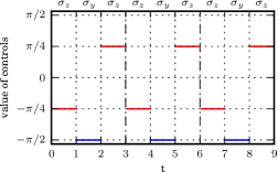
(a) Control parameters
$\alpha=(-\frac{\pi}{4},-\frac{\pi}{2},\frac{\pi}{4},-\frac{\pi}{4},-\frac{\pi}{2},\frac{\pi}{4},-\frac{\pi}{4},-\frac{\pi}{2},\frac{\pi}{4})$.

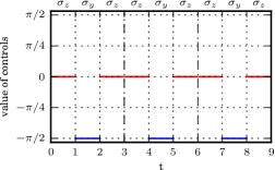
(b) Control parameters
$\alpha=(0,-\frac{\pi}{2},0,0,-\frac{\pi}{2},0,0,-\frac{\pi}{2},0)$.

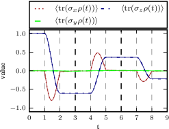
(c) Mean values of $\sigma_{x},\sigma_{y}$ and $\sigma_{z}$.

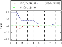
(d) Mean values of $\sigma_{x},\sigma_{y}$ and $\sigma_{z}$.

(e) Time evolution of a quantum coin.

(f) Time evolution of a quantum coin.

Figure 2: Example of the time evolution of a quantum system with the phase damping decoherence for fixed $\gamma=0.5$ (left side), $\gamma=5$ (right side) and a sequence of control parameters $\alpha$.

4 Optimal strategy for the players

Due to the noisy evolution of the underlying qubit, the strategy given by Table 2 is no longer a Nash equilibrium. We study the possibility of optimizing one player’s strategy, while the other one uses the Pauli strategy. It turns out that this optimization is not always possible. If the rate of decoherence is high enough, then the players’ strategies have little impact on the game outcome. In the low noise scenario, it is possible to optimize the strategy of both players.

In each round, one player performs a series of unitary operations, which are chosen randomly from a uniform distribution. Therefore, the strategy of a player can be seen as a random unitary channel. In this section $\Phi_{A_{1}},\Phi_{A_{2}}$ denote mixed unitary channels used by Alice who implements the Pauli strategy. Similarly, $\Phi_{B}$ denotes channels used by Bob.

4.1 Optimization method

In order to find optimal strategies for the players we assume the Hamiltonian in (3) to have the form

$$H=H(\varepsilon(t)),$$ (17)

where $\varepsilon(t)$ are the control pulses. As the optimization target, we introduce the cost functional

$$J(\varepsilon)=\mathrm{tr}\{F_{0}(\rho(T))\},$$ (18)

where $F_{0}(\rho(T))$ is a functional that is bounded from below and differentiable with respect to $\rho(T)$. A sequence of control pulses that minimizes the functional (18) is said to be optimal. In our case we assume that

$$\mathrm{tr}\{F_{0}(\rho(T))\}=\frac{1}{2}||\rho(T)-\rho_{\rm T}||_{\rm F}^{2},$$ (19)

where $\rho_{\rm T}$ is the target density matrix of the system.

In order to solve this optimization problem, we need to find an analytical formula for the derivative of the cost functional (18) with respect to control pulses $\varepsilon(t)$. Using the Pontryagin principle [15], it is possible to show that we need to solve the following equations to obtain the analytical formula for the derivative [6]

$$\frac{\mathrm{d}\rho(t)}{\mathrm{d}t} =-\mathrm{i}[H(\varepsilon(t)),\rho(t)]-\mathrm{i}L_{\rm D}[\rho(t)],\;t\in[0,T],$$ (20)

$$\frac{\mathrm{d}\lambda(t)}{\mathrm{d}t} =-\mathrm{i}[H(\varepsilon(t)),\lambda(t)]-\mathrm{i}L_{\rm D}^{\dagger}[\lambda(t)],\;t\in[0,T],$$ (21)

$$L_{\rm D}[A] =\mathrm{i}\sum_{j}\gamma_{j}(L_{j}AL_{j}^{\dagger}-\frac{1}{2}\{L_{j}^{\dagger}L_{j},A\}),$$ (22)

$$\rho(0) =\rho_{\rm s},$$ (23)

$$\lambda(T) =F^{\prime}_{0}(\rho(T)),$$ (24)

where $\rho_{\rm s}$ denotes the initial density matrix, $\lambda(t)$ is called the adjoint state and

$$F^{\prime}_{0}(\rho(T))=\rho(T)-\rho_{\rm T}.$$ (25)

In order to optimize the control pulses using a gradient method, we convert the problem from an infinite dimensional (continuous time) to a finite dimensional (discrete time) one. For this purpose, we discretize the time interval $[0,T]$ into $M$ equal sized subintervals $\Delta t_{k}$. Thus, the problem becomes that of finding $\varepsilon=[\varepsilon_{1},\ldots,\varepsilon_{M}]^{\rm T}$ such that

$$J(\varepsilon)=\inf_{\zeta\in\mathbb{R}^{M}}J(\zeta).$$ (26)

The gradient of the cost functional is

$$G=\left[\frac{\partial J}{\partial\varepsilon_{1}},\ldots,\frac{\partial J}{\partial\varepsilon_{M}}\right]^{\rm T}.$$ (27)

It can be shown [6] that elements of vector (27) are given by

$$\frac{\partial J}{\partial\varepsilon_{k}}=\mathrm{tr}\left\{-\mathrm{i}\lambda_{k}\left[\frac{\partial H(\varepsilon_{k})}{\partial\varepsilon_{k}},\rho_{k}\right]\right\}\Delta t_{k},$$ (28)

where $\rho_{k}$ and $\lambda_{k}$ are solutions of the Lindblad equation and the adjoint system corresponding to time subinterval $\Delta t_{k}$ respectively. To minimize the gradient given in Eq. (27) we use the BFGS algorithm [16].

4.2 Optimization setup

Our goal is to find control strategies for players, which maximize their respective chances of winning the game. We study three noise channels: the amplitude damping, the phase damping and the amplitude raising channel. They are given by the Lindblad operators $\sigma_{-}$, $\sigma_{z}$ and $\sigma_{+}=\sigma_{-}^{\dagger}$, respectively. In all cases, we assume that one of the players uses the Pauli strategy, while for the other player we try to optimize a control strategy that maximizes that player’s probability of winning. However, in our setup it is convenient to use the value of the observable $\sigma_{z}$ rather than probabilities. Value 0 means that each player has a probability of $\frac{1}{2}$ of winning the game. Values closer to 1 mean higher probability of winning for Bob, while values closer to -1 mean higher probability of winning for Alice.

4.3 Optimization results

4.3.1 Phase damping

The results for the phase damping channel are shown in Figure 3. As it can be seen, in this case both players are able to optimize their strategies, and so Alice can optimize her strategy for low values of $\gamma$ to obtain the probability of winning grater than $\frac{1}{2}$. The region where this occurs is shown in the inset. For high noise values she is able to achieve the probability of winning equal to $\frac{1}{2}$. On the other hand, optimization of Bob’s strategy shows that he is able to achieve high probabilities of winning for relatively low values of $\gamma$. Figure 4 presents optimal game strategies for both players. For Alice we chose $\gamma=1.172$ which corresponds to her maximal probability of winning the game. In the case of Bob’s strategies we arbitrarily choose the value $\gamma=1.610$.

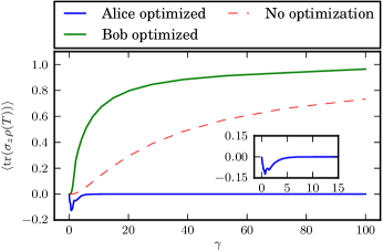
Figure 3: Mean value of the pay-off for the phase damping channel with and without optimization of the player’s strategies. The inset shows the region where Alice is able to increase her probability of winning to exceed $\frac{1}{2}$.

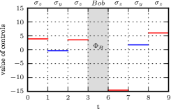
(a) Optimal controls for Alice.

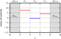
(b) Optimal controls for Bob.

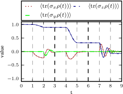
(c) Mean values of $\sigma_{x},\sigma_{y}$ and $\sigma_{z}$.

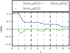
(d) Mean values of $\sigma_{x},\sigma_{y}$ and $\sigma_{z}$.

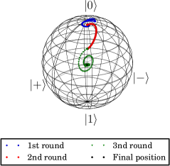
(e) Time evolution of a quantum coin.

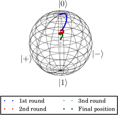
(f) Time evolution of a quantum coin.

Figure 4: Game results for the phase damping channel. Optimal Alice’s strategy when $\gamma=1.172$ (left side), and optimal Bob’s strategy when $\gamma=1.610$ (right side).

4.3.2 Amplitude damping

Next, we present the results obtained for the amplitude damping channel. They are shown in Figure 5. Unfortunately for Alice, for high values of $\gamma$ Bob always wins. This is due to the fact that in this case the state quickly decays to state $|0\rangle\langle 0|$. Additionally, Bob is also able to optimize his strategies. He is able to achieve probability of winning equal to 1 for relatively low values of $\gamma$. For low values of $\gamma$ the interaction allows Alice to achieve higher than $\frac{1}{2}$ probability of winning. The region where this happens is magnified in the inset. Interestingly, for very low values of $\gamma$ Alice can increase her probability of winning. This is due to the fact, that low noise values are sufficient to distort Bob’s attempts to perform the Pauli strategy. On the other hand, they are not high enough to drive the system towards state $|0\rangle\langle 0|$. Optimal game results for both players are shown in Figure 6. For both players we chose $\gamma=0.621$ which corresponds to Alice’s maximal probability of winning the game.

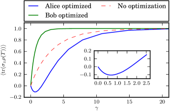
Figure 5: Mean value of the pay-off for the amplitude damping channel with and without optimization of the player’s strategies. The inset shows the region where Alice is able to increase her probability of winning to exceed $\frac{1}{2}$.

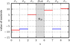
(a) Optimal controls for Alice.

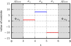
(b) Optimal controls for Bob.

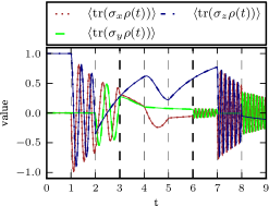
(c) Mean values of $\sigma_{x},\sigma_{y}$ and $\sigma_{z}$.

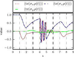
(d) Mean values of $\sigma_{x},\sigma_{y}$ and $\sigma_{z}$.

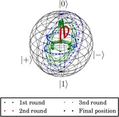
(e) Time evolution of a quantum coin.

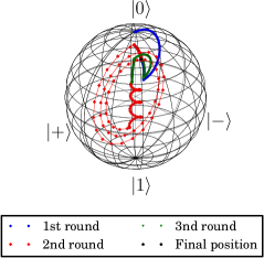
(f) Time evolution of a quantum coin.

Figure 6: Game results obtained for the amplitude damping channel with $\gamma$ equal to $0.621$. Optimal Alice’s strategy (left side), and optimal Bob’s strategy (right side).

4.3.3 Amplitude raising

Finally, we present optimization results for the amplitude raising channel. The optimization results, shown in Figure 7, indicate that Alice can achieve probability of winning equal to 1 for lower values of $\gamma$ compared to the unoptimized case. In this case Bob cannot do any better than in the unoptimized case due to a limited number of available control pulses.

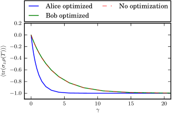
Figure 7: Mean value of the pay-off for the amplitude raising channel with and without optimization of the player’s strategies.

5 Conclusions

We studied the quantum version of the coin flip game under decoherence. To model the interaction with external environment we used the Markovian approximation in the form of the Lindblad equation. Because of the fact that Pauli strategy is a known Nash equilibrium of the game, therefore it was natural to investigate this strategy in the presence noise. Our results show that in the presence of noise the Pauli strategy is no longer a Nash equilibrium. One of the players, Bob in our case, is always favoured by amplitude and phase damping noise.

Our next step was to check if the players were able to do better than the Pauli strategy. For this, we used the BFGS gradient method to optimize the players’ strategies. Our results show that Alice, as well as Bob, are able to increase their respective winning probabilities. Alice can achieve this for all three studied cases, while Bob can only do this for the phase damping and amplitude damping channels.

References

- [1] J.-L. Chen, L. Kwek, and C. Oh. Noisy quantum game. Physical Review A, 65(5):052320, 2002.
- [2] A.P. Flitney and L.C.L. Hollenberg. Multiplayer quantum minority game with decoherence. In Proceedings of SPIE, volume 5842, pages 175–182, 2005.
- [3] P. Gawron. Noisy Quantum Monty Hall Game. Fluctuation and Noise Letters, 9(1):9–18, 2010.
- [4] P. Gawron, J.A. Miszczak, and J. Sładkowski. Noise effects in quantum magic squares game. International Journal of Quantum Information, 6(supp01):667–673, 2008.
- [5] T. Heinosaari and M. Ziman. The mathematical language of quantum theory: from uncertainty to entanglement. Cambridge University Press, 2011.
- [6] H. Jirari and W. Pötz. Optimal coherent control of dissipative -level systems. Physical Review A, 72(1):013409, 2005.
- [7] N.F. Johnson. Playing a quantum game with a corrupted source. Physical Review A, 63(2):20302, 2001.
- [8] S. Khan, M. Ramzan, and M. K. Khan. Quantum Monty Hall problem under decoherence. Communications in Theoretical Physics, 54(1):47, 2010.
- [9] J.A. Miszczak, P. Gawron, and Z. Puchała. Qubit flip game on a Heisenberg spin chain. Quantum Information Processing, 11(6):1571–1583, 2012.
- [10] A. Nawaz. Prisoners’ dilemma in the presence of collective dephasing. Journal of Physics A: Mathematical and Theoretical, 45(19):195304, 2012.
- [11] M. A. Nielsen and I. L. Chuang. Quantum Computation and Quantum Information. Cambridge University Press, 2000.
- [12] I. Pakuła. Analysis of trembling hand perfect equilibria in quantum games. Fluctuation and Noise Letters, 8(01):23–30, 2008.
- [13] Łukasz Pawela, Piotr Gawron, Zbigniew Puchała, and Jan Sładkowski. Enhancing pseudo-telepathy in the magic square game. PLoS ONE, 8(6):e64694, 2013.
- [14] E.W. Piotrowski and J. Sładkowski. An invitation to quantum game theory. International Journal of Theoretical Physics, 42(5):1089–1099, 2003.
- [15] L. S. Pontryagin, V. G. Boltyanskii, R. V. Gamkrelidze, and E. Mishchenko. The mathematical theory of optimal processes. Interscience Publishers, 1962.
- [16] W.H. Press, B.P. Flannery, S.A. Teukolsky, and W.T. Vetterling. Numerical Recipes in FORTRAN 77, volume 1 of Fortran Numerical Recipes: The Art of Scientific Computing. Cambridge University Press, 1992.