Probing modified gravity theories with the Sandage-Loeb test

Abstract

In this paper, we quantify the ability of a future measurement of the Sandage-Loeb test signal from the Cosmic-Dynamic-Experiment-like spectrograph to constrain some popular modified gravity theories including the Dvali-Gabadadze-Porrati braneworld scenario, $f(R)$ modified gravity and $f(T)$ gravity theory. We find that the Sandage-Loeb test measurements are able to break degeneracies between model parameters markedly and thus greatly improve cosmological constraints for all concerned modified gravity theories when combined with the latest observations of CMB–shift parameter. However, they yield almost the same degeneracy directions between model parameters as that from the distance ratio data derived from the latest observations of the cosmic microwave background and baryonic acoustic oscillations. Moreover, for the $f(R)$ modified gravity, the Sandage-Loeb test could provide completely different bounded regions in model parameters space as compared to CMB/BAO and thus supplement strong complementary constraints.

I INTRODUCTION

In the past decade or so, an accelerating expanding universe was first indicated by observations of type Ia supernova (SNe Ia) Riess0 ; Perlmutter and subsequently confirmed by several other surveys such as the cosmic microwave background (CMB) CMB , and baryonic acoustic oscillation (BAO) BAO . This ostensibly counterintuitive behavior of the universe is usually attributed to a presently unknown component, called dark energy, which exhibits negative pressure and dominates over the matter-energy content of our universe. So far, the simplest candidate for dark energy is the cosmological constant and the standard cosmological model based on it (dubbed $\Lambda$CDM) is in accordance with almost all the existing cosmological observations. However, dark energy is not the only explanation for the current cosmic acceleration, modified gravity theories in which gravitational interaction deviates from Einstein’s theory of gravity can also account for this apparently unusual phenomenon. So far, both models derived from introducing an exotic component like dark energy and those established by modifying Einstein’s theory of gravity can survive the above-mentioned observations. If one wants to place more comprehensive cosmological constraints on a possible model or distinguish between dark energy and modified gravity theories, it is crucial to measure the expansion rate of universe at many different redshifts. Among the known probes, the CMB probes the rate of the expansion at redshift $z\sim 1100$, while for much lower redshift ($z\leqslant 2$) we could rely on weak lensing, BAOs, and the most noticeably, luminosity distance measurements of SNe Ia and some other probes. In particular, a new cosmological window would open if we could measure the cosmic expansion directly within the “redshift desert”, roughly corresponding to redshifts $2\leqslant z\leqslant 5$.

Currently, the detailed dynamics of the accelerated expansion is still not well known. However, one could expect the redshift of any given object to exhibit a specific time evolution in an underlying cosmological model. The observation of this evolution performed over a given time interval could not only be a direct probe of the dynamics of the expansion, but also has the advantage of not depending on a determination of the absolute luminosity of the observed source. Allan Sandage first proposed the possible application of this kind of observation as a cosmological tool Sandage . However, only measurements performed at time interval separated by more than $10^{7}$ years could have detected the cosmic signal with the technology at available that time. Over the past decades, the importance of this method was stressed again Rudiger ; Lake . Later, Loeb revisited these ideas and argued that spectroscopic techniques developed for detecting the reflex motion of stars induced by unseen orbiting planets could be used to detect the redshift variation of quasar stellar object (QSO) Lyman-$\alpha$ absorption line Loeb . He also concluded that it is conceivable that the cosmological redshift variation in the spectra of some suitable source could be detected in a few decades. Therefore, this method is usually referred as the “Sandage-Loeb” (SL) test. More recently, by using the Green Bank Telescope (GBT) observation over 13.5 years, precise measurements for the secular redshift drift of 10 HI 21 cm absorption line systems spanning $z=0.09-0.69$ were obtained Darling . These surveys were announced as direct measurements of the cosmic acceleration and an error-weighted mean secular redshift drift of $<\dot{z}>=(-2.3\pm 0.8)\times 10^{-8}~{}\mathrm{yr}^{-1}$, corresponding to an acceleration of $<\dot{v}>=-5.5\pm 2.2~{}\mathrm{m}\cdot\mathrm{s}^{-1}\cdot\mathrm{yr}^{-1}$, was achieved. Encouragingly, the cosmic acceleration could be directly measured in $\sim 125$ years with current telescopes or in $\sim 5$ years using a Square Kilometer Array .

An investigation of the expected cosmological constraints from the SL test for a constant dark energy equation of state was performed by Corasaniti et al. Corasaniti . Later, several extended analysis for some other popular competing models including Chaplygin gas, holographic dark energy and the new agegraphic and Ricci dark energy Balbi ; Hongbao ; Jinfei , were accomplished. More recently, the ability of a future measurement of the SL signal from a Cosmic-Dynamics-Experiment-like (CODEX) CODEX spectrograph to constrain a dynamical dark energy (CPL parametrization CPL ) was quantified by Martinelli et al. Martinelli . Alongside the full CMB mock data set with noise properties consistent with Plank-like Plank experiment, they demonstrated that the SL test measurements could be able to break degeneracies between expansion parameters and improve cosmological constraints greatly.

In this paper, we perform, along the line of Ref. Martinelli , a joint analysis by taking the latest observations of CMB–shift parameter into account to investigate the constraining power of the SL test on model parameters of modified gravity theories including the Dvali-Gabadadze-Porrati (DGP) brane-world scenario DGP , the $f(R$) gravity (see Refs. FR1 ; FR2 for recent reviews) and the $f(T$) gravity FT . Moreover, analysis with the distance ratios derived from the latest CMB and BAO observations (labeled as CMB/BAO), which are deemed to be more suitable than the primitive CMB data for examining non-standard dark energy models, are also taken into consideration for comparison.

II DATA SETS

In this section, we give brief descriptions for the data sets.

II.1 Sandage-Loeb Test

We begin with reviewing the basic theory necessary to derive the expected redshift drift over a time interval in a given cosmological model. In a Friedmann-Lemaître-Robertson-Walker (FLRW) expanding universe, the radiation emitted by a source which does not possess any peculiar motion at time $t_{s}$ and observed at time $t_{0}$ experiences a redshift $z_{s}$ which is connected to the expansion rate through the scale factor $a(t)$ as

$$1+z_{s}(t_{0})=\frac{a(t_{0})}{a(t_{s})}.$$ (1)

After a time interval $\Delta t_{0}$ (corresponding to $\Delta t_{s}$ for the source), it becomes

$$1+z_{s}(t_{0}+\Delta t_{0})=\frac{a(t_{0}+\Delta t_{0})}{a(t_{s}+\Delta t_{s})}.$$ (2)

With an adequate time interval between observations, we can measure the observed redshift variation

$$\Delta z_{s}=\frac{a(t_{0}+\Delta t_{0})}{a(t_{s}+\Delta t_{s})}-\frac{a(t_{0})}{a(t_{s})}.$$ (3)

By keeping the first order in $\Delta t/t$, this difference can be re-written as

$$\Delta z_{s}\simeq\Delta t_{0}\bigg{[}\frac{\dot{a}(t_{0})-\dot{a}(t_{s})}{a(t_{s})}\bigg{]}.$$ (4)

Conveniently, this redshift variation is usually expressed in terms of a spectroscopic velocity shift, i.e.,

$$\Delta v=\frac{c\Delta z_{s}}{1+z_{s}},$$ (5)

where $c$ is the speed of light. Therefore, the velocity variation can be related to the matter-energy content of the universe by setting $a(t_{0})=1$ and using the Friedmann equation,

$$\frac{\Delta v}{c}=H_{0}\Delta t_{0}\bigg{[}1-\frac{E(z_{s})}{1+z_{s}}\bigg{]},$$ (6)

where $H_{0}$ is the Hubble constant and $E(z)=H(z)/H_{0}$.

The feasibility of detecting a time evolution of the redshift was once studied in detail by Pasquini et al. Pasquini1 ; Pasquini2 . The most promising system used to measure the velocity shift within the redshift desert is quasar absorption lines typical of the Lyman-$\alpha$ forest. The European Extremely Large Telescope with a high-resolution ultra-stable spectrograph such as CODEX will be able to detect the tiny shift in spectral line over a reasonable time interval, typically of the order of few decades EELT .

According to the latest Monte Carlo simulations, the accuracy of the spectroscopic velocity shift measurements expected by CODEX can be expressed as

$$\sigma_{\Delta_{v}}=1.35\frac{2370}{S/N}\sqrt{\frac{30}{N_{\mathrm{QSO}}}}\bigg{(}\frac{5}{1+z_{\mathrm{QSO}}}\bigg{)}^{x}~{}\mathrm{cm}~{}\mathrm{s}^{-1},$$ (7)

where $S/N$ is the signal-to-noise ratio, $N_{\mathrm{QSO}}$ is the number of observed quasars, $z_{\mathrm{QSO}}$ represent their redshift and the index $x$ is 1.7 for $z\leqslant 4$ while it becomes 0.9 beyond that redshift. The mock SL data set used in our following analysis corresponds to the error bars computed from Eq. (7) with a $S/N$ of 3000 and a number of QSO $N_{\mathrm{QSO}}=30$ assumed to be uniformly distributed among the following redshift bins: $z_{\mathrm{QSO}}=[2.0,2.5,3.0,3.5,4.0,4.5,5.0]$. The fiducial concordance cosmological model with the parameters taken to be the best-fit ones from WMAP nine years analysis WMAP9 is applied to examine the capacity of future measurements of SL test to constrain the concerned models

II.2 The Cosmic Microwave Background and Baryonic Acoustic Oscillations

There are two useful parameters commonly employed when analyzing the CMB observations. One describes the scaled distance to recombination, $\mathcal{R}$, and the other the angular scale of the sound horizon at recombination, $\ell_{A}$ Komatsu ; Elgaroy ; Wang .

The shift parameter $\mathcal{R}$ is defined as

$$\mathcal{R}=\sqrt{\Omega_{m}}\int_{0}^{z_{*}}\frac{dz}{E(z)},$$ (8)

where $z_{*}\sim 1091$ is the redshift of the last-scattering surface.

The position of the first CMB power-spectrum peak, which corresponds to the angular scale of the sound horizon at recombination, is given by

$$\ell_{A}=\pi\frac{d_{A}(z_{*})}{r_{s}(z_{*})},$$ (9)

where $d_{A}$ is the comoving angular diameter distance, $r_{s}(z_{*})$ is the comoving sound horizon at recombination

$$r_{s}(z_{*})=\int_{z_{*}}^{\infty}\frac{c_{s}}{H(z)}dz$$ (10)

which is dependent on the speed of sound, $c_{s}$, in the early universe. Using both these two parameters in combination reproduces closely the fit from the full CMB power spectrum and it was shown that constraints from the shift parameter $\mathcal{R}$ alone could approximately represent the degeneracy directions between model parameters from the full CMB observations Elgaroy .

In our analysis, the data based on measurements of the CMB acoustic scale WMAP9

$$\ell_{A}=302.35\pm 0.65$$ (11)

and the ratios of the sound horizon scale at the drag epoch ($z_{d}\sim 1021$) to the BAO dilation scale BAO2

$$\begin{split}\frac{r_{s}(z_{d})}{D_{V}(z=0.20)}&=0.1905\pm 0.0061&\\ \frac{r_{s}(z_{d})}{D_{V}(z=0.35)}&=0.1097\pm 0.0036&\\ \frac{r_{s}(z_{d})}{D_{V}(z=0.44)}&=0.0916\pm 0.0071&\\ \frac{r_{s}(z_{d})}{D_{V}(z=0.60)}&=0.0726\pm 0.0034&\\ \frac{r_{s}(z_{d})}{D_{V}(z=0.73)}&=0.0592\pm 0.0032&\end{split}$$ (12)

where the so-called dilation scale, $D_{V}$, is given by

$$D_{V}(z)=\bigg{[}(1+z)^{2}d_{A}^{2}\frac{cz}{H(z)}\bigg{]}^{1/3},$$ (13)

are also taken into account to study the constraining power of SL test.

By considering the ratio of the sound horizons at drag epoch and photon decoupling, $r_{s}(z_{d})/r_{s}(z_{*})=1.045\pm 0.012$ WMAP9 , and combining the observational results of (11) and (12), we obtain

$$\begin{split}f_{0.20}=\frac{d_{A}(z_{*})}{D_{V}(z=0.20)}&=17.55\pm 0.60&\\ f_{0.35}=\frac{d_{A}(z_{*})}{D_{V}(z=0.35)}&=10.11\pm 0.35&\\ f_{0.44}=\frac{d_{A}(z_{*})}{D_{V}(z=0.44)}&=8.44\pm 0.66&\\ f_{0.60}=\frac{d_{A}(z_{*})}{D_{V}(z=0.60)}&=6.69\pm 0.32&\\ f_{0.73}=\frac{d_{A}(z_{*})}{D_{V}(z=0.73)}&=5.45\pm 0.30.&\end{split}$$ (14)

In addition, the coefficients $0.337$, $0.369$ and $0.438$ which correlate the pairs of measurements at $z=(0.20,0.35)$, $z=(0.44,0.60)$ and $z=(0.60,0.73)$ respectively are taken into consideration in our analysis. It should be stressed that these distance ratios is deemed to could provide more reasonable constraints on non-standard dark energy models than the primitive CMB or BAOs data Sollerman ; Zheng .

III MODELS AND RESULTS

In the last two decades or so, numerous models have been proposed to explain the observed cosmic acceleration. Although some models may be preferred with respect to others based on some statistical assessment as they fit the data better with a small number of parameters Davis ; Sollerman ; Zheng , most of them have not been falsified by available tests of the background cosmology. These models can be classified in two categories: (1)Models based on an exotic component dubbed dark energy; (2)Models based on modified gravity in which gravitational interaction deviates from Einstein’s theory of gravity. Examples of the latter include DGP brane-world scenario DGP , $f(R$) gravity FR and $f(T$) gravity FT . The SL test has been applied to explore dark energy in the past few years Corasaniti ; Balbi ; Hongbao ; Jinfei . In this paper, we focus on the time evolution of the cosmological redshift as a test of modified gravity theories, including the predictions on the time evolution of the velocity shift derived from observations performed over a time interval $\Delta t_{0}=30~{}\mathrm{yr}$ and the constraints on model parameters from a future CODEX-like SL signal.

III.1 DGP model

The DGP model DGP , which provides a mechanism for accelerated expansion without introducing a repulsive-gravity fluid, arises from a class of brane-world scenario in which gravity leaks out into the bulk above a certain cosmologically relevant physical scale. This leaking of gravity is responsible for the increase in the expansion rate with time. In the framework of a spatially flat DGP model, the Friedmann equation is modified as

$$H^{2}-\frac{H}{r_{c}}=\frac{8\pi G}{3}\rho_{m},$$ (15)

where $r_{c}=1/[H_{0}(1-\Omega_{m})]$, which represents the critical length scale beyond which gravity leaks out into the bulk. In this paper, we investigate the generalized DGP model DGP2 , which interpolates between the pure $\Lambda$CDM and original DGP model with an additional parameter $\lambda$,

$$H^{2}-\frac{H^{\lambda}}{r_{c}^{2-\lambda}}=\frac{8\pi G}{3}\rho_{m},$$ (16)

where $r_{c}=1/[H_{0}(1-\Omega_{m})^{\lambda-2}]$. Thus, we can directly rewrite the above equation and obtain the expansion rate

$$E^{2}(z)=\frac{H^{2}}{H_{0}^{2}}=\Omega_{m}(1+z)^{3}+(1-\Omega_{m})E^{\lambda}(z).$$ (17)

For $\lambda=1$, this agrees with the original DGP Friedmann-like equation, while $\lambda=0$ leads to an expansion history identical to that of standard $\Lambda$CDM cosmology. The cosmological constraints on this generalized scenario from current observations were presented in detail in Ref. junqing .

The predications on the time evolution of the velocity shift over a time interval $\Delta t_{0}=30~{}\mathrm{yr}$ for the DGP model are shown in Fig. (1). Compared to simulated data as expected from the CODEX experiment in a fiducial concordance $\Lambda$CDM model with the parameters taken to be the best-fit ones from WMAP nine years analysis WMAP9 , the DGP model with $\Omega_{m}\sim[0.23,0.27]$ and $\lambda\sim[-0.2,0.6]$ seems to be favored. Alongside the primitive CMB–shift parameter or CMB/BAO, the ability of a future SL signal measurement to constrain this model is presented in Fig. (2). From the left panel of this Figure, we find that the SL test is able to break the degeneracies between model parameters when combined with the CMB–shift parameter data and thus greatly improve cosmological constraints. This is similar to what was obtained for a CPL-like dynamical dark energy Martinelli . However, as shown in the right panel, the advantage disappears when the CMB–shift parameter is replaced by CMB/BAO. Nevertheless, in either case, the SL test imposes a strong bound on $\Omega_{m}$, which is similar to what was obtained when the holographic dark energy model was explored with the SL test Hongbao .

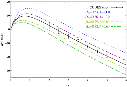
Figure 1: The predicted velocity shift over a time interval $\Delta t_{0}=30~{}\mathrm{yr}$ for the DGP model, compared to simulated data as expected from the CODEX experiment. The mock data points and error bars are estimated from Eq. (7) with a fiducial concordance $\Lambda$CDM model.

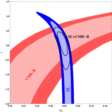
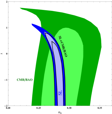
Figure 2: $\mathrm{\mathbf{Left}}$: Constraints on the DGP model using SL test (blue layer), CMB–shift parameter (red layer), and combining the two probes (black solid lines). $\mathrm{\mathbf{Right}}$: Constraints on the DGP model using SL test (blue layer), CMB/BAO (green layer), and combining the two probes (black solid lines).

III.2 $f(R$) modified gravity

The $f(R$) gravity theories modify general relativity by introducing nonlinear generalizations to the (linear) Hilbert action (see Refs. FR1 ; FR2 for recent reviews). As the generalized Lagrangians of this type can lead to accelerating phases both at early Starobinsky and late Capozziello1 ; Carroll times in the history of the universe (see also Ref. Capozziello3 ; Nojiri ), a great deal of interest and effort has gone into the study of such theories.

The starting point of the $f(R$) theories in the Palatini approach is the Einstein-Hilbert action, which is given by

$$S=\int d^{4}x\sqrt{-g}\bigg{[}\frac{1}{2k}f(R)+\mathcal{L}_{m}\bigg{]},$$ (18)

where $f$ is a differentiable function of the Ricci scalar $R$, $\mathcal{L}_{m}$ is the Lagrangian of the pressureless matter, $k=8\pi G$, and $G$ is the gravitational constant. For a flat Friedmann-Lemaître-Robertson-Walker (FLRW) background, the Hubble parameter in terms of the curvature scalar $R$ reads

$$H^{2}=\frac{2k\rho_{m}+FR-f}{6F\xi},$$ (19)

where

$$\xi=\bigg{[}1-\frac{3F^{\prime}(FR-2f)}{2F(F^{\prime}R-F)}\bigg{]}^{2},$$ (20)

and $F=\partial f/\partial R$ and a prime denotes a derivative with respect to $R$. In the case of the Hilbert action with $f=R$, Eq. (19) reduces to the standard Friedmann equation: $H^{2}=k\rho_{m}/3$. In this paper, we adopt the $f(R$) gravity theory with the form $f(R)=R-\alpha(-R)^{\beta}$ within the Palatini approach which can not only pass the solar system test and has the correct Newtonian limit Sotiriou , but also can explain the late accelerating phase of the expansion. Constraints from observations such as the CMB–shift parameter, SNe Ia surveys data, BAOs, the matter power spectrum from the SDSS and gravitational lensing on this type of $f(R$) theory have been intensively discussed Santos ; Fay ; Borowiec ; Amarzguioui ; Sotiriou06a ; Koivisto ; LiB ; DMchen ; kai . Here, we evaluate the constraining power on this class of $f(R$) gravity theory from a future measurement of SL test.

The predications on the time evolution of the velocity shift and the numerical results which demonstrate the ability of a future SL signal measurement to constrain this modified gravity theory are shown in Fig. (3) and Fig. (4) respectively. The results shown in the left panel of Fig. (4) suggest that the degeneracies between model parameters $\alpha$ and $\beta$ could be broken by including the SL test when the observations of CMB–shift parameter is considered. However, as shown in the right panel, we find that the constraints from the SL test and the CMB/BAO present almost the same directions of degeneracy between model parameters. This means that, alongside the CMB/BAO, the SL test is not capable of breaking the existing degeneracy between model parameters.

It is interesting to note that the bounded regions in the $\alpha-\beta$ plane from these two data sets are clearly different, i.e., there is no overlap at 95.4% confidence level (C. L.). Therefore the SL test can provide complementary constraints on the model parameters as compared to CMB/BAO, and the $\Lambda$CDM ($\beta=0$) might be ruled out at 95.4% C. L. by the joint analysis.

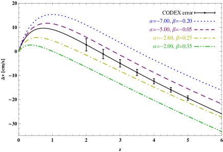
Figure 3: The predicted velocity shift over a time interval $\Delta t_{0}=30~{}\mathrm{yr}$ for the model based on $f(R$) gravity, compared to simulated data as expected from the CODEX experiment. The mock data points and error bars are estimated from Eq. (7) with a fiducial concordance $\Lambda$CDM model.

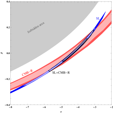
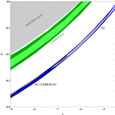
Figure 4: $\mathrm{\mathbf{Left}}$: Constraints on the $f(R)$ gravity using SL test (blue layer), CMB–shift parameter (red layer), and combining the two probes (black solid lines). $\mathrm{\mathbf{Right}}$: Constraints on the $f(R)$ gravity using SL test (blue layer), CMB/BAO (green layer), and combining the two probes (black solid lines).

III.3 $f(T$) gravity

Recently, another kind of modified gravity, named $f(T)$ theory, which can also explain the accelerating cosmic expansion, has attracted an increasing deal of attention. In analogy to the $f(R)$ gravity, the $f(T)$ theory is obtained by extending the action of teleparallel gravity which is based on teleparallel geometry where the spacetime has only torsion and is curvature-free Einstein2 ; Hayashi1 ; Hayashi2 .

Assuming a flat FLRW metric, the expansion rate in terms of torsion scalar $T$ is expressed as

$$H^{2}=\frac{1}{6}\big{[}2k\rho-f+2Tf_{T}\big{]},$$ (21)

where the subscript $T$ represents a derivative with respect to $T$ and $\rho$ is the energy density. Recently, several specific models based on $f(T)$ theory have been proposed Bengochea1 ; Linder . Some of them can not only explain the observed cosmic acceleration, but also can provide an alternative to early inflation Ferraro1 ; Ferraro2 . Observational constraints and some important properties for these models were extensively studied in the last few years Yang ; Wu1 ; Wu2 ; Bengochea2 ; Chen ; Rzheng ; Bamba1 . In this paper, we explore the $f(T)$ gravity theory with the SL test by adopting a model, with the form $f(T)=\alpha(-T)^{n}\tanh\frac{T_{0}}{T}$, in which the phantom divide line crossing might be realized Wu3 . The fundamental requirement $\rho_{\mathrm{eff}}>0$ demands that the parameter $n$ must be greater than $3/2$.

The predications on the time evolution of the velocity shift and the numerical results which represent the ability of a future SL signal measurement to constrain this modified gravity theory are shown in Fig. (5) and Fig. (6) respectively. The same as for the two previously investigated modified gravity theories, the SL test has a strong constraining power on the model parameters and greatly improve the cosmological constraints when combined with the CMB–shift parameter data in the sense that it can break the degeneracies between model parameters. However, this constraining power disappears when the CMB–shift parameter is replaced by the CMB/BAO.

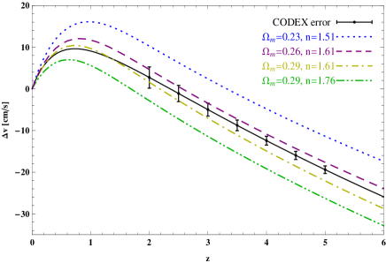
Figure 5: The predicted velocity shift over a time interval $\Delta t_{0}=30~{}\mathrm{yr}$ for the model based on $f(T$) gravity, compared to simulated data as expected from the CODEX experiment. The mock data points and error bars are estimated from Eq. (7) with a fiducial concordance $\Lambda$CDM model.

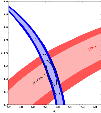
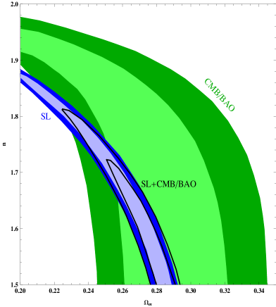
Figure 6: $\mathrm{\mathbf{Left}}$: Constraints on the $f(T)$ gravity using SL test (blue layer), CMB–shift parameter (red layer), and combining the two probes (black solid lines). $\mathrm{\mathbf{Right}}$: Constraints on the $f(T)$ gravity using SL test (blue layer), CMB/BAO (green layer), and combining the two probes (black solid lines).

IV CONCLUSION

In this paper, we have evaluated the power of direct measurements of temporal shift of cosmic redshift of the quasar spectra at sufficiently separated epochs, i.e., the Sandage-Loeb (SL) test, on constraining some popular modified gravity theories including DGP, $f(R)$ modified gravity and $f(T)$ gravity theory. By considering the signal from the Cosmic-Dynamic-Experiment-like spectrograph, we quantify the ability of a future measurement of SL test to constrain these modified gravity theories. Alongside the latest observations of CMB–shift parameter, the SL test measurements are able to break degeneracies between model parameters markedly and thus greatly improve cosmological constraints for all investigated modified gravity theories. This is similar to the constraining power of the SL test on the phenomenological dynamic dark energy model with the CPL parametrization Martinelli . In addition, the distance ratios derived from the latest observations of the cosmic microwave background and baryonic acoustic oscillations (CMB/BAO), which are regarded to be more suitable than the primitive CMB–shift parameter for testing non-standard dark energy models, are taken into consideration for comparison. We find that the SL test measurements and CMB/BAO yield almost the same directions of degeneracy between model parameters for the concerned modified gravity theories. That is, the inclusion of the SL test could not markedly improve the constraints on these three modified gravity theories in terms of degeneracy-breaking of model parameters when the CMB/BAO is considered. However, for the DGP brane-world scenario and $f(T)$ gravity theory, due to a better sensitivity of the SL test, an obvious improvement of constraint on the parameter $\Omega_{m}$ is achieved, which is similar to what was obtained when the holographic dark energy model was explored with the SL test Hongbao . This advantage, of course, might result from the absence of systematic effects which play a key role in the measurement of expansion parameters. For the $f(R)$ modified gravity, the SL test can provide completely different bounded regions in model parameters space as compared to the CMB/BAO, and thus supplement strong complementary constraints.

References

- (1) A. G. Riess et al., AJ, 116, 1009 (1998).
- (2) S. Perlmutter et al., ApJ, 517, 565 (1999).
-
(3)
P. De Bernardis et al., Nature (London) 404, 955 (2000);
D. N. Spergel et al., ApJS, 148, 175 (2003). - (4) D. J. Eisenstein et al., ApJ, 633, 560 (2005).
- (5) A. Sandage, ApJ, 136, 319 (1962).
- (6) R. Rüdiger, ApJ, 240, 384 (1980).
- (7) K. Lake, ApJ, 247, 17 (1981).
- (8) A. Loeb, ApJL, 499, L111 (1998).
- (9) J. Darling, ApJL, 761, L26 (2012).
- (10) P.-S. Corasaniti, D. Huterer and A. Melchiorri, Phys. Rev. D 75, 062001 (2007).
- (11) A. Balbi and C. Quercellini, MNRAS, 382, 1623 (2007).
- (12) H. Zhang et al., Phys. Rev. D 76, 123508 (2007).
- (13) J. Zhang, L. Zhang and X. Zhang, Phys. Lett. B 691, 11 (2010).
- (14) P. Bonifacio et al., “CODEX Phase A Science Case, Report No. E-TRE-IOA-573-0001,” 2010.
-
(15)
M. Chevallier and D. Polarski, Int. J. Mod. Phys. D 10, 213 (2001);
E. V. Linder, Phys. Rev. Lett. 90, 091301 (2003). - (16) M. Martinelli et al., Phys. Rev. D 86, 123001 (2012).
- (17) Plank Collaboration, arXiv:0604069.
- (18) G. Dvali, G. Gabadadze and M. Porrati, Phys. Lett. B 485, 208 (2000).
- (19) S. Nojiri and S. D. Odintsov, Phys. Rept. 505, 59, (2011).
- (20) T. P. Sotiriou and V. Faraoni, Rev. Mod. Phys. 82, 451 (2010).
-
(21)
A. Einstein, Sitzungsber. Preuss. Akad. Wiss. Phys. Math. Kl., 217 (1928);
G. R. Bengochea and R. Ferraro, Phys. Rev. D 79, 124019 (2009) - (22) L. Pasquini et al., The Messenger, 122, 10 (2005).
- (23) L. Pasquini et al., Proc. Int. Astron. Union 1, 193 (2005).
- (24) J. Liske, et al., MNRAS. 386. 1192 (2008).
- (25) C. L. Bennett et al., arXiv:1212.5225v2.
- (26) E. Komatsu, et al., ApJS, 180, 330 (2009).
- (27) Ø. Elgarøy, and T. Multamäki, A&A, 471, 65 (2007).
- (28) Y. Wang, and P. Mukherjee, ApJ, 650, 1 (2006).
-
(29)
W. J. Percival, et al., MNRAS, 401, 2148 (2010);
C. Blake, et al., MNRAS, 418, 1707 (2011). - (30) J. Sollerman et al., ApJ, 703, 1374 (2009).
- (31) Z. Li, P. Wu and H. Yu, ApJ, 744, 176 (2012).
- (32) T. M. Davis et al., ApJ, 666, 716 (2007).
- (33) G. Dvali and M. S. Turner, arXiv:astro-ph/0301510.
- (34) J.-Q. Xia, Phys. Rev. D 79, 103527 (2009).
- (35) A. A. Starobinsky, Phys. Lett. 91B, 99 (1980).
- (36) S. Capozziello, S. Carloni, and A. Troisi, RecentRes. Dev. Astron. Astrophys., 1, 625 (2003).
- (37) S. M. Carroll et al., Phys. Rev. D 70, 043528 (2004).
- (38) S. Capozziello, F. Occhionero, and L. Amendola, Int. J. Mod. Phys. D 01, 615 (1992).
- (39) S. Nojiri and S. D. Odintsov, Int. J. Geom. Meth. Mod. Phys. 04,115(2007).
- (40) T. P. Sotiriou, Gen. Rel. Grav., 38, 1407 (2006).
- (41) J. Santos et al., Phys. Lett. B 669, 14 (2008).
- (42) S. Fay, R. Tavakol, S. Tsujikawa, Phys. Rev. D 75, 063509 (2007).
- (43) A. Borowiec, W. Godlowski, M. Szydlowski, Phys. Rev. D 74, 043502 (2006).
- (44) M. Amarzguioui et al., A&A, 454, 707 (2006).
- (45) T. P. Sotiriou, Class. Quant. Grav., 23, 1253 (2006).
- (46) T. Koivisto, Phys. Rev. D 73, 083517 (2006).
- (47) B. Li and J.D. Barrow, Phys. Rev. D 75, 084010 (2007).
- (48) X.-J. Yang and D.-M. Chen, MNRAS, 394,1449 (2009).
- (49) K. Liao and Z.-H. Zhu, Phys. Lett. B 714, 1 (2012).
- (50) A. Einstein, Math. Ann. 102, 685 (1930).
- (51) K. Hayashi and T. Shirafuji, Phys. Rev. D 19, 3524 (1979).
- (52) K. Hayashi and T. Shirafuji, Phys. Rev. D 24, 3312 (1981).
- (53) G. R. Bengochea and R. Ferraro, Phys. Rev. D 79, 124019 (2009).
- (54) E. V. Linder, Phys. Rev. D 81, 127301 (2010).
- (55) R. Ferraro and F. Fiorini, Phys. Rev. D 75, 084031 (2007).
- (56) R. Ferraro and F. Fiorini, Phys. Rev. D 78, 124019 (2008).
- (57) R. Yang, Eur. Phys. J. C 71, 1797 (2011).
- (58) P. Wu and H. Yu, Phys. Lett. B 692, 176 (2010).
- (59) P. Wu and H. Yu, Phys. Lett. B 693, 415 (2010).
- (60) G. R. Bengochea, Phys. Lett. B 695, 405 (2011).
- (61) S. Chen et al., Phys.Rev.D 83, 023508 (2011).
- (62) R. Zheng and Q. Huang, JCAP, 1103, 002 (2011).
- (63) K. Bamba et al., JCAP, 1101, 021 (2011).
- (64) P. Wu and H. Yu, Eur. Phys. J. C 71, 1552 (2011).