A Gauge Field Model of Modal Completion

Abstract

Perceptual completion of figures is a basic process revealing the deep architecture of low level vision. In this paper a complete gauge field Lagrangian is proposed allowing to couple the retinex equation with neurogeometrical models and to solve the problem of modal completion, i.e. the pop up of the Kanizsa triangle. Euler-Lagrange equations are derived by variational calculus and numerically solved. Plausible neurophysiological implementations of the particle and field equations are discussed and a model of the interaction between LGN and visual cortex is proposed.

1 Introduction

Perceptual completion is a low level visual process studied for more than a century, starting from the pioneers of the phenomenology of the Gestalt [41]. The psychologist Gaetano Kanizsa introduced in [20] a number of stunning examples of images allowing to clearly perceive the phenomenon of pop up of illusory figures. For example in fig. 1) a triangle with curved boundaries is perceived out of the three pac-men inducers. Kanizsa called this pop up effect ”modal completion” because the illusory figure and its boundaries is really perceived with the modality of vision, while the three pac-men are completed to disks with ”a-modal completion”, meaning that they remain invisible, partially masked by the triangle.

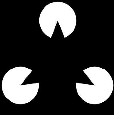
Figure 1: The Kanizsa triangle with curved boundaries. Notes the pop up of the illusory triangle out of the three pacman inducers.

A starting point to afford the task of modal completion is to consider illusory boundaries [37, 35, 20] and a number of mathematical models have been proposed on this topic. The celebrated model of elastica has been introduced by D.Mumford in [29] to take into account curvilinear illusory boundaries. Williams and Jacobs proposed a stochastic version of completion fields [42]. Recent models of boundary completion are based on the neurogeometrical structure of the visual cortex and they showed a strong explicative power of perceptual completion. The first neurogeometrical model has been introduced by Petitot and Y.Tondut [36] to describe the functional architecture of the visual cortex with instruments of differential geometry. In particular in [36] the hypercolumnar structure of the simple cells organization, responsible for contour detection, is modelled as a fiber bundle (see also section 2.2 below). The model has been further developed by Citti and Sarti [8], [38] who proposed to interpret the whole fiber bundle as the group of position and orientation with a subriemannian metric. This metric allows to reconstruct rectilinear or curved illusory boundaries. Other models of boundary completion have been developed in the same space [2, 4, 15, 34, 9, 10, 18, 42].

The problem of modal completion of both boundaries and figures together has been much less covered in literature. In [30] modal completion has been achieved by non-linear functional minimization by means of combinatorial techniques. In [39][40] it was proposed a technique to construct the Kanizsa triangle by minimization of an area functional measured with respect to a metric induced by the image. In both models [30] and [39] a complete boundary/figure reconstruction was provided but a correct filling in of figures with the perceived brighness is still missing.

In this paper we would like to introduce a formal field theory of low level vision, able to afford the problem of modal completion. The theory will couple two models of low level vision, i.e. a neurogeometrical model of boundary completion and the celebrated retinex algorithm as a model for filling in. In particular we will show that it is possible to integrate the retinex model of [13] with the neurogeometrical approach of [8] and to propose a new model of modal completion, based on complete contrast invariance. The two equations will act as a particle and a field term of a complete Gauge field theory.

The paper is organized as follows. In section 2 we recall the main properties of the Retinex algorithm and the neurogeometrical model, and reinterpret them with instruments of gauge field theory. In section 3 we couple the models by introducing a complete gauge field Lagrangian. The corresponding Euler Lagrange equations are calculated by variational calculus. In section 4 the Euler Lagrange equations are solved, providing results on the pop up of the Kanizsa figure. In Section 5 a plausible neural implementation of the model is proposed and discussed.

2 The retinex algorithm and the neurogeometrical model

In this section we recall the main properties of two previously recalled models retinex and the neurogeometrical one. The retinex algorithm has been inspired by the functionality of the retina in detecting image gradients and implementing contrast invariance. The second one has been inspired by the ability of the cortex to detect and complete boundaries. We will provide here a short description of the two processes, stressing the similarity of the mathematical instruments adopted by both.

2.1 A mathematical interpretation of the Retinex algorithm

The celebrated retinex model has been introduced in [24][23] to explain lightness perception, i.e. the phenomenon causing a gray patch to appear brighter when viewed against a dark background, and darker when viewed against a bright background. Here, we are more interested in his capacity of filling in figures from boundaries. After its introduction this model has inspired a wide range of improvements and new models have been proposed [7, 26, 25, 33, 19, 22].

In Horn’s work [17] the authors proposed a physically based algorithm, which recovers the reflectance $f$ of an image $I$ as

$$\Delta logf=\Delta logI.$$ (2.1)

In [27], it has been proved that the original Retinex algorithm can be equivalently espressed by the same equation. Precisely then Retinex is equivalent to a Neumann problem for a linear equation. The equation is identical to the Poisson equation for image editing proposed in Perez et al. [32]. In [13] a new interpretation was given in terms of covariant derivatives and fiber bundles. Indeed setting

$${\vec{A}}=\nabla I/I$$ (2.2)

equation 2.1 can be considered the Euler Lagrange equation of the functional

$$\tilde{F}=\int\frac{|\nabla f-{\vec{A}}f|^{2}}{f^{2}}dxdy.$$ (2.3)

This functional is invariant with respect to the transformation

$$f\to fI,\quad{\vec{A}}\to{\vec{A}}+\frac{\nabla I}{I}$$ (2.4)

so that the choice ${\vec{A}}=\frac{\nabla I}{I}$ is compatible with the transformations which leaves invariant the functional. The quantity $\nabla f-{\vec{A}}f$ can be interpreted as a covariant derivative.

Also note that, setting

$$\phi=logf,\quad h=logI,$$ (2.5)

equation 2.1 further simplify as

$$\Delta\phi=\Delta h$$ (2.6)

and with the same choice as before: ${\vec{A}}=\nabla I/I=\nabla g$ the functional becomes

$$F=\int|\nabla\phi-{\vec{A}}|^{2}dxdy=\int|\nabla\phi-\nabla h|^{2}dxdy,$$ (2.7)

while the transformations which leave invariant the operator become

$$\phi\to\phi+h,\quad{\vec{A}}\to{\vec{A}}+\nabla h.$$ (2.8)

2.2 A neurogeometrical model for boundary completion

Let us recall here the neurogeometrical model of boundary completion proposed by [8]. The model mimic the ability of simple cells of detecting boundaries and level lines of images, and to complete missing boundaries.

The retina can be modelled as a 2D plane, whose points will be denoted by $(x,y)$. Over each retinic point $(x,y)$ the primary visual cortex implements a whole fiber of cells, each one sensible to a specific direction $\theta$. Hence the set of simple cells is identified with the 3D space $R^{2}\times S^{1}$. A visual stimulus will be expressed as an image $I(x,y)$ defined on the retinal 2D plane, and we will denote $\bar{\theta}(x,y)$ the orientation of his level lines at every point. In presence of a visual stimulus, at every point $(x,y)$ the simple cell sensible to the orientation $\bar{\theta}(x,y)$ will be maximally activated. Hence the set of activated cells defines a surface in the 3D cortical space $R^{2}\times S^{1}$

$$\Sigma=\{(x,y,\theta):\theta=\bar{\theta}(x,y),|\nabla I(x,y)|>C\}.$$

The condition on the gradient of $I$ is a treshold, which ensures that the function $\bar{\theta}$ is well defined around boudaries of the image. If we set $\bar{H}(x,y,\theta)=\theta-\bar{\theta}(x,y)$, $\Sigma$ will be identified with the 0-level set of $\bar{H}$:

$$\Sigma=\{\bar{H}(x,y,\theta)=0,|\nabla I(x,y)|>C\}.$$

Simple cells are connected one to the other by the so called cortico-cortical connectivity. This connectivity is strongly anysotropic, and a cell located at a point $(x,y)$ and sensible to an orientation $\theta$ mainly propagate in the direction of its orientation $\theta$. More precisely the connectivity allows a propagation of the signal in the $R^{2}\times S^{1}$ along the integral curves of the vector fields

$$X_{1}=cos(\theta)\partial_{x}+\sin(\theta)\partial_{y},\quad X_{2}=\partial_{\theta}.$$ (2.9)

Propagation along the cortical connectivity seems to be at the basis of the process of boundary completion. Indeed the lifted surface $\Sigma$ is not defined on the whole space, but only over the region where boundaries or level lines are detected. The joint action of orientation detection and cortical propagation along the vector fields completes the surface extending it on the set $\{|\nabla I|<C\}$. In [8] it is shown that it can be expressed as the solution of the minimal surface equation

$$X_{1}\Big{(}\frac{X_{1}H}{\sqrt{|X_{1}H|^{2}+|X_{2}H|^{2}}}\Big{)}+X_{2}\Big{(}\frac{X_{2}H}{\sqrt{|X_{1}H|^{2}+|X_{2}H|^{2}}}\Big{)}=0,\text{ on }|\nabla I|<C$$ (2.10)

with internal boundary condition

$$H=\bar{H}\text{ on }|\nabla I|=C.$$

This last condition ensures that the existing boundaries are preserved, while the orientations of illusory boundaries or level lines are recovered as the 0 level set of the solution $H$.

This model performs completion of boundaries, giving rise to illusory contours, and of level lines, giving rise to amodal completion, as in the case of the macula cieca. But it is unable to perform filling when the level lines of the image are parallel to the missing or occluded regions, as in the case of modal completion of the Kanizsa triangle.

We explicitly note that this is a model of cortical 3D space of position and orientations. On the other hand the model defines a surface, that can be also expressed as a graph on the 2D space.

In facts, if we project the previous two vector fields on the $x,y$ plane, we end up with a unique derivative

$$X_{1\theta}=cos(\theta(x,y))\partial_{x}+\sin(\theta(x,y))\partial_{y}=<\nabla,(\cos(\theta(x,y)),\sin(\theta(x,y)))>$$ (2.11)

since the projection of the vector $X_{2}$ on the same plane is $0$. We explicitly note that the vector $X_{1\theta}$ here is only formally similar to the vector $X_{1}$ in (2.9). Indeed $\theta(x,y)$ in 2.11 is a function while in (2.9) $\theta$ was simply an axis of the 3D space.

The minimal surfaces equation can now be represented as the equation for a graph of $\theta(x,y)$, which is a function of the two variables $(x,y)$ alone. Hence the equation becomes:

$$X_{1\theta}\Big{(}\frac{X_{1\theta}\theta(x,y)}{\sqrt{|X_{1\theta}\theta(x,y)|^{2}+1}}\Big{)}=0,$$ (2.12)

where $\theta$ coincides with $\bar{\theta}$ on the existing boundaries. Taking explicitly the derivative, the equation is equivalent to

$$X_{1\theta}^{2}\theta(x,y)=0,$$ (2.13)

This equation can be interpreted as a second order directional derivative, in the direction $(\cos(\theta),\sin(\theta))$. Hence the norm, of the gradient coincides with the directional derivative:

$$|v|_{\theta}^{2}=\Big{(}<v,(\cos(\theta),\sin(\theta))>\Big{)}^{2}=\cos^{2}(\theta)v^{2}_{x}+\sin^{2}(\theta)v_{y}^{2}+2\cos(\theta)\sin(\theta)v_{x}v_{y}.$$ (2.14)

The projected norm of the gradient of $\theta$ reads:

$$|\nabla\theta|_{\theta}^{2}=|\cos(\theta)\partial_{x}\theta+\sin(\theta)\partial_{y}\theta|^{2}=$$

$$=\cos(\theta)^{2}|\partial_{x}\theta|^{2}+2\cos(\theta)\sin(\theta)\partial_{x}\theta\partial_{y}\theta+\sin(\theta)^{2}|\partial_{y}\theta|^{2}.$$

It’s easy to check that the second order equation (2.13) is simply the Euler Langrangian equation of the Dirichlet functional

$$\int|\nabla\theta(x,y)|_{\theta}^{2}dxdy.$$ (2.15)

Hence minima of this functional give rise to the same minimal graphs proposed in [8] for boundary propagation (see also [3] for a detailed proof).

3 The Gauge field model

3.1 The Lagrangian

We will provide a description of the low level vision process taking into account both the retinex model and the cortical neurogeometry. The task will be accomplished by considering the retinex model of Section 2.1 as the particle term and the cortical model of Section 2.2 as the field term of a classical gauge field theory.

In this way we will obtain an analogous of the classical theory of electromagnetism where both the particle and the fields are the unknown of the problem. Indeed, instead of equation (2.7) we propose a complete Lagrangian, sum of three terms: a particle term, an interaction term and a field term.

The particle term is

$$\mathcal{L}_{1}=\int|d\phi-dh|^{2}dxdy$$ (3.1)

and is directly inspired by the retinex model 2.7: it describes the reconstruction of the image from image boundaries. As described above it implements the perceptual invariance with respects to contrast. The next term describes the interaction beetween particle and field and it is again a retinex term acting not anymore on existing boundaries but on existing and illusory boundaries marked by the gauge field ${\vec{A}}$, that now is unknown:

$$\mathcal{L}_{2}=\int|d\phi-{\vec{A}}|^{2}dxdy.$$ (3.2)

It expresses the reconstruction of the image from the old and new boundaries explaining perceptual figure completion, by keeping contrast invariance properties. We explicitly note that in the minimization process ${\vec{A}}$ will have the direction of $\nabla\phi$, hence it will tend to be orthogonal to the existing boundaries or level lines. The orthogonality condition can be expressed in terms of directional derivatives in the direction of ${\vec{A}}$.

Finally the gauge field term will be analogous to the one of classical fields theories:

$$\tilde{{\mathcal{L}}}_{3}=\int|d{\vec{A}}|^{2}dxdy.$$ (3.3)

In our case it expresses the propagation of existing contours allowing the creation of subjective contours, and it will be modified accordingly to the the model presented in Section in 2.2, making use of the previously recalled subriemannian metric. In fact, propagation is expected in the direction of the boundary, which is orthogonal to ${\vec{A}}$: ${\vec{A}}^{\bot}=(-A_{y},A_{x})$. Since this vector is not unitary, we will normalize it to reduce to the norm defined in (2.14). The induced squared norm of $v$ reads:

$$|v|_{\vec{A}}^{2}=\Big{(}\frac{<v,{\vec{A}}>}{\sqrt{A_{x}^{2}+A_{y}^{2}}}\Big{)}^{2}=\frac{(-A_{y}v_{x}+A_{x}v_{y})^{2}}{A_{x}^{2}+A_{y}^{2}}=\frac{A_{y}^{2}v_{x}^{2}-2A_{x}A_{y}v_{x}v_{y}+A_{x}^{2}v_{y}^{2}}{A_{x}^{2}+A_{y}^{2}}.$$

Equivalently, if we call

$$G=(g^{ij})_{i,j=1,2}=\left(\begin{matrix}\frac{A_{y}^{2}}{A_{x}^{2}+A_{y}^{2}}&\frac{-A_{x}A_{y}}{A_{x}^{2}+A_{y}^{2}}\\ \frac{-A_{x}A_{y}}{A_{x}^{2}+A_{y}^{2}}&\frac{A_{x}^{2}}{A_{x}^{2}+A_{y}^{2}}\end{matrix}\right),$$ (3.4)

this norm can be computed as

$$|v|_{\vec{A}}^{2}=<Gv,v>,$$

hence the norm is formally the norm associated to the matrix $G=(g^{ij})$. In this setting $G$ is not invertile. On the contrary, in the riemannian setting, $G$ is invertible, and it has the role of the inverse of the metric of the space. When needed we will assume to introduce a small perturbation which makes its determinant non zero:

$$G_{\epsilon}=\left(\begin{matrix}\frac{A_{y}^{2}+\epsilon^{2}A_{x}^{2}}{A_{x}^{2}+A_{y}^{2}}&\frac{-A_{x}A_{y}(1-\epsilon^{2})}{A_{x}^{2}+A_{y}^{2}}\\ \frac{-A_{x}A_{y}(1-\epsilon^{2})}{A_{x}^{2}+A_{y}^{2}}&\frac{A_{x}^{2}+\epsilon^{2}A_{y}^{2}}{A_{x}^{2}+A_{y}^{2}}\end{matrix}\right).$$

We recall that the differential of ${\vec{A}}$ is independent of the norm chosen, and it is the usual curl operator:

$$d{\vec{A}}=curl({\vec{A}})=\partial_{x}A_{y}-\partial_{y}A_{x}.$$

The resulting functional $\mathcal{L}=\mathcal{L}_{1}+\mathcal{L}_{2}+\mathcal{L}_{3}$ is then

$$\mathcal{L}(h,\phi,{\vec{A}})=\int|d\phi-dh|^{2}dxdy+\int|d\phi-{\vec{A}}|^{2}dxdy+\int|d{\vec{A}}|_{{\vec{A}}}^{2}dxdy.$$ (3.5)

3.2 The Euler Lagrange equation

The Euler Lagrange Equation of the functional 3.5 becomes:

$$\Bigg{\{}\begin{matrix}\Delta\phi=\frac{1}{2}(\Delta h+div({\vec{A}}))\\ d_{\vec{A}}^{*}d{\vec{A}}=-\nabla_{\vec{A}}\phi+{\vec{A}}.\end{matrix}$$ (3.6)

These equations clearly have the meaning inherited by the corresponding terms of the functional: the first term is the particle equation that takes the two boundary terms (i.e. the rescaled Laplacian $\Delta g$ of the original image and the contribution $div({\vec{A}})$ generated by the gauge field ${\vec{A}}$ and performs a reconstruction of the image by filling in objects. Note that the two terms $\mathcal{L}_{1}$ and $\mathcal{L}_{2}$ which generalize the retinex functional give rise to an unique particle equation.

Note that ${\vec{A}}=(A_{x},A_{y})$ is a vector, hence the equation for ${\vec{A}}$ is indeed a system. In the same equation the directional gradient is defined as

$$\nabla_{\vec{A}}\phi=G\nabla\phi,$$

where $G$ is defined in (3.4).

The term $d_{\vec{A}}^{*}d$ coincides with $\nabla_{\vec{A}}^{\bot}\;curl({\vec{A}})$ (see Appendix A) and precisely:

$$d_{\vec{A}}^{*}d{\vec{A}}=\nabla_{\vec{A}}^{\bot}\;curl({\vec{A}})=-(\nabla_{\vec{A}}(\partial_{x}A_{y}-\partial_{y}A_{x}))_{y}dx+(\nabla_{\vec{A}}(\partial_{x}A_{y}-\partial_{y}A_{x}))_{x}dy.$$

(Here $A_{x}$ denotes the $x$ component of ${\vec{A}}$, not the derivative). In Appendix A we provide its explicit expression as sum of three terms:

$$d_{\vec{A}}^{*}d{\vec{A}}=\left\{\begin{matrix}\Delta_{{\vec{A}}}A_{x}-\partial_{x}a+T_{x}({\vec{A}})\\ \\ \Delta_{{\vec{A}}}A_{y}-\partial_{y}a+T_{y}({\vec{A}})\end{matrix}\right.$$

The terms $\Delta_{\vec{A}}$, $T_{x}({\vec{A}})$, $T_{y}({\vec{A}})$ are defined in (5.2). Precisely $\Delta_{\vec{A}}=div(\nabla_{\vec{A}})$ is the directional Laplacian associated to the considered metric. $T_{x}({\vec{A}}),T_{y}({\vec{A}})$ are advection terms, with coefficients depending on the metric, and

$$a=g^{12}\partial_{x}A_{y}+g^{22}\partial_{y}A_{y}+g^{11}\partial_{x}A_{x}+g^{12}\partial_{y}A_{x}.$$

The field equation on ${\vec{A}}$ propagates the gradient of the image, in the subriemmanian metric, and allows to recover existing and subjective boundaries. We explicitly note that the equation is of second order in the variable ${\vec{A}}$. In general functional of higher order are necessary to obtain completion of curved boundaries (as for example in the model of elastica [29]). However here the field ${\vec{A}}$ has the role of approximating the gradient of the image, following the lagrangian $L_{2}$, hence its second derivatives express third derivatives of the image function.

3.2.1 Nonlinearity of the equation

We remark that the differential equation for ${\vec{A}}$ is non linear, in the sense that the metric $G$ depends on ${\vec{A}}$ This means that we need to find an initial approximated solution ${\vec{A}}_{0}$. A natural choice is the solution of the vector Laplace equation

$$\Delta{\vec{A}}_{0}=\nabla\phi.$$

Of course this is only an approximated solution ${\vec{A}}_{0}$, but we can recover a better one ${\vec{A}}_{1}$ as a solution of

$$d_{{\vec{A}}_{0}}^{*}d{\vec{A}}_{1}=\nabla_{{\vec{A}}_{0}}\phi,$$

using the subriemmannian operator associated to ${\vec{A}}_{0}$. Recall that $\nabla_{{\vec{A}}_{0}}=G\nabla$. From here we start an iteration:

$$d_{{\vec{A}}_{1}}^{*}d{\vec{A}}_{2}=\nabla_{{\vec{A}}_{1}}\phi,\cdots\quad d_{{\vec{A}}_{j-1}}^{*}d{\vec{A}}_{j}=\nabla_{{\vec{A}}_{j-1}}\phi$$

At each step we get a better approximation of the solution, moreover the sequence has a limit ${\vec{A}}=\lim_{j\rightarrow+\infty}{\vec{A}}_{j}$. Passing to the limit in the previous expression, we will get:

$$d_{{\vec{A}}}^{*}d{\vec{A}}=\nabla_{{\vec{A}}}\phi,$$

so that the limit provides a solution of the nonlinear equation.

3.2.2 Invariance properties and choice of the gauge

The functional $\mathcal{L}$ is invariant with respect to the transformations:

$$h\to h^{\prime}=h+f,\;\;\phi\to\phi^{\prime}=\phi+f,\;\;{\vec{A}}\to{\vec{A}}^{\prime}={\vec{A}}+df$$

Indeed

$$d\phi^{\prime}-dh^{\prime}=d\phi-dh,\quad d\phi^{\prime}-A^{\prime}=d\phi-A,\quad d{\vec{A}}^{\prime}=d{\vec{A}}+ddf=d{\vec{A}}$$

since $d^{2}f=curldf=0$. This implies that the functional assumes the same values on $(h,\phi,{\vec{A}})$ and $(h^{\prime},\phi^{\prime},{\vec{A}}^{\prime})$

$$\mathcal{L}(h,\phi,{\vec{A}})=\mathcal{L}(h^{\prime},\phi^{\prime},{\vec{A}}^{\prime}).$$

Since the equation is invariant with respect to the choice of the gauge $f$, we can freely choose it, and the choice of the gauge will not affect the value of the Lagrangian. Hence we will make the choice which decouples and symplifies the system, imposing $a=0$. Since ${\vec{A}}={\vec{A}}^{\prime}-df,$ the expression of $a$ reduces to

$$a=g^{12}\partial_{x}(A^{\prime}_{y}-\partial_{y}f)+g^{22}\partial_{y}(A^{\prime}_{y}-\partial_{y}f)+g^{11}\partial_{x}(A^{\prime}_{x}-\partial_{x}f)+g^{12}\partial_{y}(A^{\prime}_{x}-\partial_{x}f),$$

where $f$ is an arbitrary choosen gauge function. To obtain $a=0$ we choose the function $f$ as a solution of

$$g^{22}\partial_{yy}f+g^{11}\partial_{xx}f+2g^{12}\partial_{yx}f=g^{12}\partial_{x}A^{\prime}_{y}+g^{22}\partial_{y}A^{\prime}_{y}+g^{11}\partial_{x}A^{\prime}_{x}+g^{12}\partial_{y}A^{\prime}_{x},$$

that is a second order subriemannian differential equation.

With this choice of the gauge, the second order term of the system reduces to the simpler form:

$$d_{\vec{A}}^{*}d{\vec{A}}=\left\{\begin{matrix}\Delta_{{\vec{A}}}A_{x}+T_{x}({\vec{A}})\\ \\ \Delta_{{\vec{A}}}A_{y}+T_{y}({\vec{A}})\end{matrix}\right.$$

where

$$\Delta_{{\vec{A}}}f=div(\nabla_{\vec{A}}f)=\frac{A_{y}^{2}\partial_{xx}f-2A_{x}A_{y}\partial_{xy}f+A_{x}^{2}\partial_{yy}f}{A_{x}^{2}+A_{y}^{2}}$$

$$T_{x}(\vec{A})=-\partial_{y}g^{11}\partial_{x}A_{x}-\partial_{y}g^{12}\partial_{y}A_{x}-\partial_{x}g^{21}\partial_{x}A_{y}-\partial_{x}g^{22}\partial_{y}A_{y}$$

$$T_{y}(\vec{A})=-\partial_{y}g^{12}\partial_{x}A_{y}-\partial_{y}g^{22}\partial_{y}A_{y}-\partial_{x}g^{11}\partial_{x}A_{x}-\partial_{x}g^{12}\partial_{y}A_{x}.$$

In conclusion we can rewrite the Euler Lagrange equation (3.6) in the form

$$\Bigg{\{}\begin{matrix}\Delta\phi=\frac{1}{2}(\Delta h+div({\vec{A}}))\\ \Delta_{{\vec{A}}}{\vec{A}}+T({\vec{A}})=-\nabla_{\vec{A}}\phi+{\vec{A}}.\end{matrix}$$ (3.7)

3.3 Solution of Euler Lagrange equations

The implementation of the algorithm consists in solving the system of coupled differential equation sequentially. We first apply the retinex equation to the initial image:

$$\Delta\phi=\frac{1}{2}\Delta h$$ (3.8)

and solve it by convolution

$$\phi=\frac{1}{2}\Big{(}\Gamma(x,y)*\Delta h\Big{)}$$

with the fundamental solution of the 2D Laplacian:

$$\Gamma(x,y)=log(|(x,y)|).$$

Then we solve the field equation for boundaries propagation. In this first phase we choose ${\vec{A}}=0$ in the right hand side, and the nonlinear equation reduces to

$$\Delta_{{\vec{A}}}{\vec{A}}+\vec{T}({\vec{A}})=\nabla\phi.$$

As we explained in the previous section, this equation will be solved by linearization, stopped after the first two steps:

$$\left\{\begin{matrix}\Delta{\vec{A}}_{0}=\nabla\phi\\ \Delta_{{\vec{A}}_{0}}{\vec{A}}_{1}+\vec{T}({\vec{A}})=\nabla\phi.\end{matrix}\right.$$ (3.9)

The solution of the first equation in (3.9) can be computed by convolution

$${\vec{A}}_{0}=\vec{\Gamma}*\nabla\phi,$$

where $\vec{\Gamma}(x,y)=(log(|(x,y)|),log(|(x,y)|))$ is the fundamental solution of the vector Laplacian. When applied to the Kanizsa inducers, the solution ${\vec{A}}_{0}$ is visualized in Figure 3, where the triangle inducers have been manually selected (Figure 2).

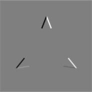
Figure 2: The $x$ and $y$ components of $\nabla h$ related to the Kanizsa triangle inducers.

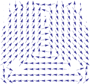
Figure 3: The normalized field ${\vec{A}}_{0}$ generated by the Kanizsa triangle inducers.

The second equation in the same system is a liner degenerate equation. If we approximate the matrix $G_{{\vec{A}}_{0}}$ with its riemannian approximation $\mathbb{G}_{\epsilon}$, it becomes elliptic. The solution of the linear elliptic differential equation

$$\Delta_{\epsilon{\vec{A}}_{0}}{\vec{A}}_{1}+\vec{T}({\vec{A}})=\nabla\phi$$

provides a good approximation of solution of the second equation in (3.9) and it can be obtained by finite differences methods (centered differences in space). The solution ${\vec{A}}_{1}$ is shown in Figure 4.

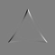
Figure 4: The x and y components of the gauge field ${\vec{A}}_{1}$ related to the Kanizsa triangle inducers. ${\vec{A}}_{1}$ is an approximation of the field ${\vec{A}}$, solution of the gauge field equation.

Since particle and field equations are coupled we can now solve the complete particle equation

$$\phi=\frac{1}{2}\Gamma(x,y)*\Big{(}\Delta h+\frac{1}{2}(div({\vec{A}}_{1})\Big{)}$$ (3.10)

again by convolution with the fundamental solution $\Gamma$. This is a version of the retinex equation able to reconstruct the original image together with the subjective surface. In Figure 5 left it is visualized the forcing term $\frac{1}{2}(\Delta h+div({\vec{A}}_{1}))$ of the particle equation while in Figure 5 right the solution $\phi$ is shown.

Figure 5: Left: The forcing term $\frac{1}{2}(\Delta h+div({\vec{A}}_{1}))$ of the particle equation. Right: The reconstructed Kanizsa triangle as the solution $\phi$ of the particle equation.

3.4 A neural implementation in LGN and Cortex

In order to further support our model, we will discuss how the different terms of the Lagrangian can be implemented in neurophysiological structures.

We recall that the visual signal is first elaborated by the retina whose receptive profiles are well modeled by the classical Laplacian of Gaussian:

$$\Delta{\it G}_{\sigma}=\Delta e^{\frac{-x^{2}}{2\sigma^{2}}},$$

where $\Delta$ is the standard Laplacian. We can observe that the same receptive profiles are found in the Lateral Geniculate Nucleus (LGN), that is a copy of the retina but stricly in contact with the visual cortex. The action of these receptive fields on the visual signal can be represented as the output of the neural cell

$$\Delta{\it G}_{\sigma}*\log I=\Delta h$$

where $g$ is a smoothed version of the $\log I$ and the logarithmic function is due to the non linearity of the cell response. The output of LGN cells is propagated via the horizontal connectivity in LGN. Since this connectivity is isotropic, it can be modeled with the fundamental solution $\Gamma(x,y)$ of the 2D Laplacian operator. LGN horizontal connectivity with strength $\Gamma(x,y)$ acts linearly on the feedforward input $h$, giving a total contribution

$$\phi=\frac{1}{2}\Big{(}\Gamma*\Delta h\Big{)}.$$

This is exactly the solution of the Laplacian equation (3.8) of the particle term, implementing the reconstruction of the image from the boundaries. Note that the action of receptive profiles $\Delta h(x,y)$ and the one of LGN horizontal connectivity $\Gamma(x,y)*$ is dual in a differential sense.

The gauge field equation in ${\vec{A}}$ performs boundaries propagation and we will conjecture now how it is implemented at the cortical level. Simple cells performs stimulus differentiation $\nabla\phi$ that is propagated by horizontal connectivity in the direction of the stimulus orientation[6, 1]. For this reason horizontal connectivity can be modelled by the fundamental solution of the vector Laplacian $\vec{\Gamma}(x,y)$ and the total connectivity excited by the stimulus can be accounted as

$${\vec{A}}_{0}=\vec{\Gamma}*\nabla\phi.$$

Now, the feedforward output of simple cells $\nabla\phi$ is propagated by the excited connectivity ${\vec{A}}_{0}$ generating the distribution ${\vec{A}}_{1}$, solution of:

$$\Delta_{{\vec{A}}_{0}}{\vec{A}}_{1}+\vec{T}({\vec{A}})=\nabla\phi.$$

We have shown in [8] that ${\vec{A}}_{1}$ is the field tangent to the perceptual association fields measured by Fields, Hayes and Hess in [12] and it is cortically implemented by means of horizontal connectivity propagation.

Finally, the forcing term ${\vec{A}}$ in the particle equation can be interpreted as the feedback of the cortical processing to LGN, showing the strength of the gauge field theory in coupling the activity of different physiological layers. Equation (3.10) is again the retinex equation, but with the feedback from V1 that takes into account illusory boundaries.

4 Conclusions

In this paper we made the effort to construct a formal field theory of low level vision. Contemporary instruments of field theory based on Gauge invariances have been used to introduce a complete Lagrangian with its particle, interaction and field terms. The Lagrangian couples two well known models for lightness and boundary propagation, i.e. the retinex and the neurogeometrical models. Particularly the problem of modal completion of illusory figures is faced and it is shown how the Euler-Lagrange field equations well represent the process of constitution of the Kanizsa triangle with curved boundaries. But the interest of the model overcome the formal analogy with particle-fields physical theory. In facts it has to be considered as a plausible model for the interaction between different structures of the visual systems, particularly regarding the coupling between the activity of LGN and the one of the visual cortex. The Gauge Lagrangian formulation seems to be strongly enough to describe both the feedforward and the feedback processes of low level vision, by keeping the desired invariances.

5 Appendix

We rapidly recall here the definition of differential in the riemannian setting, in the special case where det $G$ is a constant, which is the case of the metric in LABEL:. We will call $G=g^{-1}$ since $G$ plays the role of inverse of the metric. Then the riemannian scalar product is defined as:

$$<v,w>_{g}=<gv,w>.$$

If $a$ is a function then we will denote $da$ the usual differential, whose components are $\nabla a=(\partial_{x}a,\partial_{y}a)$

$$da=\partial_{x}adx+\partial_{y}ady.$$

The gradient of the function $a$ in the metric $g$ is defined as

$$\quad\nabla_{g}a=G\nabla a=\left(\begin{matrix}g^{11}&g^{12}\\ g^{21}&g^{22}\end{matrix}\right)\left(\begin{matrix}\partial_{x}a\\ \partial_{y}a\end{matrix}\right)$$

In the sequel we will denote $((\nabla_{g}a)_{x},(\nabla_{g}a)_{y})$ its components. The laplacian is expressed as

$$\Delta_{g}a=div(\nabla_{g}a).$$

If ${\vec{A}}=A_{x}dx+A_{y}dy$, then

$$d{\vec{A}}=curl({\vec{A}})=(\partial_{x}A_{y}-\partial_{y}A_{x})\;\;dx\wedge dy$$

and the Laplacian is not the laplacian of the two components in general, but can be expressed in terms of the $d$ and $d^{*}$ operators, which we will now define. Since $d{\vec{A}}$ is a 2-form, first recall that for a general 2-form $\beta=bdx\wedge dy$

$$d^{*}\beta=-(\nabla_{g}b)_{y}dx+(\nabla_{g}b)_{x}dy$$

$$=-(g^{21}\partial_{x}b+g^{22}\partial_{y}b)dx+(g^{11}\partial_{x}b+g^{12}\partial_{y}b)dy$$

(formally its components are $\nabla_{g}^{\bot}b$, so that so that, while applying to $d\alpha$,

$$d^{*}d{\vec{A}}=\nabla_{g}^{\bot}curl(\alpha)=-(\nabla_{g}(\partial_{x}A_{y}-\partial_{y}A_{x}))_{y}dx+(\nabla_{g}(\partial_{x}A_{y}-\partial_{y}A_{x}))_{x}dy.$$ (5.1)

The vanishig condition of this expression (which will be used in section ??) is a system in two variables.

$$\left\{\begin{matrix}(\nabla_{g}\partial_{y}A_{x})_{y}-(\nabla_{g}\partial_{x}A_{y})_{y}=0\\ \\ (\nabla_{g}\partial_{x}A_{y})_{x}-(\nabla_{g}\partial_{y}A_{x})_{x}=0\end{matrix}\right.$$

We can now exchange the order of differentiation: we call $[\nabla_{g},\partial_{x}]=\nabla_{g}\partial_{x}-\partial_{x}\nabla_{g}$

$$\left\{\begin{matrix}\partial_{y}(\nabla_{g}A_{x})_{y}+[\partial_{y},(\nabla_{g})_{y}]A_{x}-\partial_{x}(\nabla_{g}A_{y})_{y}-[\partial_{x},(\nabla_{g})_{y}]A_{y}=0\\ \\ \partial_{x}(\nabla_{g}A_{y})_{x}+[\partial_{x},(\nabla_{g})_{x}]A_{y}-\partial_{y}(\nabla_{g}A_{x})_{x}-[\partial_{y},(\nabla_{g})_{x}]A_{x}=0\end{matrix}\right.$$

Now we note that $div((\nabla_{g}A_{x})=\partial_{x}(\nabla_{g}A_{x})_{x}+\partial_{y}(\nabla_{g}A_{x})_{y}$

$$\left\{\begin{matrix}div(\nabla_{g}A_{x})+[\partial_{y},(\nabla_{g})_{y}]A_{x}-[\partial_{x},(\nabla_{g})_{y}]A_{y}-\partial_{x}((\nabla_{g}A_{x})_{x}+(\nabla_{g}A_{y})_{y})=0\\ \\ div(\nabla_{g}A_{y})+[\partial_{x},(\nabla_{g})_{x}]A_{y}-[\partial_{y},(\nabla_{g})_{x}]A_{x}-\partial_{y}((\nabla_{g}A_{x})_{x}+\nabla_{g}A_{y})_{y})=0\end{matrix}\right.$$

Now we give a name of each term in this expression,

$$\left\{\begin{matrix}div(\nabla_{g}A_{i})=\Delta_{g}A_{i}\quad\quad\quad\quad\quad\quad\quad\quad\quad\quad\quad\quad\quad\quad\quad\quad\quad\quad\quad\quad\quad\quad\quad\\ T_{x}(\vec{A})=[\partial_{y},(\nabla_{g})_{y}]A_{x}-[\partial_{x},(\nabla_{g})_{y}]A_{y}=\quad\quad\quad\quad\quad\quad\quad\quad\quad\quad\quad\quad\quad\\ \quad\quad\quad\quad\quad\quad\quad\quad=-\partial_{y}g^{11}\partial_{x}A_{x}-\partial_{y}g^{12}\partial_{y}A_{x}-\partial_{x}g^{21}\partial_{x}A_{y}-\partial_{x}g^{22}\partial_{y}A_{y}\\ T_{y}(\vec{A})=[\partial_{x},(\nabla_{g})_{x}]A_{y}-[\partial_{y},(\nabla_{g})_{x}]A_{x}=\quad\quad\quad\quad\quad\quad\quad\quad\quad\quad\quad\quad\quad\\ \quad\quad\quad\quad\quad\quad\quad\quad=-\partial_{y}g^{12}\partial_{x}A_{y}-\partial_{y}g^{22}\partial_{y}A_{y}-\partial_{x}g^{11}\partial_{x}A_{x}-\partial_{x}g^{12}\partial_{y}A_{x}\\ a=(\nabla_{g}A_{x})_{x}+(\nabla_{g}A_{y})_{y}=g^{12}\partial_{x}A_{y}+g^{22}\partial_{y}A_{y}+g^{11}\partial_{x}A_{x}+g^{12}\partial_{y}A_{x}\end{matrix}\right.$$ (5.2)

Finally we conclude that the first variation of the functional

$$\int|d{\vec{A}}|_{\vec{A}}^{2}$$

can be expressed as

$$d^{*}d{\vec{A}}=\nabla_{g}^{\bot}curl({\vec{A}})=\left\{\begin{matrix}\Delta_{g}A_{x}-\partial_{x}a+T_{x}({\vec{A}})\\ \\ \Delta_{g}A_{y}-\partial_{y}a+T_{y}({\vec{A}})\end{matrix}\right.$$

References

- [1] Angelucci, A., Levitt, J.B., Walton, E.J.S., Hupe, J., Bullier, J., Lund, J.S.: Circuits for local and global signal integration in primary visual cortex. J. Neurosci. 22(19), 8633-46 (2002)
- [2] J. August, S. Zucker, Sketches with curvature: The curve indicator random field and markov processes, IEEE Trans. Pattern Anal. Mach. Intell, 25(4), 387-400, 2003.
- [3] D. Barbieri, G.Citti, Regularity of minimal intrinsic graphs in 3 dimensional sub-Riemannian structures of step 2, Journal des Mathématiques Pures et Appliquées, 96(3), 279-306, 2011.
- [4] O. Ben-Shahar, S.W. Zucker, Geometrical Computations Explain Projection Patterns of Long Range Horizontal Connections in Visual Cortex, Neural Computation, 16 (3), 445- 476, 2004.
- [5] M. Bertalmio, G. Sapiro, V. Castelles, C. Ballester, Image Inpainting, Proceedings of ACM SIGGRAPH, ACM Press, 417-424, 2000.
- [6] Bosking, W.H., Zhang, Y., Schofield, B., Fitzpatrick, D.: Orientation selectivity and the arrangement of horizontal connections in tree shrew striate cortex. J. Neurosci. 17(6), 2112-27 (1997)
- [7] D. H. Brainard, B. A. Wandell, Analysis of the retinex theory of color vision, J. Opt. Soc. Amer. A, 3 (10), 1651, 1986.
- [8] G. Citti, A. Sarti, A Cortical Based Model of Perceptual Completion in the Roto-Translation Space, J. Math. Imaging and Vision, 24 (3), 307-326, 2006.
- [9] R. Duits and E. M. Franken, Left invariant parabolic evolution equations on SE(2) and contour enhancement via invertible orientation scores, part I: Linear left-invariant diffusion equations on SE(2), Quarterly of Applied mathematics, AMS, 68, 255-292, 2010.
- [10] R. Duits and E. Franken, Left invariant parabolic evolution equations on SE(2) and contour enhancement via invertible orientation scores, part II: Nonlinear left-invariant diffusion equations oninvertible orientation scores,” Quarterly of Applied mathematics, AMS, 68, 293-331, 2010.
- [11] D. Field, A. Hayes, Contour integration and lateral connections of v1 neurons. In LM Chalupa and JS Werner (Eds.), The visual neurosciences, 2, 1069-1079, 2004.
- [12] Field, D.J., Hayes, A., Hess, R.F.: Contour integration by the human visual system: evidence for a local association field. Vision Res. 33, 173-193 (1993)
- [13] T. Georgiev, Covariant derivatives and vision Lecture Notes in Computer Science (including subseries Lecture Notes in Artificial Intelligence and Lecture Notes in Bioinformatics) 3954 LNCS, 56-69, 2006.
- [14] T. Georgiev, Vision, healing brush, and fibre bundles Proceedings of SPIE - The International Society for Optical Engineering 5666, 33, 293-305, 2005.
- [15] G. Ben-Yosef, O. Ben-Shahar, A Tangent Bundle Theory for Visual Curve Completion, IEEE Transactions on Pattern Analysis and Machine Intelligence, 34 (7), 2012.
- [16] W. Hoffman. Higher visual perception as prolongation of the basic lie transformation group. Mathematical Biosciences, 6, 437 -471, 1970.
- [17] B. K. P. Horn, Determining lightness from an image, Comput. Graph. Image Process., 277-299, 1974.
- [18] R.K. Hladky and S.D. Pauls, “Minimal Surfaces in the Rototranslational Group with Applications to a Neuro-Biological Image Completion Model,” J. Math. Imaging and Vision, 36, 1-27, 2010.
- [19] A. Hurlbert, “Formal connections between lightness algorithms,” J. Opt. Soc. Amer. A, 3 (10), 1684, 1986.
- [20] G. Kanizsa, Organization in vision. New York: Praeger, 1979.
- [21] P. J. Kellman, T. F. Shipley, A theory of visual interpolation in object perception. Cognitive Psychology, 23, 141-221,1991.
- [22] R. KimmelL, M. Elad, D. Shaked, R. Keshet, I. Sobel, A Variational Framework for Retinex, International Journal of Computer Vision, 52 (1), 7–23, 2003.
- [23] E. H. Land, The retinex theory of color vision, Scientific American, 237 (6), pp. 108-128, 1977.
- [24] E. Land, J. McCann, Lightness and retinex theory, J. Opt. Soc. Amer., 61 (1), 1–11, 1971.
- [25] L. Lei, Y. Zhou, J. Li, An investigation of retinex algorithms for image enhancement, J. Electron., 24 (5), 696-700, 2007.
- [26] J. M. McCann et al., Retinex at 40: A joint special session, J. Electron.Imag., 13, 6, 2002.
- [27] J-M Morel A PDE Formalization of Retinex Theory, IEEE Transactions on image processing, 19 (11), 2010.
- [28] S. Masnou, J-M Morel, Level lines based disocclusion IEEE International Conference on Image Processing 3, 259-263, 1998.
- [29] D. Mumford, Elastica and computer vision. In Algebraic Geometry and Its Applications, Chandrajit Bajaj (Ed.). Springer- Verlag: New York, 1994.
- [30] M.Nitzberg, D.Mumford, T.Shiota, Filtering, Segmentation and Depth, Lecture Notes in Computer Science, Springer-Verlag, Berlin-Heidelberg 1993
- [31] R. Palma-Amestoy, E. Provenzi, M. Bertalmio, and V. Caselles, A perceptually inspired variational framework for color enhancement, IEEE Transactions on Pattern Analysis and Machine Intelligence, 31 (3), 458-474, 2009.
- [32] P. Perez, M. Gangnet, and A. Blake, Poisson image editing, ACM Trans. Graph., 22 (3), 313-318, 2007.
- [33] E. Provenzi, L. D. Carli, A. Rizzi, and D. Marini, “Mathematical definition and analysis of the retinex algorithm,” J. Opt. Soc. Amer. A, 2, 2613 - 2621, 2005.
- [34] X. Ren, C. Fowlkes, J. Malik, Learning Probabilistic Models for Contour Completion in Natural Images, Int’l J. Computer Vision, 77 (1-3), 47-63, 2008.
- [35] D. Ringach, R. Shapley, Spatial and Temporal Properties of Illusory Contours and Amodal Boundary Completion, Vision Research, 36 (19), 3037 - 3050, 1996.
- [36] J. Petitot, The neurogeometry of pinwheels as a sub-Riemannian contact structure. Journal of Physiology - Paris 97, 265-309, 2003.
- [37] S.E. Petry, G.E. Meyer The perception of illusory contours. Springer, 1987.
- [38] A. Sarti, G. Citti, J. Petitot, The symplectic structure of the primary visual cortexv Biological Cybernetics, 98 (1), 33-48, 2008.
- [39] A. Sarti, R. Malladi, J.A. Sethian, Subjective surfaces: A geometric model for boundary completion, International Journal of Computer Vision, 46 (3), 201-221, 2002.
- [40] A. Sarti, R. Malladi, J.A. Sethian, Subjective surfaces: A method for completing missing boundaries, Proceedings of the National Academy of Sciences of the United States of America, 97 (12) , 6258-6263, 2000.
- [41] Michael Wertheimer, A Brief History of Psychology. Harcourt Brace, 2000.
- [42] L.R. Williams, D.W. Jacobs, “Stochastic Completion Fields: A Neural Model of Illusory Contour Shape and Salience, Neural Computation, 9 (4), 837-858, 1997.