X-ray transition yields of low-$Z$ kaonic atoms produced in Kapton

Abstract

The X-ray transition yields of kaonic atoms produced in Kapton polyimide ($\rm{C}_{22}\rm{H}_{10}\rm{N}_{2}\rm{O}_{5}$) were measured for the first time in the SIDDHARTA experiment. X-ray yields of the kaonic atoms with low atomic numbers ($Z=6,7,$ and 8) and transitions with high principal quantum numbers ($n=5-8$) were determined. The relative yields of the successive transitions in the same atoms and the yield ratios of carbon-to-nitrogen (C:N) and carbon-to-oxygen (C:O) for the same transitions were also determined. These X-ray yields provide important information for understanding the capture ratios and cascade mechanisms of kaonic atoms produced in a compound material, such as Kapton.

1 Introduction

The study of kaonic atoms provides unique information on low-energy QCD in the strangeness sector. The energy shifts and widths of the lowest-lying levels permit extraction of the strong interaction in the low-energy regime. See, for example, the recent experimental results [1, 2, 3, 4], and references therein. The upper-level widths caused by the strong interaction can be determined using the relative yields of the lowest-lying levels and the levels feeding it. These widths have been used for theoretical calculations of the kaon-nucleon/nucleus interaction (e.g., [5, 6, 7, 8]).

On the other hand, even if higher X-ray transitions are not significantly affected by the strong interaction between the kaon and nucleus, the X-ray yields provide fundamental information on the atomic capture, initial distribution and de-excitation processes.

Cascade calculations based on kaonic atom X-ray yields taken with several solid targets [9, 10] were initially performed using the Fermi-Teller model [11]. The results showed a smooth variation of the yields over atomic number $Z$, as shown in Fig. 2 of Ref. [11].

When this data set was extended to targets ranging from helium ($Z=2$) through uranium ($Z=92$) [12], a striking result was obtained. Unlike the earlier prediction of Ref. [11], an unexpected variation in the pattern of X-ray yields vs atomic number was observed. This variation has several maxima and minima, as shown in Fig. 7 of Ref. [12], where the maxima occur near the closed atomic electron shells.

Similar yield patterns were observed in muonic and pionic atom X-ray yields, as well as positron-annihilation lifetimes in annealed metals [13]. Theoretical studies showed that these patterns could be related to the properties of the exotic atoms, such as the atomic radii, the initial distributions of the particles, etc. [13, 14].

Although a large amount of data on kaonic atom X-ray yields was collected, transitions with a high principal number $n$ in materials of low atomic number $Z$ have not previously been measured due to the low energy of the X-rays in such transitions. It is of interest to explore such unmeasured regions both experimentally and theoretically.

Previous yield measurements were mainly of pure solid materials. However, X-ray yields in compounds such as hydrides (LiH, CH, NaH, and CaH₂) were reported to have reductions of 20-70% [15, 16], possibly related to the Stark effect of the protons in the hydrides and the kaon transfers.

In this paper, we report on the first determination of the X-ray yields of kaonic atoms produced in the Kapton polyimide ($\rm{C}_{22}\rm{H}_{10}\rm{N}_{2}\rm{O}_{5}$) foils, which were used as a target window material in the SIDDHARTA experiment.

2 The SIDDHARTA experiment

The SIDDHARTA experiment was performed using low-energy kaons produced by the DA$\Phi$NE electron-positron collider. The main purpose of the experiment was the measurement of X-rays from kaonic atoms formed in gaseous targets. In addition, we measured kaonic atom X-rays produced in the windows of the gaseous target cell. These latter X-ray yields are reported in this paper.

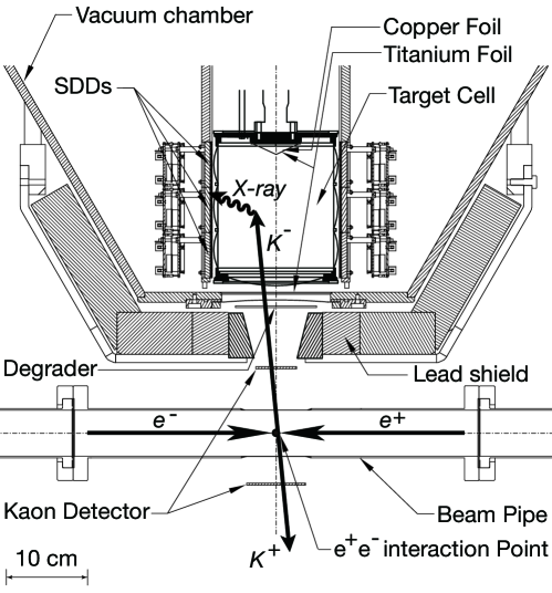
Figure 1: A schematic view of the SIDDHARTA setup installed at the e⁺e^- interaction region of DA$\rm{\Phi}$NE.

Figure 1 shows the schematic view of the experimental setup. Electrons and positrons collided at the DA$\Phi$NE interaction point, where almost at-rest $\phi$ mesons were created. $K^{+}K^{-}$ pairs produced by $\phi$ decay were emitted from the interaction point. The $K^{+}K^{-}$ pairs were detected by a kaon detector consisting of two plastic scintillators placed above and below the interaction point. The timing signals of the $K^{+}K^{-}$ pairs were recorded using clock signals with a frequency of 120 MHz. Because of a finite crossing angle of the electron and position beams, the momentum of the emitted kaons had an angular dependence. This angular dependence was compensated using a stepped degrader made of Mylar foils with thicknesses ranging from 100 to 800 $\mu$m. The thicknesses of the degrader were optimized to increase kaon stops in the target gas.

The charged kaons entered the target cell after passing through the scintillator and degrader. The cylindrical target cell, made of Kapton polyimide ($\rm{C}_{22}\rm{H}_{10}\rm{N}_{2}\rm{O}_{5}$) foils with a thickness of 75 microns and a density of 1.42 g/cm³, was 15.5 cm high with a diameter of 13.7 cm. The bottom of the target cell, through which the charged kaons entered, was also made of Kapton. On the top of the target cell, thin Ti and Cu foils were installed to produce fluorescence X-rays induced by the beam background.

In the experiment, we used four target gases: hydrogen (1.30 g/$l$), deuterium (2.50 g/$l$), helium-3 (0.96 g/$l$) and helium-4 (1.65 g/$l$ and 2.15 g/$l$). They were cooled to 23 K. The charged kaons stopped mainly in the target gas and partially in the Kapton windows. The number of kaons stopping in the target gas and the windows, which depends on the target density, was determined by Monte Carlo simulations.

Figure 2: A picture of the target cell made of Kapton and the SDDs together with the readout electronics.

The X-rays were measured by silicon drift detectors (SDDs), which surrounded the target as shown in Fig. 2. Each SDD has an effective area of 1 cm² with a 450-$\mu$m thickness. There were 144 SDDs in total. The SDDs were cooled to a temperature of 170 K to obtain an excellent energy resolution of about 150 eV for 6 keV X-rays, which is close to the resolution in noise-free conditions.

The data on the kaonic atom X-rays were accumulated in 2009. The X-ray yields of the kaonic atoms produced in the Kapton windows were determined using the data taken with deuterium gas (an integral luminosity of 92 pb^-1). In these data, since kaonic deuterium X-ray peaks were very small [17], X-ray peaks from Kapton can be easily extracted. In contrast, the data taken with other gases were not suitable due to overlapping peaks.

3 Data analysis

The data taken with the SDDs and the kaon detector were analyzed to extract kaonic atom X-ray spectra. The analysis methods given in Refs. [3, 4] were used in the following procedures with the addition of a method dedicated to determination of the X-ray yields.

The energy scales were calibrated for each SDD, where the data taken with the Ti and Cu foils excited by an X-ray tube and the beam background were used [1, 2, 3, 4, 17]. A typical energy spectrum of the data taken with one SDD is shown in Fig. 3. High statistics of the fluorescence Ti and Cu X-rays were obtained. Since the X-ray energies of these lines are well known [18, 19], the energy scale was calibrated using the peak positions of the K$\alpha$ lines, assuming good integral linearity of the analogue-to-digital converters (ADCs). The Ti and Cu K$\beta$ lines are not suitable for a detailed energy calibration due to the existence of satellite transitions close to the K$\beta$ lines [20, 21, 22]. In addition to the energy calibration, the time dependent instability was corrected for each SDD. The energy calibration and the instability correction were performed every few hours. Among the 144 SDDs, 94 were selected for further analysis based on energy resolution, stability, and peak shapes.

Figure 4 shows the energy spectrum obtained with 94 SDDs with timing uncorrelated to the $K^{+}K^{-}$ pairs. Together with the large beam background, there are fluorescence X-ray peaks at 4.5, 8.0, and 9.6 keV, which were identified as the Ti K$\alpha$, Cu K$\alpha$ and Au L$\alpha$ lines. The Ti and Cu lines were produced in the foils installed on the top of the target cell, while the Au line was produced in the material of the printed-circuit boards of the SDDs.

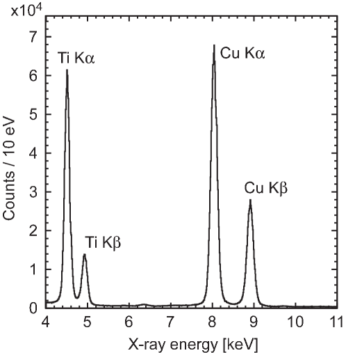
Figure 3: A typical energy spectrum for one SDD in the calibration data with the X-ray tube irradiating the Ti and Cu foils. The energy scale was calibrated using the positions of the Ti and Cu K$\alpha$ lines.

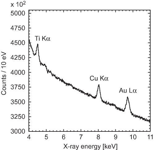
Figure 4: Energy spectrum for the selected 94 SDDs, where the timing uncorrelated to the $K^{+}K^{-}$ pair productions was selected. The accuracy of the energy scale was evaluated using the peak positions of the Ti K$\alpha$, Cu K$\alpha$, and Au L$\alpha$ lines.

The accuracy of the energy scale determined was examined using these peak positions. The fit of the X-ray peaks showed that the gain was slightly shifted by about 6 eV. The gain shift was expected because the hit rates of the SDDs were much higher in the calibration data. This gain shift was corrected. The accuracy of the energy scale was found to be $\pm 4$ eV, which was determined using the difference between the known X-ray energies and the peak positions after the gain correction [3, 4].

High radiation caused by the large beam loss introduces a latch-up phenomenon in some of the SDDs. The latch-up was automatically recovered by re-applying the voltages on the SDDs. However, the SDDs could not measure in the periods of the latch-up. The evaluation of X-ray event loss caused by the latch-up (i.e. dead time correction) is not simple, because it depends not only on the number of latched-up SDDs, but also on the beam conditions, etc. To dismiss the dead time correction, we selected only the periods of data taking without any latched-up SDDs. About 20% of the total data were rejected by this selection.

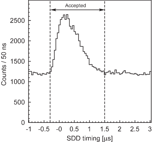
Figure 5: Timing spectrum of SDDs. The time difference between the $K^{+}K^{-}$ coincidence and SDD X-ray hits is plotted. The peak region corresponds to the coincidence of the $K^{+}K^{-}$ and X-ray events. The region indicated by arrows was selected as the good timing of the X-ray events.

The time differences between the coincidences in the kaon detector and the X-ray hits in the SDDs were also measured. Figure 5 shows the spectrum of the time difference, where the time walk effect was corrected using the correlation between the X-ray energy and timing. The origin of the time scale is arbitrary. The continuous flat background seen in the figure corresponds to the beam background uncorrelated to the kaon timing. The events correlated to the kaon timing are seen as the peak. The broadening of the peak corresponds to the drift time of the charges generated by the X-rays in the SDDs. The peak area corresponds to kaonic atom X-ray events together with the beam background correlated to the kaon timing (e.g., secondary particles produced by kaon decay and nuclear reactions). For the X-ray energy spectra, event selection using timing suppresses the background uncorrelated with the kaon timing. The timing region was selected as indicated by the arrows in the figure, where the X-ray event loss caused by this selection was determined to be less than 1%.

The $K^{+}K^{-}$ pairs produced by $\phi$ decay were detected by the kaon detector. The charged kaons were identified by a time-of-flight technique, using the beam timing signals delivered by DA$\Phi$NE. The time differences between the beam timing signals and the coincidences in the kaon detector were measured. Figure 6 shows a correlation of the time differences measured in the two scintillators of the kaon detector. The origin of the timing is arbitrary. The events corresponding to the $K^{+}K^{-}$ pairs were marked in the figure. In addition to the $K^{+}K^{-}$ pairs, fast minimum-ionizing particles (MIPs), generated by the beam background, also passed through the two scintillators in coincidence, as shown in Fig. 6. These $K^{+}K^{-}$ pairs and MIPs appear in two regions because the half frequency of the beam timing signals was used. The regions marked with a rectangle were accepted as the timing windows for the $K^{+}K^{-}$ coincidence. The number of $K^{+}K^{-}$ events was determined to be

$$N_{trig}^{EXP}=8.495\cdot 10^{6}.$$ (1)

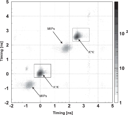
Figure 6: Timing spectrum of the kaon detector. The correlation of the time differences measured in the two scintillators is shown. The coincidence events of $K^{+}K^{-}$’s and MIPs were marked in the figure. The regions with a rectangle were accepted as the timing windows of the $K^{+}K^{-}$ coincidence.

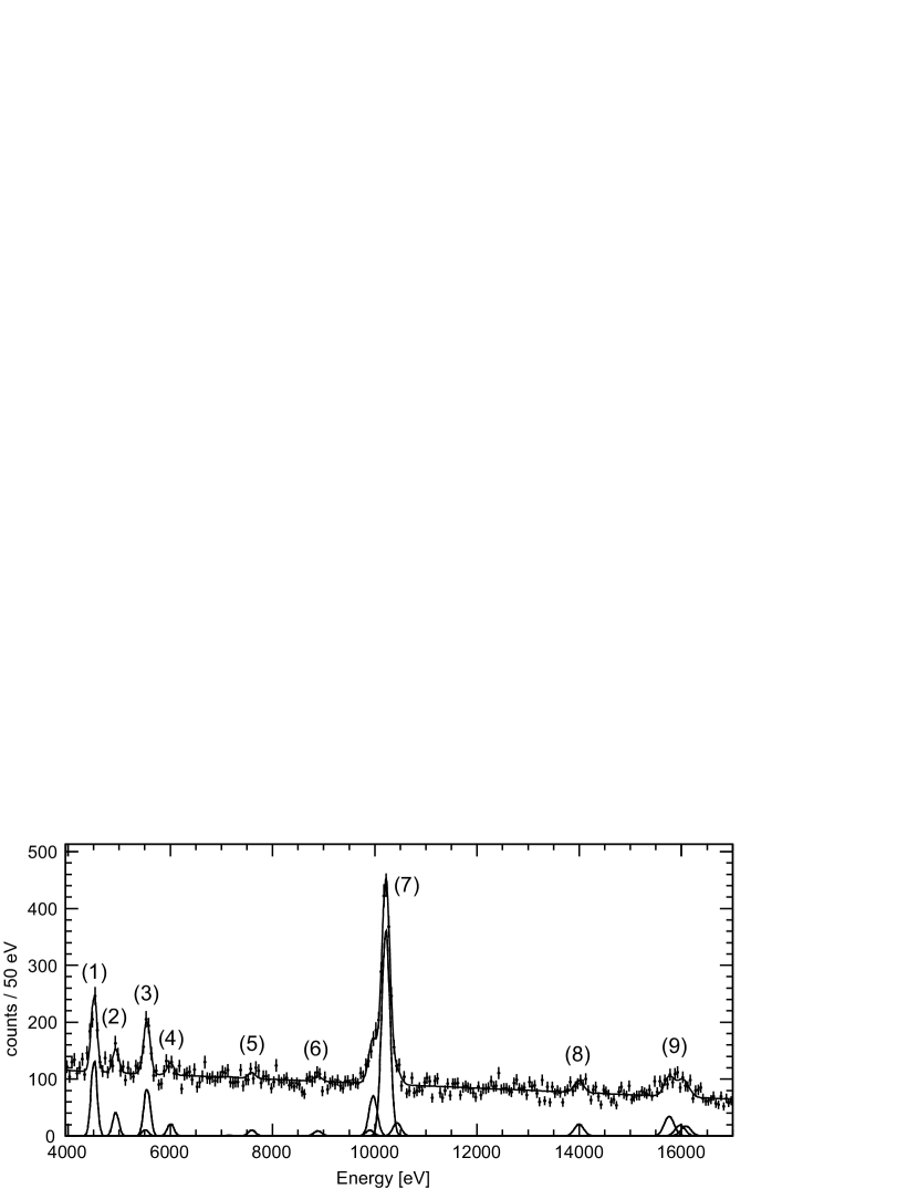
Figure 7: Energy spectrum of the kaonic atom X-rays produced in Kapton, where the target cell was filled with deuterium. (1) Ti K$\alpha$, (2) Ti K$\beta$, (3) kaonic carbon ($K^{-}$C) $8\to 6$ and $6\to 5$, (4) kaonic oxygen ($K^{-}$O) $7\to 6$, (5) kaonic nitrogen ($K^{-}$N) $6\to 5$, (6)$K^{-}$N $7\to 5$, (7)$K^{-}$O $8\to 6$ and $6\to 5$, $K^{-}$C $5\to 4$, and kaonic aluminum ($K^{-}$Al) $8\to 7$, (8)$K^{-}$N $5\to 4$, and (9) $K^{-}$C $6\to 4$, $K^{-}$O $7\to 5$, and $K^{-}$Al $7\to 6$ transitions.

With timing cuts on the SDDs and event selection on the $K^{+}K^{-}$ pairs in the kaon detector, a clean energy spectrum of the kaonic atom X-rays was extracted. Figure 7 shows the energy spectrum from the deuterium gas target, where the number of SDDs used in the analysis is

$$N^{EXP}_{SDD}=94.$$ (2)

The peaks shown in the figure were attributed to X-ray transitions in the kaonic atoms formed in Kapton. Since Kapton contains carbon, nitrogen, oxygen, and hydrogen, the X-ray transitions of kaonic carbon, nitrogen, oxygen were expected, whereas the kaonic hydrogen X-rays produced in Kapton were negligible because of the low X-ray yields. The largest peak at around 10 keV was identified as the kaonic carbon ($K^{-}$C) $5\to 4$ transition. Other observed transitions are summarized in the captions of Fig. 7 and Table 1.

Table 1: List of the X-ray transitions of the kaonic atoms produced in Kapton, where $K^{-}$C, $K^{-}$N, $K^{-}$O, and $K^{-}$Al denote kaonic carbon, kaonic nitrogen, kaonic oxygen, and kaonic aluminum, respectively. Because the fluorescence Ti K$\alpha$ and Ti K$\beta$ lines were also observed, these values are also given as reference. The calculated energies of the transitions are shown in the second column. The number $N_{X}^{EXP}$ of X-rays observed in a peak of the kaonic atoms is given in the last column.

Transition	Energy	Number of
	[eV]	events ($N_{X}^{EXP}$)
$K^{-}$C $5\to 4$	10216.5	$1457\pm 47$
$K^{-}$C $6\to 5$	5544.9	$265\pm 69$
$K^{-}$C $6\to 4$	15759.4	$167\pm 29$
$K^{-}$C $7\to 5$	8885.8	$34\pm 24$
$K^{-}$C $8\to 6$	5509.6	$34\pm 67$
$K^{-}$N $5\to 4$	13995.9	$95\pm 25$
$K^{-}$N $6\to 5$	7595.4	$36\pm 24$
$K^{-}$O $6\to 5$	9968.7	$280\pm 51$
$K^{-}$O $7\to 6$	6006.8	$69\pm 24$
$K^{-}$O $7\to 5$	15973.3	$92\pm 38$
$K^{-}$O $8\to 6$	9902.7	$39\pm 48$
$K^{-}$Al $7\to 6$	16088.3	$85\pm 37$
$K^{-}$Al $8\to 7$	10435.1	$94\pm 27$
Ti K$\alpha$	4508.9	$392\pm 31$
Ti K$\beta$	4931.8	$124\pm 25$

The kaonic aluminum ($K^{-}$Al) lines originated from kaons stopping in the solid aluminum of the setup. Since it was very difficult to estimate the position of the sources of these X-rays, the kaonic aluminum yields were not evaluated. Ti fluorescence X-rays at 4.5 and 4.9 keV were produced in the Ti calibration foil and were correlated to the timing of the $K^{+}K^{-}$ pairs. The contribution of kaonic deuterium X-rays produced in the gas target was negligible due to the low yield and expected broad line width [17].

The shift and broadening caused by the strong interaction are negligible in the observed peaks. Thus, the X-ray energies can be calculated based on the electromagnetic interaction only, as given in Table 1. In the calculations, the first order of the vacuum polarization, the relativistic effect, the recoil correction, and the first order of the nuclear size effect are included. The accuracy of the calculations is estimated to be below 1 eV, which is much smaller than our estimated systematic error ($\pm 4$ eV). We can safely assume that the observed kaonic atoms consist of the isotopes of ¹²C, ¹⁴N, ¹⁶O or ²⁷Al, because the natural abundances of ¹³C (1.1%), ¹⁵N (0.37%), or ^17,18O (0.24%) are small.

The number of X-rays observed in a peak area was obtained from the fit of the energy spectrum. Each peak was fitted with a Gaussian function with a free intensity parameter ($I$):

$$G(E)=\frac{I}{\sqrt{2\pi}\sigma}\exp{\left(\frac{-(E-E_{0})^{2}}{2\sigma^{2}}\right),}$$ (3)

where the peak position ($E_{0}$) was fixed to the calculated value given in Table 1. $\sigma$ gives the Gaussian width, which represents the detector resolution. The energy dependent function of $\sigma(E)=\sqrt{a+bE}$ was used, where the parameters $a$ and $b$ were determined using the Ti, Cu, and Au X-ray peaks observed in the spectrum uncorrelated to the kaon timing. The detailed method is given in Ref. [4]. The measured number of X-rays ($N_{X}^{EXP}$) was calculated as $N_{X}^{EXP}=I/B$, where $B$ is the bin width in the spectrum ($B=50$ eV in our case). The number of X-rays observed in each peak area is summarized in Table 1. The peak fit functions after the background subtraction are shown in Fig. 7.

The X-ray detection efficiency ($\epsilon^{EXP}$) is defined as the number of measured X-rays ($N_{X}^{EXP}$) normalized by the number of $K^{+}K^{-}$ events ($N^{EXP}_{trig}$) recorded in the kaon detector (the kaon trigger):

$$\epsilon^{EXP}=\frac{N_{X}^{EXP}}{N^{EXP}_{trig}}$$ (4)

Comparing these efficiencies to those given by Monte Carlo simulations, the absolute yields of the kaonic atom X-rays can be determined.

4 Monte Carlo simulations

In the SIDDHARTA experiment, the positions of the kaons stopped in the setup were not measured. Monte Carlo simulations are needed to evaluate the number of kaons stopped in the Kapton windows, as well as the X-ray detection efficiency of the SDDs, and the X-ray attenuation in Kapton and the target gas. The Monte Carlo simulations were performed based on the GEANT4 toolkit [23], version 4.9.4. All the materials and geometries used in the experiment were included in the simulations.

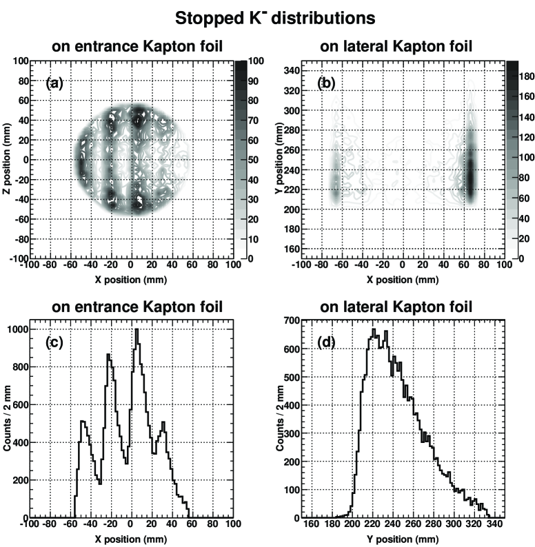
Figure 8: The simulated distributions of the $K^{-}$’s stopped in the (a) entrance and (b) lateral windows made of Kapton. The $x$ axis is set to the direction of the $\phi$ boost. The $z$ axis is parallel to the direction of the beams, and the $y$ axis gives the vertical direction in the setup. (c) and (d) show the projected histograms onto (a) the $x$ axis and (b) the $y$ axis, respectively.

The simulations start with the production of the charged kaon pairs ($K^{+}K^{-}$) at the interaction point (See Fig. 1). Although $\phi$ mesons have decay modes other than $\phi\to K^{+}K^{-}$, they were not needed for the determination of the X-ray yields because the $K^{+}K^{-}$ pairs were efficiently detected experimentally.

The 510 MeV beams of electrons and positrons collide with a crossing angle of 50 mrad (25 mrad per beam) at the interaction point. Thus, the $\phi$ mesons produced have a small transverse momentum of 25.48 MeV/$c$ along the horizontal plane of the colliding beams ($\phi$-boost). The momentum distribution of the $K^{+}K^{-}$ pairs caused by the $\phi$-boost was taken into account in the simulations. The direction of the boost, which is toward the center of the DA$\rm{\Phi}$NE rings, is given by the horizontal direction $x$ in our notation.

The production points of the $\phi$ mesons in DA$\Phi$NE have a finite volume, because of the size and crossing region of the electron and positron beams. The initial distribution of the positions of the $K^{+}K^{-}$ pairs was set to this volume using three-dimensional Gaussians. The broadenings of the Gaussians are as follows: $\sigma_{x}=0.26$ mm, $\sigma_{y}=3.2$ $\mu$m, and $\sigma_{z}=10.4$ mm, where $x,y$ and $z$ give the horizontal, vertical, and beam-axis directions, respectively. The polar angular distribution of the $K^{+}K^{-}$ pairs, which is given as $\rm{d}\sigma/\rm{d}\cos{\theta}\sim\sin^{2}{\theta}$, was taken into account in the simulation.

The interaction processes implemented for kaons were as follows: the decay, elastic scattering, inelastic scattering, and at-rest $K^{-}$ absorption. The photon interactions implemented were the photoelectric effect, Compton and Rayleigh scattering, gamma conversion, bremsstrahlung, and annihilation. In addition, Auger electrons and fluorescence X-rays were produced in the de-excitations of atoms.

13 million $K^{+}K^{-}$ pairs were generated at the interaction point in the simulations, and 1.25 million were recorded in the kaon detector as coincidences. The number of kaon triggers, defined as the number of $K^{+}K^{-}$ events recorded in the kaon detector, is then:

$$N_{trig}^{MC}=1.250\cdot 10^{6}.$$ (5)

The 1.42 g/cm³ density Kapton foils (C₂₂H₁₀N₂O₅) were used as a part of the cylindrical target cell. The foils were placed at two positions: bottom (kaon entrance) and lateral. The number of $K^{-}$’s stopped in the entrance and lateral windows was 24538 and 20858, respectively. The distributions of the $K^{-}$’s stopped in the Kapton windows are plotted in Fig. 8, where the origin of the axes was set to the position of the interaction point.

Figure 8(a) shows the distribution of the $K^{-}$’s stopped in the entrance window. The $z$ axis is parallel to the direction of the beams. The direction of the $\phi$ boost is toward the positive sign of the $x$ axis. The gray scale is proportional to the number of stopped kaons, as indicated in the right side of the figure. The projection of the distribution onto the $x$ axis is shown in Fig. 8(c). The peak structures seen in Fig. 8(c) are due to the use of a degrader having a step-like shape with 2-cm intervals, which was designed to optimize the number of $K^{-}$’s stopping in the gaseous target. The disk-like distribution in Fig. 8(a) comes from the shape of the entrance window, where the distribution of stopped $K^{-}$’s is not uniform. This non-uniformity is due to a combination of the angular dependence of the initial kaon momenta, of the boost effect, and of the shape of the degrader.

The distribution of the $K^{-}$’s stopped in the lateral window is shown in Fig. 8(b), where the $y$ axis gives the vertical direction in the setup. The projection of the distribution onto the $y$ axis is shown in Fig. 8(d). The number of $K^{-}$’s stopped in the boost direction is higher, and the number of $K^{-}$’s stopped in a lower position is also higher.

Table 2: The predicted number of X-rays detected by 94 SDDs in the simulations, where ${ent.}$ and ${lat.}$ denote the origin of the generated X-rays: the entrance (${ent.}$) and lateral (${lat.}$) windows. The number of triggers is $N^{MC}_{trig}=1.25\cdot 10^{6}$. $f_{a}$ is the atomic percentage of each element in Kapton.

Transition	Energy [keV]	$N^{MC}_{ent.}$	$N^{MC}_{lat.}$	$f_{a}\ \$
$K^{-}$C $5\to 4$	10.2165	501	738	22/39
$K^{-}$C $6\to 5$	5.5449	385	600	22/39
$K^{-}$C $6\to 4$	15.7594	428	601	22/39
$K^{-}$C $7\to 5$	8.8858	499	764	22/39
$K^{-}$C $8\to 6$	5.5096	381	596	22/39
$K^{-}$N $5\to 4$	13.9959	33	65	2/39
$K^{-}$N $6\to 5$	7.5954	47	67	2/39
$K^{-}$O $6\to 5$	9.9687	122	167	5/39
$K^{-}$O $7\to 6$	6.0068	96	147	5/39
$K^{-}$O $7\to 5$	15.9733	97	130	5/39
$K^{-}$O $8\to 6$	9.9027	117	160	5/39

Table 3: Calculated detection efficiencies ($\epsilon^{MC}$) of the kaonic atom X-rays produced in Kapton. The systematic errors were calculated using the uncertainties of the position of the experimental apparatus ($\pm 1$cm) and the thicknesses of the degrader ($\pm 50\mu$m). The total errors of the efficiencies, which were obtained by the combination of the statistical and systematic errors, are given in the last column.

Transition	Energy	Efficiency	Stat. error	Syst. error		Total error
	[keV]	[%]	[%]	[%]		[%]
$K^{-}$C $5\to 4$	10.2165	0.1760	$\pm 0.0040$	+0.0407	-0.0106	+0.0409	-0.0113
$K^{-}$C $6\to 5$	5.5449	0.1398	$\pm 0.0036$	+0.0248	-0.0126	+0.0251	-0.0131
$K^{-}$C $6\to 4$	15.7594	0.1462	$\pm 0.0037$	+0.0135	-0.0201	+0.0140	-0.0205
$K^{-}$C $7\to 5$	8.8858	0.1792	$\pm 0.0041$	+0.0318	-0.0192	+0.0321	-0.0196
$K^{-}$C $8\to 6$	5.5096	0.1387	$\pm 0.0036$	+0.0253	-0.0119	+0.0256	-0.0125
$K^{-}$N $5\to 4$	13.9959	0.1558	$\pm 0.0126$	+0.0316	-0.0046	+0.0341	-0.0134
$K^{-}$N $6\to 5$	7.5954	0.1782	$\pm 0.0135$	+0.0190	-0.0278	+0.0233	-0.0309
$K^{-}$O $6\to 5$	9.9687	0.1812	$\pm 0.0086$	+0.0326	-0.0165	+0.0337	-0.0186
$K^{-}$O $7\to 6$	6.0068	0.1523	$\pm 0.0079$	+0.0207	-0.0191	+0.0222	-0.0207
$K^{-}$O $7\to 5$	15.9733	0.1421	$\pm 0.0076$	+0.0149	-0.0195	+0.0168	-0.0210
$K^{-}$O $8\to 6$	9.9027	0.1735	$\pm 0.0084$	+0.0448	-0.0089	+0.0456	-0.0123

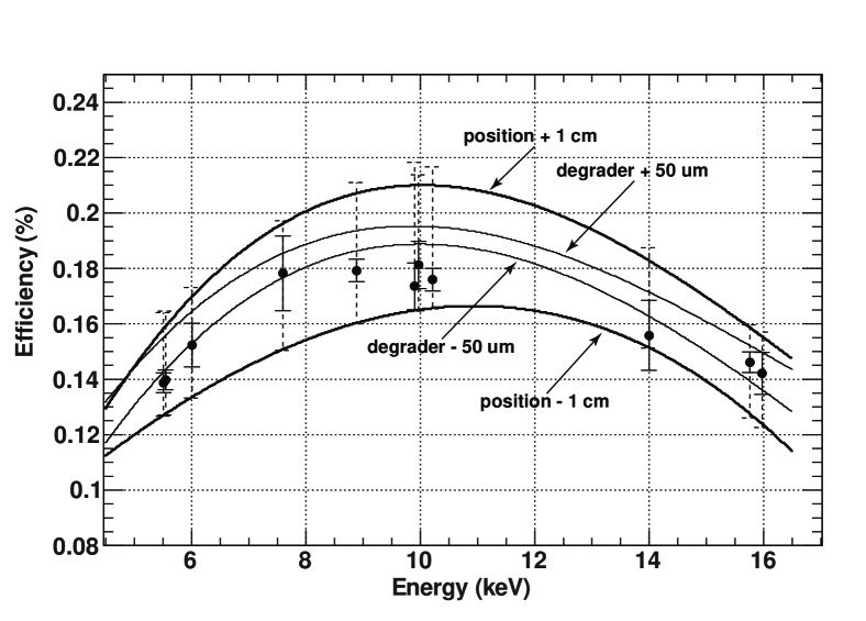
Figure 9: Detection efficiencies ($\epsilon^{MC}$) determined by the simulations. A black circle gives the central value of the efficiency. A solid-line error bar gives the statistical error in the simulation. The efficiencies, when the distance between the interaction point of DA$\Phi$NE and the experimental apparatus were changed by $\pm 1$cm, are shown as the curves indicated by arrows. The efficiencies caused by the uncertainty of the degrader thicknesses ($\pm 50\mu$m) are also shown. A broken-line bar shows the systematic error caused by the combination of the uncertainties of the distance in the setup and degrader thicknesses.

The process of modeling X-ray generation from kaonic atoms was done in the at-rest process of the GEANT4 codes. The kaonic atom X-rays were generated at the position where the $K^{-}$ stopped. A $K^{-}$ stopping in Kapton can form a kaonic atom with any of the following atoms: hydrogen (H), carbon (C), nitrogen (N), or oxygen (O). However, the kaon capture ratios of H:C:N:O in the kaonic atoms produced in Kapton are not well known. In the simulations, realistic capture ratios of kaonic atoms were not included. Instead, the ratios were set to be proportional to the atomic ratios in Kapton: e.g., $f_{a}=22/(22+10+2+5)$ for kaonic carbon. The X-rays were isotropically emitted with a 100% yield for each transition and each kaonic atom, where no cascade calculations were involved. The X-ray energies were fixed to values measured experimentally.

Table 2 shows the predicted number of X-rays recorded in the 94 SDDs:

$$N^{MC}_{SDD}=94,$$ (6)

when the X-ray absorption efficiencies of the SDDs were included. These numbers are shown separately for the two production positions in the Kapton windows: (${ent.}$) for the entrance window and (${lat.}$) for the lateral window. The atomic percentages of the elements in Kapton ($f_{a}$) are also given in the table. The values of $N^{MC}_{ent.}$ and $N^{MC}_{lat.}$ are related to $f_{a}$. Because of the small $f_{a}$ for kaonic nitrogen, the number of kaonic nitrogen X-rays generated is small.

The X-rays produced in the entrance window and the X-rays produced in the lateral window cannot be distinguished experimentally. Thus, the sum of the two values, $N^{MC}_{ent.}$ and $N^{MC}_{lat.}$, were used for the comparison with the experimental data. The efficiency in the simulation is defined similarly to Eq. (4):

$$\epsilon^{MC}=\frac{N^{MC}_{X}}{N^{MC}_{trig}}\cdot\frac{1}{f_{a}}=\frac{N^{MC}_{ent.}+N^{MC}_{lat.}}{N^{MC}_{trig}}\cdot\frac{1}{f_{a}},$$ (7)

where $N^{MC}_{X}$ is the sum of $N^{MC}_{ent.}$ and $N^{MC}_{lat.}$. The term $1/f_{a}$ is the factor to normalize with the Kapton compound. Table. 3 shows the efficiencies ($\epsilon^{MC}$), where the statistical errors are related to the number of $K^{+}K^{-}$ pairs generated in the simulation. Figure 9 shows the detection efficiencies ($\epsilon^{MS}$) as a function of X-ray energy. The positions of the black circles show the central values of the efficiencies. The error bars shown as solid lines correspond to the sizes of the statistical errors. The efficiency decreases at lower energies due to higher X-ray attenuation in the Kapton foil (and the target gas) while it decreases at higher energies due to lower X-ray detection efficiencies of the SDDs.

The uncertainties of the parameters used in the simulation give systematic errors in the determination of the efficiencies ($\epsilon^{MC}$). The dominant contribution was found to be the uncertainty in the vertical distance between the interaction point of DA$\Phi$NE and the experimental apparatus, which is estimated to be about $\pm$1 cm. The contribution to the efficiencies due to this uncertainty is shown in Fig. 9, where the curves were determined by a fit to a cubic function. The uncertainty of the degrader thicknesses (about $\pm$50 $\mu$m in Mylar) also contributes to the systematic error, as shown in Fig. 9. Possible other contributions (such as the uncertainties of the beam energy, and the region and angle of the $e^{+}e^{-}$ colliding at the interaction point) are relatively small (about $\pm$0.04%), and are neglected. The errors due to each contribution were calculated using the differences from the central values, and thus the errors are asymmetric. The errors due to the two contributions were added quadratically. The combined errors are given as systematic errors in Table 3. These systematic errors are plotted with broken line error bars in Fig. 9. The total errors consisting of the statistical and systematic errors are shown in the last column of Table. 3.

5 Results and Discussion

The X-ray yield is defined as the X-ray intensity per stopped kaon. However, the positions of the stopping kaons were not measured in the SIDDHARTA experiment. Instead, the number of stopped kaons in Kapton was evaluated in the Monte Carlo simulations. In addition, the X-ray attenuation in the setup materials and the X-ray absorption efficiencies of the SDDs were also calculated in the simulations.

Comparing the efficiencies determined by the measurements ($\epsilon^{EXP}$) and simulations ($\epsilon^{MC}$), the X-ray yields of the kaonic atoms produced in the Kapton compound can be determined. In the comparison, the normalization was performed using the number of $K^{+}K^{-}$ events detected in the kaon detector ($N_{trig}$). The absolute X-ray yield ($Y$) per stopped $K^{-}$ was calculated as:

$$Y=\frac{\epsilon^{EXP}}{\epsilon^{MC}}=\frac{N^{EXP}_{X}/N^{EXP}_{trig}}{N^{MC}_{X}/N^{MC}_{trig}}.$$ (8)

The correction factor, due to the missing events caused by the data analysis and the data acquisition system, was found to be negligible.

Great care was taken in defining X-ray yields in Kapton. When a kaon stops in Kapton (C₂₂H₁₀N₂O₅), it results in X-rays from one of kaonic carbon, nitrogen, oxygen or hydrogen. However, there is a lack of knowledge on which atom first captures the kaon. To account for this, we define the X-ray yields as the number of X-rays per stopped $K^{-}$ in C₂₂H₁₀N₂O₅.

Table 4: X-ray yields $Y$ of the kaonic atoms produced in Kapton. The X-ray yields $Y$ were defined as the number of X-rays per stopped $K^{-}$ in C₂₂H₁₀N₂O₅. The last column gives the X-ray yields $Y$ normalized by the atomic percentages $f_{a}$.

Transition	Energy	Yield ($Y$)	$Y/f_{a}$
	[keV]	[%]	[%]
$K^{-}$C $5\to 4$	10.2165	$9.7^{+0.7}_{-2.3}$	$17.3^{+1.2}_{-4.1}$
$K^{-}$C $6\to 5$	5.5449	$2.2^{+0.6}_{-0.7}$	$4.0^{+1.1}_{-1.2}$
$K^{-}$C $6\to 4$	15.7594	$1.3\pm 0.3$	$2.4\pm 0.5$
$K^{-}$C $7\to 5$	8.8858	$0.2\pm 0.2$	$0.4\pm 0.3$
$K^{-}$C $8\to 6$	5.5096	$0.3\pm 0.6$	$0.5\pm 1.0$
$K^{-}$N $5\to 4$	13.9959	$0.7\pm 0.2$	$14.0^{+3.9}_{-4.8}$
$K^{-}$N $6\to 5$	7.5954	$0.2\pm 0.2$	$4.7^{+3.2}_{-3.1}$
$K^{-}$O $6\to 5$	9.9687	$1.8^{+0.4}_{-0.5}$	$14.2^{+3.0}_{-3.7}$
$K^{-}$O $7\to 6$	6.0068	$0.5\pm 0.2$	$4.2\pm 1.6$
$K^{-}$O $7\to 5$	15.9733	$0.8\pm 0.3$	$6.0\pm 2.6$
$K^{-}$O $8\to 6$	9.9027	$0.3\pm 0.3$	$2.1^{+2.5}_{-2.6}$

Using the values given in Tables 1, 3 and Eq. (1), the absolute X-ray yields of the kaonic atoms produced in the Kapton compound were calculated. The yield of the kaonic carbon ($K^{-}$C) $5\to 4$ transition normalized by C₂₂H₁₀N₂O₅ was determined to be

$$Y(K^{-}{\rm C}\mbox{ }5\to 4)=9.7^{+0.7}_{-2.3}\%,$$ (9)

where the errors were calculated using the statistical errors measured in the experiment and the total errors in the simulations. The systematic errors related to the measurements are negligible.

Table 4 shows the X-ray yields of kaonic carbon ($K^{-}$C), kaonic nitrogen ($K^{-}$N) and kaonic oxygen ($K^{-}$O) produced in Kapton. Comparing the data of the same atoms, the yield increases as $n$ of the transition decreases. This tendency is related to the populations of the kaons during the cascades in the kaonic atoms. The relative ratios of the successive transitions in the same atoms were determined to be

$$\frac{Y(K^{-}{\rm C}\mbox{ }5\to 4)}{Y(K^{-}{\rm C}\mbox{ }6\to 5)} = 4.4\pm 1.2$$ (10)

$$\frac{Y(K^{-}{\rm N}\mbox{ }5\to 4)}{Y(K^{-}{\rm N}\mbox{ }6\to 5)} = 3.0\pm 2.1$$ (11)

$$\frac{Y(K^{-}{\rm O}\mbox{ }6\to 5)}{Y(K^{-}{\rm O}\mbox{ }7\to 6)} = 3.4\pm 1.4$$ (12)

In the calculation of the relative yields, the systematic errors in the simulations were mainly canceled in our case. The dominant contributions to the errors were found to be the statistical errors, and thus the systematic errors are negligible, resulting in the errors given in Eqs. (10)-(12) being smaller than the errors calculated using the values given in Table 4. These values are larger compared to the data given in Ref. [12]. However, it is not easy to discuss a quantitative comparison, because these ratios have a strong $Z$ dependence, as seen in Fig. 9 of  [12].

The X-ray yields $Y$ of kaonic nitrogen are smaller because of the small atomic percentage of nitrogen in Kapton ($f_{a}=2/39$), as expected. The ratios of C:N:O in the X-ray yields are expected to be related to the atomic ratios of Kapton. The X-ray yields normalized by the atomic percentages $f_{a}$ are shown in Table 4. The normalized yields $Y/f_{a}$ of kaonic carbon and kaonic nitrogen are almost the same within the errors both in the $5\to 4$ and $6\to 5$ transitions, while $Y/f_{a}$ of the kaonic oxygen transitions are higher than those of kaonic carbon or kaonic nitrogen both in the $6\to 5$ and $7\to 5$ transitions. The relative ratios of the X-ray transition yields were determined to be

$$\frac{Y(K^{-}{\rm C}\mbox{ }5\to 4)/f_{a}(\rm{C})}{Y(K^{-}{\rm N}\mbox{ }5\to 4)/f_{a}(\rm{N})} = 1.23\pm 0.35$$ (13)

$$\frac{Y(K^{-}{\rm C}\mbox{ }6\to 5)/f_{a}(\rm{C})}{Y(K^{-}{\rm N}\mbox{ }6\to 5)/f_{a}(\rm{N})} = 0.84\pm 0.60$$ (14)

$$\frac{Y(K^{-}{\rm C}\mbox{ }6\to 5)/f_{a}(\rm{C})}{Y(K^{-}{\rm O}\mbox{ }6\to 5)/f_{a}(\rm{O})} = 0.28\pm 0.09$$ (15)

The systematic errors in the simulations were found to be negligible in the calculation of the relative yields.

The yield patterns and the yield ratios can be related to the capture processes in the Kapton compound and the cascade processes of the kaonic atoms. The capture processes have been studied with several models such as the Fermi-Teller law [24], its improved models [25, 26, 27, 28, 29] and the so-called meso-molecular models [25, 30]. See also Ref. [31]. The hydrogen transfer process could also contribute [15, 16, 32]. Since the X-ray yields are related to the cascade processes in addition to the capture processes, a detailed theoretical calculation is needed to understand the yield patterns determined in this experiment.

6 Conclusions

The kaonic atom X-rays produced in the compound of Kapton ($\rm{C}_{22}\rm{H}_{10}\rm{N}_{2}\rm{O}_{5}$) were measured by the SIDDHARTA collaboration. This is the first measurement of these X-rays using a target made of such a complex compound. Compared to the number of X-rays generated by the Monte Carlo simulations, the absolute X-ray yields of the kaonic atoms produced in Kapton with low atomic numbers $Z$ and high $n$ transitions were determined. We also determined the relative ratios of the successive transitions in the same atoms and the relative ratios of C:N and C:O for the same transitions. These results provide very important information for the theoretical studies of the capture and cascade processes of kaonic atoms in a compound material.

The deduced X-ray yields are also important for the measurement of kaonic deuterium X-rays in the SIDDHARTA-2 experiment [17]. As shown in Fig. 4 of Ref. [17], the kaonic atom X-rays produced in Kapton will be present in the new experiment, although the intensities of the X-rays will be reduced by a factor 20 resulting from the use of a higher density target. One of the difficulties in the extraction of the shift and width of kaonic hydrogen X-rays was the unknown yields of the X-rays produced in Kapton. In the SIDDHARTA-2 experiment, the kaonic deuterium X-rays will be extracted using the X-ray yields determined in this article.

Appendix A Comparison with the experimental data

From the X-ray yields produced in Kapton, it is not simple to extract the X-ray yields of kaonic carbon, nitrogen, and oxygen separately. If we assume that the kaon capture ratios of C:H:N:O are simply proportional to the atomic percentages $f_{a}$ (although this assumption could be incorrect), the normalized yields $Y/f_{a}$ can be compared to the data taken with the targets made of single elements.

The normalized yields $Y/f_{a}$ of kaonic carbon were compared to the data of kaonic carbon taken with the solid target, where the data were given in Ref.[12]. Table 5 shows the comparison. Except for the $6\to 4$ transition, the same transitions were not measured. Despite the simple assumption for the capture ratios, the yields of the $6\to 4$ transition are consistent.

There are two nitrogen data sets with liquid [33] and gas [34] targets. Table 6 shows the comparisons between our results and the nitrogen data. In the yield of the $5\to 4$ transition, our result is consistent with the value given in Ref. [33], while our results are much smaller than the values given by Ref. [34]. Probably, density dependence of the X-ray yields could be also related to the yield patterns.

The oxygen data are not available. Instead, we compare with the data of H₂O, as shown in Table 7. Because reductions of the X-ray yields in the hydride materials were reported [15, 16], these values should be used for reference only.

Table 5: The X-ray yields $Y$ of kaonic carbon produced in Kapton normalized by the atomic percentage $f_{a}$. The X-ray yields shown in the third column were taken from Ref. [12].

Transition	$Y/f_{a}$	Yield
	[%]	[%] [12]
$K^{-}$C $8\to 6$	$0.5\pm 1.0$
$K^{-}$C $6\to 5$	$4.0^{+1.1}_{-1.2}$
$K^{-}$C $7\to 5$	$0.4\pm 0.3$
$K^{-}$C $5\to 4$	$17.3^{+1.2}_{-4.1}$
$K^{-}$C $6\to 4$	$2.4\pm 0.5$	$2.9\pm 1.1$
$K^{-}$C $4\to 3$		$36\pm 6$
$K^{-}$C $5\to 3$		$7.0\pm 1.4$
$K^{-}$C $6\to 3$		$2.8\pm 0.8$
$K^{-}$C $3\to 2$		$2.8\pm 0.8$

Table 6: The X-ray yields $Y$ of kaonic nitrogen produced in Kapton normalized by $f_{a}$. The X-ray yields shown in the third column were taken from Ref. [33]. In the 4th column, the data in the gas target [34] are shown.

Transition	$Y/f_{a}$	Yield	Yield
	[%]	[%] [33]	[%] [34]
$K^{-}$N $7\to 6$			$41.5\pm 8.7{\rm(stat.)}\pm 4.1{\rm(sys.)}$
$K^{-}$N $6\to 5$	$4.7^{+3.2}_{-3.1}$		$55.0\pm 3.9{\rm(stat.)}\pm 5.5{\rm(sys.)}$
$K^{-}$N $5\to 4$	$14.0^{+3.9}_{-4.8}$	$13\pm 4$	$57.4\pm 15.2{\rm(stat.)}\pm 5.7{\rm(sys.)}$
$K^{-}$N $6\to 4$		$4.0\pm 1.7$
$K^{-}$N $4\to 3$		$38\pm 6$
$K^{-}$N $5\to 3$		$3.4\pm 1.0$
$K^{-}$N $6\to 3$		$2.1\pm 0.7$
$K^{-}$N $3\to 2$		$2.5\pm 0.9$

Table 7: The X-ray yields $Y$ of kaonic oxygen produced in Kapton normalized by $f_{a}$. The X-ray yields shown in the third column were taken from Ref. [12], where the target was H₂O. The yield of the $6\to 5$ transition in Ref. [12] includes the yield of the $8\to 6$ transition.

Transition	$Y/f_{a}$	Yield
	[%]	[%] [12]
$K^{-}$O $7\to 6$	$4.2\pm 1.6$
$K^{-}$O $8\to 6$	$2.1^{+2.5}_{-2.6}$	(see caption)
$K^{-}$O $6\to 5$	$14.2^{+3.0}_{-3.7}$	$27\pm 10$
$K^{-}$O $7\to 5$	$6.0\pm 2.6$	$2.0\pm 1.1$
$K^{-}$O $5\to 4$		$13\pm 2$
$K^{-}$O $6\to 4$		$3.1\pm 0.7$
$K^{-}$O $7\to 4$		$1.4\pm 0.5$
$K^{-}$O $4\to 3$		$15\pm 2$
$K^{-}$O $5\to 3$		$3.4\pm 0.6$
$K^{-}$O $6\to 3$		$2.2\pm 0.4$
$K^{-}$O $7\to 3$		$1.4\pm 0.3$
$K^{-}$O $8\to 3$		$0.6\pm 0.2$

References

- [1] SIDDHARTA Collaboration, Phys. Lett. B 704 (2011) 113.
- [2] SIDDHARTA Collaboration, Phys. Lett. B 681 (2009) 310.
- [3] SIDDHARTA Collaboration, Phys. Lett. B 697 (2011) 199.
- [4] SIDDHARTA Collaboration, Phys. Lett. B 714 (2012) 40.
- [5] E. Friedman, et al., Nucl. Phys. A 579 (1994) 518
- [6] E. Friedman, Hyp. Inter. 209 (2012) 127.
- [7] E. Friedman and A. Gal, Nucl. Phys. A 881 (2012) 150.
- [8] E. Friedman and A. Gal, Nucl. Phys. A 899 (2013) 60.
- [9] C. Wiegand, Phys. Rev. Lett. 22 (1969) 1235.
- [10] C. Wiegand and G. Godfrey, Lowrence Berkeley Laboratory report No. LBL-1074.
- [11] M. Leon and R. Seki, Phys. Rev. Lett. 32 (1974) 132.
- [12] C. E. Wiegand, G. L. Godfrey, Phys. Rev. A 9 (1974) 2282.
- [13] R. Kunselman et al., Phys. Rev. Lett. 36 (1976) 446, and reference therein.
- [14] G.T. Condo, Phys. Rev. Lett. 33 (1974) 126.
- [15] G.L. Godfrey and C.E. Wiegand, Phys. Lett. B 56 (1975) 255.
- [16] C.E. Wiegand et al., Phys. Rev. A 15 (1977) 1780.
- [17] M. Bazzi et al., Nucl. Phys. A 907 (2013) 69.
- [18] C. T. Chantler, et al., Phys. Rev. A 73 (2006) 012508.
- [19] G. Hölzer, et al., Phys. Rev. A 56 (1997) 4554.
- [20] A Servomaa and O Keski-Rahkonen, J. Phys. C 8 (1975) 4124.
- [21] J. L. Campbell, et al., Phys. Rev. A 33 (1986) 2410.
- [22] M. Budnar, et al., Nucl. Instrum. Methods B 63 (1992) 377.
- [23] S. Agostinelli et al., Nucl. Instrum. Methods A 506 (2003) 250.
- [24] E. Fermi and E. Teller, Phys. Rev. 72 (1947) 399.
- [25] H. Schneuwly, et al., Nucl. Phys A 312 (1978) 419.
- [26] Z. V. Krumshtein, et al., JETP(Sov. Phys.) 27 (1968) 906.
- [27] H. Daniel, Phys. Rev. Lett. 35 (1975) 1649.
- [28] P. Vogel, et al., Nucl. Phys. A 254 (1975) 455.
- [29] V. I. Petruhkin, et al., JETP(Sov. Phys.) 28 (1969) 1151; JETP(Sov. Phys.) 43 (1976) 595.
- [30] L. I. Ponomarev, Annu. Rev. Nucl. Sci. 23 (1973) 395.
- [31] S. Stanislaus, Nucl. Phys. A 475 (1987) 642.
- [32] D. F. Jackson et al., Phys. Rev. A 25 (1982) 3262.
- [33] G.L. Godfrey and C.E. Wiegand, Lowrence Berkeley Laboratory report No. LBL-3080 (1974), unpublished.
- [34] T. Ishiwatari et al., Phys. Lett. B 593 (2004) 48.