Backpropagation Imaging in Nonlinear Harmonic Holography in the Presence of Measurement and Medium Noises

Abstract

In this paper, the detection of a small reflector in a randomly heterogenous medium using second-harmonic generation is investigated. The medium is illuminated by a time-harmonic plane wave at frequency $\omega$. It is assumed that the reflector has a non-zero second-order nonlinear susceptibility, and thus emits a wave at frequency $2\omega$ in addition to the fundamental frequency linear scattering. It is shown how the fundamental frequency signal and the second-harmonic signal propagate in the medium. A statistical study of the images obtained by migrating the boundary data is performed. It is proved that the second-harmonic image is more stable with respect to medium noise than the one obtained with the fundamental signal. Moreover, the signal-to-noise ratio for the second-harmonic image does not depend neither on the second-order susceptibility tensor nor on the volume of the particle.

Mathematics Subject Classification (MSC2000): 35R30, 35B30

Keywords: wave imaging, harmonic holography, second-harmonic generation, medium noise, resolution, stability

1 Introduction

Second-harmonic microscopy is a promising imaging technique based on a phenomenon called second-harmonic generation (SHG) or frequency-doubling. SHG requires an intense laser beam passing through a material with non vanishing second-order susceptibility [19]. A second electromagnetic field is emitted at exactly twice the frequency of the incoming field. Roughly speaking,

$$\mathbf{E}_{2\omega}\sim\mathbf{E}_{\omega}\chi^{(2)}\mathbf{E}_{\omega},$$ (1)

where $\chi^{(2)}$ is the second-order susceptibility tensor. A condition for an object to have non vanishing second-order susceptibility tensor is to have a noncentrosymmetric structure. Thus SHG only occurs in a few types of physical bodies: crystals [26], interfaces like cell membranes [20, 15], nanoparticle [32, 23], and natural structures like collagen or neurons [14, 24]. This makes SHG a very good contrast mechanism for microscopy, and has been used in biomedical imaging. SHG signals have a very low intensity because the coefficients in $\chi^{(2)}$ have a typical size of picometer $/V$ [16]. This is the reason why a high intensity laser beam is required in order to produce a second-harmonic field that is large enough to be detected by the microscope. Second-harmonic microscopy has several advantages. Among others, the fact that the technique does not involve excitation of molecules so it is not subject to phototoxicity effect or photobleaching. The excitation uses near infrared light which has a very good penetration capacity, and a lot of natural structures (like collagen for instance) exhibit strong SHG properties, so there is no need for probes or dyes in certain cases. SHG images can be collected simultaneously with standard microscopy and two-photon-excitation-fluorescence microscopy for membrane imaging (see, for instance, [15]).

The coherent nature of the SHG signal allows us to use nonlinear holography for measuring the complex two-dimensional (amplitude and phase) SHG signal [22, 28]. The idea is quite similar to conventional linear holography [17, 29]. A frequency doubling crystal is used to produce a coherent reference beam at the second-harmonic frequency, which allows to measure the phase of the one emitted from the reflector [21].

On the other hand, since only the dye/membrane produces the second-harmonic signal, SHG microscopy allows a precise imaging of the dye/membrane, clear from any scattering from the surrounding medium, contrary to the fundamental frequency image, where the signal measured is produced by both the reflector and the medium. As it will be shown in this paper, this is the main feature which makes second-harmonic imaging very efficient when it is not possible to obtain an image of the medium without the dye in order to filter the medium noise. In practical situations [21], it is not possible to get an image without the reflector. The main purpose of this work is to justify that the second-harmonic generation acts in such situations as a powerful contrast imaging approach.

More precisely, we study the case of a nanoparticle with non vanishing second-order susceptibility tensor $\chi^{(2)}$ embedded in a randomly heterogeneous medium illuminated by an incoming electromagnetic field at a fixed frequency $\omega$. We give asymptotic formulas for the electromagnetic field diffracted by the particle and the medium at the fundamental frequency and at the second-harmonic frequency. Then we use a backpropagation algorithm in order to recover the position of the particle from boundary measurements of the fields. We study the images obtained by backpropagation both in terms of resolution and stability. In particular, we elucidate that the second-harmonic field provides a more stable image than that from fundamental frequency imaging, with respect to medium noise, and that the signal-to-noise ratio for the second-harmonic image does not depend neither on $\chi^{(2)}$ nor on the volume of the particle. The aforementioned are the main findings of this study.

The paper is organized as follows. In section 2 we formulate the problem of SHG. In section 3, asymptotic expansions in terms of the size of the small reflector (the nanoparticle) of the scattered field at the fundamental frequency and the second-harmonic generated field are derived. In section 4, we introduce backpropagation imaging functions for localizing the point reflector using the scattered field at the fundamental frequency as well as the second-harmonic field. In section 5, we perform a stability and resolution analysis of the backpropagation imaging functions. We show that the medium noise affects the stability and resolution of the imaging functions in different ways. We prove that using the second-harmonic field renders enhanced stability for the reconstructed image. Our main findings are delineated by a few numerical examples in section 6. The paper ends with a short discussion.

2 Problem formulation

Consider a small electric reflector $\Omega_{r}$ embedded in a randomly heterogeneous medium in $\mathbb{R}^{2}$. We assume that the medium has random fluctuations described by a random process $\mu$ with Gaussian statistics and mean zero. Furthermore, we assume that $\mu$ is compactly supported in $\mathbb{R}^{2}$ and let $\Omega_{\mu}:=\mbox{supp}(\mu)$. We also assume that the refractive index of the background homogeneous medium $\mathbb{R}^{2}\setminus\overline{\Omega_{\mu}}$ is $1$. The medium is illuminated by a plane wave at frequency $\omega>0$, intensity $U_{I}>0$, and direction $\theta\in\mathbb{S}^{1}$:

$$U_{0}(x)=U_{I}e^{i\omega\theta\cdot x},$$ (2)

with $\mathbb{S}^{1}$ being the unit circle. We assume that the incoming plane wave is polarized in the transverse magnetic direction. The small reflector $\Omega_{r}$ is in $\Omega_{\mu}$ and has a refractive index given by

$$[\sigma_{r}-1]\textbf{1}_{\Omega_{r}}(x),$$ (3)

where $\sigma_{r}$ is the refractive index contrast of the reflector, $\Omega_{r}$ is compactly supported in $\Omega_{\mu}$ with volume $|\Omega_{r}|$, and $\textbf{1}_{\Omega_{r}}$ is the characteristic function of $\Omega_{r}$. The squared refractive index $n(x)$ in the whole space has then the following form:

$$\frac{1}{n(x)}=\left(1+\mu(x)+[\sigma_{r}-1]\textbf{1}_{\Omega_{r}}(x)\right).$$ (4)

The scattered field $u_{s}$ generated by the plane wave satisfies the Helmholtz equation:

$$\left\{\begin{aligned} \nabla\cdot\left(([{\sigma_{r}}-1]\textbf{1}_{\Omega_{r}}+\mu+1)\nabla(u_{s}+U_{0})\right)+\omega^{2}(u_{s}+U_{0})=0\quad\mbox{in }\mathbb{R}^{2},\\ \lim\limits_{|x|\to\infty}\sqrt{|x|}(\frac{\partial u_{s}}{\partial|x|}-i\omega u_{s})=0,\end{aligned}\right.$$ (5)

The point reflector also scatters a second field $v$ at frequency $2\omega$. The field $v$ satisfies, up to $O(||\mu||^{2}_{L^{\infty}(\Omega_{\mu})})$, the following Helmholtz equation [13, 19, 31]:

$$\left\{\begin{aligned} \left(\Delta+\frac{(2\omega)^{2}}{[\sigma_{r}-1]\textbf{1}_{\Omega_{r}}+1}(1-\frac{\mu}{[\sigma_{r}-1]\textbf{1}_{\Omega_{r}}+1})\right)v=\sum_{k,l=1,2}\chi_{kl}\partial_{x_{k}}U\partial_{x_{l}}U\textbf{1}_{\Omega_{r}}\quad\mbox{in }\mathbb{R}^{2},\\ \lim\limits_{|x|\to\infty}\sqrt{|x|}\left(\frac{\partial v}{\partial|x|}-2i\omega v\right)=0,\end{aligned}\right.$$ (6)

where $\chi$ is the electric polarization of the reflector, and can be written as $\chi(x)=(\chi_{ij})_{i,j=1,2}\mathbf{1}_{\mbox{r}}(x)$ and $U=u_{s}+U_{0}$ is the total field. Here the second-harmonic field is assumed to be in the transverse electric mode. The polarization of the second-harmonic field is given by symmetry properties of the second-order susceptibility tensor $\chi$. This transverse magnetic–transverse electric polarization mode is known to be supported by a large class of optical nonlinear materials [30]. We choose this polarization mode so that a two-dimensional study of the second harmonic generation with scalar fields would be possible. The results would be pretty similar in a general three-dimensional case, but the computations would be much elusive. The coupled problems (5) and (6) have been mathematically investigated in [9, 10, 11].

Let us consider $\Omega$ to be a domain large enough so that $\Omega_{\mu}=\mbox{supp}(\mu)\Subset\Omega$ and measure the fields $u_{s}$ and $v$ on its boundary $\partial\Omega$. The goal of the imaging problem is to locate the reflector from the far-field measurements of the scattered field $u_{s}$ at the fundamental frequency and/or the second-harmonic generated field $v$. It will be shown in this paper that the use of the second-harmonic field yields a better stability properties than the use of the scattered field at the fundamental frequency in the presence of medium noise.

3 Small-volume expansions

In this section, we establish small-volume expansions for the solutions of problems (5) and (6). We assume that the reflector is of the form $\Omega_{r}=z_{r}+\delta B$, where its characteristic size $\delta$ is small, $z_{r}$ is its location, and $B$ is a smooth domain such that $B\subset B(0,1)$.

3.1 Fundamental frequency problem

Let $U^{(\mu)}=u_{s}^{(\mu)}+U_{0}$ be the total field that would be observed in the absence of any reflector. The scattered field $u_{s}^{(\mu)}$ satisfies

$$\left\{\begin{aligned} \nabla\cdot\left((1+\mu)\nabla(u^{(\mu)}_{s}+U_{0})\right)+\omega^{2}(u^{(\mu)}_{s}+U_{0})=0\quad\mbox{in }\mathbb{R}^{2},\\ \lim\limits_{|x|\to\infty}\sqrt{|x|}(\frac{\partial u^{(\mu)}_{s}}{\partial|x|}-i\omega u^{(\mu)}_{s})=0.\end{aligned}\right.$$ (7)

Therefore,

$$\nabla\cdot(1+\mu)\nabla u^{(\mu)}_{s}+\omega^{2}u^{(\mu)}_{s}=-\nabla\cdot\mu\nabla U_{0}\quad\mbox{in }\mathbb{R}^{2}.$$

Since $\Omega_{\mu}\Subset\Omega$, the following estimate holds

$$||u_{s}^{(\mu)}||_{H^{1}(\Omega)}\leq C||\mu||_{L^{\infty}}$$ (8)

for some positive constant $C$ independent of $\mu$. Here, $H^{1}(\Omega)$ is the set of functions in $L^{2}(\Omega)$, whose weak derivatives are in $L^{2}(\Omega)$. We refer the reader to Appendix A for a proof of (8), which uses the same arguments as those in [1, 2]. Actually, one can prove that

$$u_{s}^{(\mu)}(x)=-\int_{\Omega_{\mu}}\mu(y)\nabla U_{0}(y)\cdot\nabla G^{(0)}_{\omega}(x,y)dy+O(||\mu||_{L^{\infty}}^{2}),\quad x\in\Omega.$$

Moreover, writing

$$\nabla\cdot\left((1+\mu)\nabla(u^{(\mu)}_{s}+U_{0})\right)=-\omega^{2}(u^{(\mu)}_{s}+U_{0}),$$

it follows by using Meyers’ theorem [25] (see also [12, pp. 35-45]) that there exists $\eta>0$ such that for all $0\leq\eta^{\prime}\leq\eta$,

$$\begin{array}[]{lll}||\nabla u_{s}^{(\mu)}||_{L^{2+\eta^{\prime}}(\Omega^{\prime})}&\leq&||\nabla(u_{s}^{(\mu)}+U_{0})||_{L^{2+\eta^{\prime}}(\Omega)}+||\nabla U_{0}||_{L^{2+\eta^{\prime}}(\Omega)}\\ \vskip 6.0pt plus 2.0pt minus 2.0pt\cr&\leq&C||u_{s}^{(\mu)}+U_{0}||_{L^{2+\eta^{\prime}}(\Omega)}+||\nabla U_{0}||_{L^{2+\eta^{\prime}}(\Omega)}\\ \vskip 6.0pt plus 2.0pt minus 2.0pt\cr&\leq&C||u_{s}^{(\mu)}||_{L^{2+\eta^{\prime}}(\Omega)}+C^{\prime}\end{array}$$

for some positive constants $C$ and $C^{\prime}$, where $\Omega^{\prime}\Subset\Omega$. From the continuous embedding of $H^{1}(\Omega)$ into $L^{2+\eta^{\prime}}(\Omega)$ and (8) we obtain

$$||u_{s}^{(\mu)}||_{L^{2+\eta^{\prime}}(\Omega)}\leq C^{\prime\prime},$$

for some constant $C^{\prime\prime}$ independent of $\mu$. Therefore,

$$||\nabla u_{s}^{(\mu)}||_{L^{2+\eta^{\prime}}(\Omega^{\prime})}\leq C$$ (9)

for some constant $C$ independent of $\mu$.

Now, on one hand, by subtracting (5) from (7), we get

$$\nabla\cdot\left(([{\sigma_{r}}-1]\textbf{1}_{\Omega_{r}}+\mu+1)\nabla(u_{s}-u_{s}^{(\mu)})\right)+\omega^{2}(u_{s}-u_{s}^{(\mu)})=-\nabla\cdot[{\sigma_{r}}-1]\textbf{1}_{\Omega_{r}}\nabla U_{0}\\ -\nabla\cdot[{\sigma_{r}}-1]\textbf{1}_{\Omega_{r}}\nabla u_{s}^{(\mu)}\quad\mbox{in }\mathbb{R}^{2}.$$ (10)

On the other hand, we have

$$\begin{array}[]{lll}||[{\sigma_{r}}-1]\textbf{1}_{\Omega_{r}}\nabla u_{s}^{(\mu)}||_{L^{2}(\Omega)}&\leq&\displaystyle C|\Omega_{r}|^{\frac{\eta}{8+2\eta}}||\nabla u_{s}^{(\mu)}||_{L^{2+\frac{\eta}{2}}(\Omega)}\\ \vskip 6.0pt plus 2.0pt minus 2.0pt\cr&\leq&C|\Omega_{r}|^{\frac{\eta}{8+2\eta}}||\nabla u_{s}^{(\mu)}||_{L^{2}(\Omega)}^{\frac{1}{4+\eta}}||\nabla u_{s}^{(\mu)}||_{L^{2+\eta}(\Omega)}^{\frac{1}{4+\eta}},\\ \end{array}$$

and hence, by (8) and (9), we arrive at

$$||[{\sigma_{r}}-1]\textbf{1}_{\Omega_{r}}\nabla u_{s}^{(\mu)}||_{L^{2}(\Omega)}\leq C|\Omega_{r}|^{\frac{\eta}{8+2\eta}}||\mu||_{L^{\infty}}^{\frac{2}{4+\eta}}.$$

Therefore, we can neglect in (10) the term $\nabla\cdot[{\sigma_{r}}-1]\textbf{1}_{\Omega_{r}}\nabla u_{s}^{(\mu)}$ as $||\mu||_{L^{\infty}}\rightarrow 0$.

Let $w^{(\mu)}$ be defined by

$$\begin{array}[]{l}\displaystyle\nabla\cdot(1+\mu+[\sigma_{r}-1]\textbf{1}_{\Omega_{r}})\nabla w^{(\mu)}+\omega^{2}w^{(\mu)}=\nabla\cdot[{\sigma_{r}}-1]\textbf{1}_{\Omega_{r}}\nabla(x-z_{r})\quad\mbox{in }\mathbb{R}^{2},\end{array}$$ (11)

subject to the Sommerfeld radiation condition. Using the Taylor expansion

$$U_{0}(x)=U_{0}(z_{r})+(x-z_{r})\cdot\nabla U_{0}(z_{r})+O(|x-z_{r}|^{2}),$$

one can derive the inner expansion

$$(u_{s}-u_{s}^{(\mu)})(x)=w^{(\mu)}(x)\cdot\nabla U_{0}(z_{r})+O(\delta^{2}),$$ (12)

for $x$ near $z_{r}$. The following estimate holds. We refer the reader to Appendix B for its proof.

Proposition 3.1

There exists a positive constant $C$ independent of $\delta$ such that

$$||u_{s}-u_{s}^{(\mu)}-w^{(\mu)}(x)\cdot\nabla U_{0}(z_{r})||_{H^{1}(\Omega)}\leq C\delta^{2}.$$

Let $G_{\omega}^{(\mu)}$ be the outgoing Green function in the random medium, that is, the solution to

$$(\nabla\cdot(1+\mu)\nabla+\omega^{2})G_{\omega}^{(\mu)}(.,z)=-\delta_{z}\ \quad\mbox{in }\mathbb{R}^{2},$$ (13)

subject to the Sommerfeld radiation condition. Here, $\delta_{z}$ is the Dirac mass at $z$. An important property satisfied by $G_{\omega}^{(\mu)}$ is the reciprocity property [6]:

$$G_{\omega}^{(\mu)}(x,z)=G_{\omega}^{(\mu)}(z,x),\qquad x\neq z.$$ (14)

Let us denote by $G_{\omega}^{(0)}$ the outgoing background Green function, that is, the solution to

$$(\Delta+\omega^{2})G_{\omega}^{(0)}(.,z)=-\delta_{z}\ \qquad\mbox{in }\mathbb{R}^{2},$$ (15)

subject to the Sommerfeld radiation condition.

The Lippmann-Schwinger representation formula:

$$\begin{array}[]{lll}(G_{\omega}^{(\mu)}-G_{\omega}^{(0)})(x,z_{r})&=&\displaystyle\int_{\Omega_{\mu}}\mu(y)\nabla G_{\omega}^{(\mu)}(y,z_{r})\cdot\nabla G_{\omega}^{(0)}(x,y)\,dy\\ \vskip 6.0pt plus 2.0pt minus 2.0pt\cr&=&\displaystyle\int_{\Omega_{\mu}}\mu(y)\nabla G_{\omega}^{(0)}(y,z_{r})\cdot\nabla G_{\omega}^{(0)}(x,y)\,dy\\ \vskip 6.0pt plus 2.0pt minus 2.0pt\cr&&\displaystyle+\int_{\Omega_{\mu}}\mu(y)\nabla(G_{\omega}^{(\mu)}-G_{\omega}^{(0)})(y,z_{r})\cdot\nabla G_{\omega}^{(0)}(x,y)\,dy\end{array}$$

holds for $x\in\partial\Omega$. Since $\Omega_{\mu}\Subset\Omega$, we have

$$\begin{array}[]{l}\displaystyle\bigg{|}(G_{\omega}^{(\mu)}-G_{\omega}^{(0)})(x,z_{r})-\int_{\Omega_{\mu}}\mu(y)\nabla G_{\omega}^{(0)}(y,z_{r})\cdot\nabla G_{\omega}^{(0)}(x,y)\,dy\bigg{|}\leq\\ \vskip 6.0pt plus 2.0pt minus 2.0pt\cr\qquad\displaystyle||\mu||_{L^{\infty}}||\nabla G_{\omega}^{(0)}(x,\cdot)||_{L^{\infty}(\Omega_{\mu})}||\nabla(G_{\omega}^{(\mu)}-G_{\omega}^{(0)})(\cdot,z_{r})||_{L^{2}(\Omega_{\mu})}.\end{array}$$

Similarly to (8), one can prove that

$$||\nabla(G_{\omega}^{(\mu)}-G_{\omega}^{(0)})(\cdot,z_{r})||_{L^{2}(\Omega_{\mu})}\leq C||\mu||_{L^{\infty}},$$ (16)

and hence, there exists a positive constant $C$ independent of $\mu$ such that

$$\bigg{|}(G_{\omega}^{(\mu)}-G_{\omega}^{(0)})(x,z_{r})-\int_{\Omega_{\mu}}\mu(y)\nabla G_{\omega}^{(0)}(y,z_{r})\cdot\nabla G_{\omega}^{(0)}(x,y)\,dy\bigg{|}\leq C||\mu||_{L^{\infty}}^{2},$$ (17)

uniformly in $x\in\partial\Omega$.

Since

$$||\nabla\nabla G_{\omega}^{(0)}(x,\cdot)||_{L^{\infty}(\Omega_{\mu})}\leq C$$ (18)

uniformly in $x\in\partial\Omega$, the estimate

$$\bigg{|}\nabla(G_{\omega}^{(\mu)}-G_{\omega}^{(0)})(x,z_{r})-\nabla\int_{\Omega_{\mu}}\mu(y)\nabla G_{\omega}^{(0)}(y,z_{r})\cdot\nabla G_{\omega}^{(0)}(x,y)\,dy\bigg{|}\leq C||\mu||_{L^{\infty}}^{2},$$ (19)

holds in exactly the same way as in (17). Therefore, the following Born approximation holds.

Proposition 3.2

We have

$$\begin{array}[]{lll}\displaystyle G_{\omega}^{(\mu)}(x,z_{r})&=&\displaystyle G_{\omega}^{(0)}(x,z_{r})-\int_{\Omega_{\mu}}\mu(y)\nabla G_{\omega}^{(0)}(y,z_{r})\cdot\nabla G_{\omega}^{(0)}(x,y)\,dy+O(||\mu||_{L^{\infty}}^{2}),\\ \vskip 6.0pt plus 2.0pt minus 2.0pt\cr\displaystyle\nabla G_{\omega}^{(\mu)}(x,z_{r})&=&\displaystyle\nabla G_{\omega}^{(0)}(x,z_{r})-\nabla\int_{\Omega_{\mu}}\mu(y)\nabla G_{\omega}^{(0)}(y,z_{r})\cdot\nabla G_{\omega}^{(0)}(x,y)\,dy+O(||\mu||_{L^{\infty}}^{2})\end{array}$$

uniformly in $x\in\partial\Omega$.

We now turn to an approximation formula for $w^{(\mu)}$ as $||\mu||_{L^{\infty}}\rightarrow 0$. By integrating by parts we get

$$w^{(\mu)}(x)=(1-\sigma_{r})\int_{\Omega_{r}}\nabla(w^{(\mu)}(y)-(y-z_{r}))\cdot\nabla G_{\omega}^{(\mu)}(x,y)\,dy,\quad x\in\mathbb{R}^{2}.$$

Using (18) we have, for $x$ away from $\Omega_{r}$,

$$w^{(\mu)}(x)=(1-\sigma_{r})[\int_{\Omega_{r}}\nabla(w^{(\mu)}(y)-(y-z_{r}))\,dy]\cdot[\nabla G_{\omega}^{(\mu)}(x,z_{r})+O(\delta)].$$ (20)

Now let $\textbf{1}_{B}$ denote the characteristic function of $B$. Let $\widetilde{w}$ be the solution to

$$\left\{\begin{array}[]{l}\displaystyle\nabla\cdot(1+[\sigma_{r}-1]\textbf{1}_{B})\nabla\widetilde{w}=0\quad\mbox{in }\mathbb{R}^{2},\\ \vskip 6.0pt plus 2.0pt minus 2.0pt\cr\widetilde{w}(\widetilde{x})-\widetilde{x}\rightarrow 0\quad\mbox{as }|\xi|\rightarrow+\infty.\\ \end{array}\right.$$ (21)

The following result holds. We refer the reader to Appendix C for its proof.

Proposition 3.3

We have

$$\nabla\left(w^{(\mu)}(y)-(y-z_{r})\right)=\delta\nabla\widetilde{w}(\widetilde{y})+O(\delta[||\mu||_{L^{\infty}}+(\delta\omega)^{2}]),$$ (22)

where the scaled variable

$$\widetilde{y}=\frac{y-z_{r}}{\delta}.$$

From (22), it follows that

$$\int_{\Omega_{r}}\nabla(w^{(\mu)}(y)-(y-z_{r}))\,dy=\delta^{2}\int_{B}\nabla\widetilde{w}(\widetilde{x})\,d\widetilde{x}+O(\delta^{3}[||\mu||_{L^{\infty}}+(\delta\omega)^{2}]).$$ (23)

Define the polarization tensor associated to $\sigma_{r}$ and $B$ by (see [8])

$$M(\sigma_{r},B):=(\sigma_{r}-1)\int_{B}\nabla\widetilde{w}(\widetilde{x})\,d\widetilde{x},$$

where $\widetilde{w}$ is the solution to (21). The matrix $M(\sigma_{r},B)$ is symmetric definite (positive if $\sigma_{r}>1$ and negative if $\sigma_{r}<1$). Moreover, if $B$ is a disk, then $M(\sigma_{r},B)$ takes the form [8]:

$$M(\sigma_{r},B)=\frac{2(\sigma_{r}-1)}{\sigma_{r}+1}|B|I_{2},$$

where $I_{2}$ is the identity matrix.

To obtain an asymptotic expansion of $u_{s}(x)-u_{s}^{(\mu)}(x)$ in terms of the characteristic size $\delta$ of the scatterer, we take the far-field expansion of (12). Plugging formula (23) into (20), we obtain the following small-volume asymptotic expansion.

Proposition 3.4

We have

$$u_{s}(x)=u_{s}^{(\mu)}(x)-\delta^{2}M(\sigma_{r},B)\nabla U_{0}(z_{r})\cdot\nabla G_{\omega}^{(\mu)}(x,z_{r})+O(\delta^{3}[1+||\mu||_{L^{\infty}}+(\delta\omega)^{2}]),$$ (24)

uniformly in $x\in\partial\Omega$.

Finally, using (19) we arrive at the following result.

Theorem 3.1

We have as $\delta$ goes to zero

$$\begin{array}[]{lll}(u_{s}-u_{s}^{(\mu)})(x)&=&-\displaystyle\delta^{2}M(\sigma_{r},B)\nabla U_{0}(z_{r})\cdot\bigg{[}\nabla G_{\omega}^{(0)}(x,z_{r})+\nabla\int_{\Omega_{\mu}}\mu(y)\nabla G_{\omega}^{(0)}(y,z_{r})\cdot\nabla G_{\omega}^{(0)}(x,y)\,dy\bigg{]}\\ \vskip 6.0pt plus 2.0pt minus 2.0pt\cr&&+O(\delta^{3}[1+||\mu||_{L^{\infty}}+(\delta\omega)^{2}]+\delta^{2}||\mu||^{2}_{L^{\infty}}),\end{array}$$ (25)

uniformly in $x\in\partial\Omega$.

Theorem 3.1 shows that the asymptotic expansion (25) is uniform with respect to $\omega$ and $\mu$, provided that $\omega\leq C/\delta$ and $||\mu||_{L^{\infty}}\leq C^{\prime}\sqrt{\delta}$ for two positive constants $C$ and $C^{\prime}$.

3.2 Second-harmonic problem

We apply similar arguments to derive a small-volume expansion for the second-harmonic field at frequency $2\omega$.

Introduce $G_{2\omega}^{(\sigma_{r},\mu)}(.,z)$ the outgoing solution of

$$\left(\Delta+\frac{(2\omega)^{2}}{[\sigma_{r}-1]\textbf{1}_{\Omega_{r}}+1}(1-\frac{\mu}{[\sigma_{r}-1]\textbf{1}_{\Omega_{r}}+1})\right)G_{2\omega}^{(\sigma_{r},\mu)}(.,z)=-\delta_{z}\qquad\mbox{in }\mathbb{R}^{2}.$$

Let $G_{2\omega}^{(0)}$ be the outgoing solution to (15) with $\omega$ replaced by $2\omega$.

Similarly to (25), an asymptotic expansion for $G_{2\omega}^{(\sigma_{r},\mu)}$ in terms of $\delta$ can be derived. We have

$$(G_{2\omega}^{(\sigma_{r},\mu)}-G_{2\omega}^{(\mu)})(x,z)=O(\delta^{2})$$

for $x\neq z$ and $x,z$ away from $z_{r}$. Here $G_{2\omega}^{(\mu)}$ is the solution to (13) with $\omega$ replaced by $2\omega$. Moreover, the Born approximation yields

$$\begin{array}[]{lll}(G_{2\omega}^{(\sigma_{r},\mu)}-G_{2\omega}^{(0)})(x,z)&=&\displaystyle-(2\omega)^{2}\int_{\Omega_{\mu}}\mu(y)G_{2\omega}^{(0)}(y,z)G_{2\omega}^{(0)}(x,y)dy+O(\delta^{2}+||\mu||_{L^{\infty}}^{2})\end{array}$$

for $x\neq z$ and $x,z$ away from $z_{r}$. From the integral representation formula:

$$v(x)=-\int_{\Omega_{r}}\sum_{k,l=1,2}\chi_{kl}\partial_{x_{k}}U(y)\partial_{x_{l}}U(y)G_{2\omega}^{(\sigma_{r},\mu)}(x,y)dy,$$

it follows that

$$v(x)=-\delta^{2}|B|\left(\sum_{k,l}\chi_{kl}\partial_{x_{k}}U(z_{r})\partial_{x_{l}}U(z_{r})\right)G^{(\sigma_{r},\mu)}_{2\omega}(x,z_{r})+O(\delta^{3}),$$ (26)

where $|B|$ denotes the volume of $B$, and hence, keeping only the terms of first-order in $\mu$ and of second-order in $\delta$:

$$v(x)=-\delta^{2}|B|\left(\sum_{k,l}\chi_{kl}\partial_{x_{k}}U(z_{r})\partial_{x_{l}}U(z_{r})\right)\\ \left[G_{2\omega}^{(0)}(x,z_{r})-4\omega^{2}\int_{\Omega}\mu(y)G_{2\omega}^{(0)}(x,y)G_{2\omega}^{(0)}(y,z_{r})dy+O(||\mu||^{2}_{L^{\infty}})\right]+O(\delta^{3}).$$ (27)

We denote by $(S)^{\theta}$ the source term (the source term strongly depends on the angle $\theta$ of the incoming plane wave):

$$(S)^{\theta}=\left(\sum_{k,l}\chi_{kl}\partial_{x_{k}}U(z_{r})\partial_{x_{l}}U(z_{r})\right).$$ (28)

Now, since

$$U(x)=U_{I}e^{i\omega\theta\cdot x}+\int_{\Omega}\mu(y)\nabla G_{\omega}^{(0)}(x,y)\cdot\nabla U_{0}(y)dy+O(||\mu||^{2}_{L^{\infty}}+\delta),$$ (29)

which follows by using the Born approximation and the inner expansion (12), we can give an expression for the partial derivatives of $U$. We have

$$\partial_{x_{k}}U(x)=i\omega\theta_{k}U_{I}e^{i\omega\theta\cdot x}-i\omega\theta\cdot\int_{\Omega}\nabla(\mu(y)e^{i\omega\theta\cdot y})\partial_{x_{k}}G_{\omega}^{(0)}(x,y)dy+O(||\mu||^{2}_{L^{\infty}}+\delta).$$ (30)

We can rewrite the source term as

$$\left(\sum_{k,l}\chi_{k,l}\partial_{x_{k}}U(z_{r})\partial_{x_{l}}U(z_{r})\right)=-\omega^{2}U_{I}^{2}\sum_{k,l}\chi_{kl}\bigg{[}\theta_{k}\theta_{l}e^{i\omega\theta\cdot z_{r}}\\ -\theta_{k}\theta\cdot\int_{\Omega}\nabla(\mu(y)e^{i\omega\theta\cdot y})\partial_{x_{l}}G_{\omega}^{(0)}(z_{r},y)dy-\theta_{l}\theta\cdot\int_{\Omega}\nabla(\mu(y)e^{i\omega\theta\cdot y})\partial_{x_{k}}G_{\omega}^{(0)}(z_{r},y)dy\\ +\theta\cdot\int_{\Omega}\nabla(\mu(y)e^{i\omega\theta\cdot y})\partial_{x_{l}}G_{\omega}^{(0)}(z_{r},y)dy\theta\cdot\int_{\Omega}\nabla(\mu(y)e^{i\omega\theta\cdot y})\partial_{x_{k}}G_{\omega}^{(0)}(z_{r},y)dy\bigg{]}\\ +O(||\mu||^{2}_{L^{\infty}}+\delta).$$ (31)

Assume that $\mu\in\mathcal{C}^{0,\alpha}$ for $0<\alpha<{1/2}$. From

$$\begin{array}[]{lll}\displaystyle\int_{\Omega}\nabla(\mu(y)e^{i\omega\theta\cdot y})\partial_{x_{l}}G_{\omega}^{(0)}(z_{r},y)dy&=&\displaystyle\int_{\Omega}\nabla(\mu(y)e^{i\omega\theta\cdot y}-\mu(z_{r})e^{i\omega\theta\cdot z_{r}})\partial_{x_{l}}G_{\omega}^{(0)}(z_{r},y)dy\\ \vskip 6.0pt plus 2.0pt minus 2.0pt\cr&=&\displaystyle-\int_{\Omega}\nabla\partial_{x_{l}}G_{\omega}^{(0)}(z_{r},y)(\mu(y)e^{i\omega\theta\cdot y}-\mu(z_{r})e^{i\omega\theta\cdot z_{r}})dy\end{array}$$ (32)

one can show that, for $0<\alpha^{\prime}\leq\alpha$, we have [18]

$$\bigg{|}\theta\cdot\int_{\Omega}\nabla(\mu(y)e^{i\omega\theta\cdot y})\partial_{x_{l}}G_{\omega}^{(0)}(z_{r},y)dy\theta\cdot\int_{\Omega}\nabla(\mu(y)e^{i\omega\theta\cdot y})\partial_{x_{k}}G_{\omega}^{(0)}(z_{r},y)dy\bigg{|}\leq C||\mu||^{2}_{\mathcal{C}^{0,\alpha^{\prime}}},$$

where $C$ is a positive constant independent of $\mu$.

So, if we split $(S)^{\theta}$ into a deterministic part and a random part:

$$(S)^{\theta}=(S)_{det}^{\theta}+(S)_{rand}^{\theta}+O(||\mu||^{2}_{\mathcal{C}^{0,\alpha}}+\delta),$$

we get

$$(S)_{det}^{\theta}=-\omega^{2}U_{I}^{2}e^{i2\omega\theta\cdot z_{r}}\sum_{k,l}\chi_{k,l}\theta_{k}\theta_{l},$$ (33)

and

$$\begin{array}[]{lll}\displaystyle(S)_{rand}^{\theta}&=&\displaystyle\omega^{2}\sum_{k,l}\chi_{k,l}\bigg{[}\theta_{k}\theta\cdot\int_{\Omega}\nabla(\mu(y)e^{i\omega\theta\cdot y})\partial_{x_{l}}G_{\omega}^{(0)}(z_{r},y)dy\\ \vskip 6.0pt plus 2.0pt minus 2.0pt\cr&&\displaystyle+\theta_{l}\theta\cdot\int_{\Omega}\nabla(\mu(y)e^{i\omega\theta\cdot y})\partial_{x_{k}}G_{\omega}^{(0)}(z_{r},y)dy\bigg{]}.\end{array}$$ (34)

Finally, we obtain the following result.

Theorem 3.2

Assume that $\mu\in\mathcal{C}^{0,\alpha}$ for $0<\alpha<{1/2}$. Let $0<\alpha^{\prime}\leq\alpha$. The following asymptotic expansion holds for $v$ as $\delta$ goes to zero:

$$v(x)=-\delta^{2}|B|\bigg{(}(S)_{det}^{\theta}\left[G_{2\omega}^{(0)}(x,z_{r})-4\omega^{2}\int_{\Omega}\mu(y)G_{2\omega}^{(0)}(x,y)G_{2\omega}^{(0)}(y,z_{r})dy\right]+(S)_{rand}^{\theta}G_{2\omega}^{(0)}(x,z_{r})\bigg{)}\\ +O(\delta^{3}+\delta^{2}||\mu||^{2}_{\mathcal{C}^{0,\alpha^{\prime}}})$$ (35)

uniformly in $x\in\partial\Omega$.

4 Imaging functional

In this section, two imaging functionals are presented for locating small reflectors. For the sake of simplicity, we assume that $B$ and $\Omega$ are disks centered at $0$ with radius $1$ and $R$, respectively.

4.1 The fundamental frequency case

We assume that we are in possession of the following data: $\{u_{s}(x),\ x\in\partial\Omega\}$. We introduce the reverse-time imaging functional

$$\forall z^{S}\in\Omega,\ I(z^{S})=\int_{\partial\Omega\times\mathbb{S}^{1}}\frac{1}{i\omega}e^{-i\omega\theta\cdot z^{S}}\theta^{\top}\overline{\nabla G_{\omega}^{(0)}(x,z^{S})}u_{s}(x)d\sigma(x)d\sigma(\theta),$$ (36)

where $\top$ denotes the transpose. Introduce the matrix:

$$R_{\omega}(z_{1},z_{2})=\int_{\partial\Omega}\overline{\nabla G_{\omega}^{(0)}(x,z_{1})}\nabla G_{\omega}^{(0)}(x,z_{2})^{\top}d\sigma(x),\qquad z_{1},z_{2}\in\Omega^{\prime}\Subset\Omega.$$ (37)

Using (25), we have the following expansion for $I(z^{S}),z^{S}\in\Omega^{\prime}$,

$$I(z^{S})=\int_{\partial\Omega\times\mathbb{S}^{1}}\frac{1}{i\omega}e^{-i\omega\theta\cdot z^{S}}\theta^{\top}\overline{\nabla G_{\omega}^{(0)}(x,z^{S})}u_{s}^{(\mu)}(x)d\sigma(x)d\sigma(\theta)\\ -\frac{2\pi\delta^{2}(\sigma_{r}-1)}{\sigma_{r}+1}U_{I}\int_{\mathbb{S}^{1}}e^{-i\omega\theta\cdot(z^{S}-z_{r})}\theta^{\top}\bigg{[}R_{\omega}(z^{S},z_{r})\\ \vskip 6.0pt plus 2.0pt minus 2.0pt\cr+\int_{\partial\Omega}\overline{\nabla G_{\omega}^{(0)}(x,z^{S})}\left(\nabla\int_{\Omega_{\mu}}\mu(y)\nabla G_{\omega}^{(0)}(y,z_{r})\cdot\nabla G_{\omega}^{(0)}(x,y)dy\right)^{\top}d\sigma(x)\bigg{]}\theta d\sigma(\theta)\\ +O(\delta^{3}+\delta^{2}||\mu||_{L^{\infty}}^{2}).$$ (38)

Note that

$$\begin{array}[]{l}\displaystyle\int_{\partial\Omega}\overline{\nabla G_{\omega}^{(0)}(x,z^{S})}\left(\nabla\int_{\Omega_{\mu}}\mu(y)\nabla G_{\omega}^{(0)}(y,z_{r})\cdot\nabla G_{\omega}^{(0)}(x,y)dy\right)^{\top}d\sigma(x)\\ \qquad\displaystyle=\int_{\Omega_{\mu}}\mu(y)\int_{\partial\Omega}\overline{\nabla G_{\omega}^{(0)}(x,z^{S})}\left(\nabla\nabla G_{\omega}^{(0)}(x,y)\nabla G_{\omega}^{(0)}(y,z_{r})\right)^{\top}d\sigma(x)dy.\end{array}$$

Remark 4.1

Here, the fact that not only we backpropagate the boundary data but also we average it over all the possible illumination angles in $\mathbb{S}^{1}$ has two motivations. As will be shown later in section 5, the first reason is to increase the resolution and make the peak at the reflector’s location isotropic. If we do not sum over equi-distributed illumination angles over the sphere, we get more of ”8-shaped” spot, as shown in Figure 8. The second reason is that an average over multiple measurements increases the stability of the imaging functional with respect to measurement noise.

Remark 4.2

If we could take an image of the medium in the absence of reflector before taking the real image, we would be in possession of the boundary data $\{u_{s}-u_{s}^{(\mu)},\ x\in\partial\Omega\}$, and thus we would be able to detect the reflector in a very noisy background. But in some practical situations [21], it is not possible to get an image without the reflector. As it will be shown in section 5, second-harmonic generation can be seen as a powerful contrast imaging approach [21]. In fact, we will prove that the second harmonic image is much more stable with respect to the medium noise and to the volume of the particle than the fundamental frequency image.

4.2 Second-harmonic backpropagation

If we write a similar imaging functional for the second-harmonic field $v$, assuming that we are in possession of the boundary data $\{v(x),\ x\in\partial\Omega\}$, we get

$$\forall z^{S}\in\Omega,\ J_{\theta}(z^{S})=\int_{\partial\Omega\times\mathbb{S}^{1}}v(x)\overline{G_{2\omega}^{(0)}(x,z^{S})}e^{-2i\omega\theta\cdot z^{S}}d\sigma(x)d\sigma(\theta).$$ (39)

As before, using (35) we can expand $J$ in terms of $\delta$ and $\mu$. Considering first-order terms in $\delta$ and $\mu$ we get

$$J(z^{S})=-\pi\delta^{2}\int_{\mathbb{S}^{1}}e^{-2i\omega\theta\cdot z^{S}}\bigg{[}(S)_{det}^{\theta}\Big{(}\int_{\partial\Omega}\overline{G_{2\omega}^{(0)}(x,z^{S})}G_{2\omega}^{(0)}(x,z_{r})d\sigma(x)\\ -4\omega^{2}\int_{\partial\Omega}\overline{G_{2\omega}^{(0)}(x,z^{S})}\int_{\Omega}\mu(y)G_{2\omega}^{(0)}(y,x)G_{2\omega}^{(0)}(y,z_{r})dyd\sigma(x)\Big{)}\\ +(S)_{rand}^{\theta}\int_{\partial\Omega}\overline{G_{2\omega}^{(0)}(x,z^{S})}G_{2\omega}^{(0)}(x,z_{r})d\sigma(x)\bigg{]}d\sigma(\theta)+O(\delta^{3}+\delta^{2}||\mu||_{\mathcal{C}^{0,\alpha^{\prime}}}^{2}),$$ (40)

where $0<\alpha^{\prime}\leq\alpha$. Now, if we define $Q_{2\omega}$ as

$$Q_{2\omega}(x,z)=\int_{\partial\Omega}G_{2\omega}^{(0)}(y,x)\overline{G_{2\omega}^{(0)}(y,z)}d\sigma(y).$$ (41)

We have

$$J(z^{S})=-\pi\delta^{2}\int_{\mathbb{S}^{1}}e^{-2i\omega\theta\cdot z^{S}}\bigg{[}(S)_{det}^{\theta}\left(Q_{2\omega}(z_{r},z^{S})-4\omega^{2}\int_{\Omega_{\mu}}\mu(y)G_{2\omega}^{(0)}(y,z_{r})Q_{2\omega}(y,z^{S})dy\right)\\ +(S)_{rand}^{\theta}Q_{2\omega}(z_{r},z^{S})\bigg{]}d\sigma(\theta)+O(\delta^{3}+\delta^{2}||\mu||_{\mathcal{C}^{0,\alpha^{\prime}}}^{2}).$$ (42)

5 Statistical analysis

In this section, we perform a resolution and stability analysis of both functionals. Since the image we get is a superposition of a deterministic image and of a random field created by the medium noise, we can compute the expectation and the covariance functions of those fields in order to estimate the signal-to-noise ratio. For the reader’s convenience we give our main results in the following proposition.

Proposition 5.1

Let $l_{\mu}$ and $\sigma_{\mu}$ be respectively the correlation length and the standard deviation of the process $\mu$. Assume that $l_{\mu}$ is smaller than the wavelength $2\pi/\omega$. Let $(SNR)_{I}$ and $(SNR)_{J}$ be defined by

$$(SNR)_{I}=\frac{\mathbb{E}[I(z_{r})]}{(Var[I(z_{r})])^{1/2}},$$ (43)

and

$$(SNR)_{J}=\frac{\mathbb{E}[J(z_{r})]}{(Var[J(z_{r})])^{\frac{1}{2}}}.$$ (44)

We have

$$(SNR)_{I}\approx\frac{\sqrt{2}\pi^{3/2}\omega\delta^{2}U_{I}}{\sigma_{\mu}l_{\mu}\sqrt{\omega\text{ diam }\Omega_{\mu}}}\frac{|\sigma_{r}-1|}{\sigma_{r}+1},$$ (45)

and

$$(SNR)_{J}\geq\frac{l_{\mu}^{\alpha}\left(\int_{\mathbb{S}^{1}}\left(\sum_{k,l}\chi_{k,l}\theta_{k}\theta_{l}\right)d\theta\right)}{\sqrt{C}\sigma_{\mu}\min(\omega^{-\alpha},1)\max_{k,l}\left|\chi_{k,l}\right|\sqrt{\left(\omega\text{diam }\Omega_{\mu}\right)^{3+2\alpha}+1}}.$$ (46)

Here, diam denotes the diameter, $\alpha$ is the upper bound for Holder-regularity of the random process $\mu$ (see section 5.1).

5.1 Assumptions on the random process $\mu$

Let $z(x)$, $x\in\mathbb{R}^{2}$ be a stationary random process with Gaussian statistics, zero mean, and a covariance function given by $R(|x-y|)$ satisfying $R(0)=\sigma_{\mu}^{2}$, $|R(0)-R(s)|\ \leq\sigma_{\mu}^{2}\frac{s^{2\alpha}}{l_{\mu}^{2\alpha}}$ and $R$ is decreasing. Then, $z$ is a $\mathcal{C}^{0,\alpha^{\prime}}$ process for any $\alpha^{\prime}<\alpha$ ([3, Theorem 8.3.2]). Let $F$ be a smooth odd bounded function, with derivative bounded by one. For example $F=\arctan$ is a suitable choice. Take

$$\mu(x)=F[z(x)].$$

Then $\mu$ is a bounded $\mathcal{C}^{0,\alpha^{\prime}}$ stationary process with zero mean. We want to compute the expectation of its norm. Introduce

$$p(h)=\max_{\|x-y\|\leq\sqrt{2}h}\mathbb{E}|z(x)-z(y)|.$$ (47)

One can also write $p(u)=\sqrt{2}\sqrt{R(0)-R(\sqrt{2}u)}$. According to [3], for all $h,t\in\Omega_{\mu}$, almost surely,

$$|z(t+h)-z(t)|\leq 16\sqrt{2}[\log(B)]^{1/2}p(\frac{|h|}{l_{\mu}})+32\sqrt{2}\int_{0}^{\frac{|h|}{l_{\mu}}}\left(-\log u\right)^{1/2}dp(u),$$ (48)

where $B$ is a positive random variable with $\mathbb{E}[B^{n}]\leq(4\sqrt{2})^{n}$ ([3, Formula 3.3.23]). We have that

$$p(|h|)\leq\sqrt{2}^{1+\alpha}\sigma_{\mu}\frac{|h|^{\alpha}}{l_{\mu}^{\alpha}}.$$ (49)

By integration by parts we find that

$$\int_{0}^{\frac{|h|}{l_{\mu}}}\left(-\log u\right)^{1/2}dp(u)=\left[(-\log u)^{1/2}p(u)\right]_{0}^{\frac{|h|}{l_{\mu}}}+\frac{1}{2}\int_{0}^{\frac{|h|}{l_{\mu}}}(-\log u)^{-1/2}u^{-1}p(u)du.$$ (50)

For any $\varepsilon>0$, since $s^{\varepsilon}\sqrt{-\log s}\leq\frac{1}{\sqrt{\varepsilon}}e^{1/2}$ on $[0,1]$, we have, as $|h|$ goes to $0$, that

$$\left[(-\log u)^{1/2}p(u)\right]_{0}^{\frac{|h|}{l_{\mu}}}\leq e^{\frac{1}{2}}\frac{\sqrt{2}^{1+\alpha}\sigma_{\mu}}{\sqrt{\varepsilon}}\frac{|h|^{\alpha-\varepsilon}}{l_{\mu}^{\alpha}}.$$ (51)

Similarly, when $|h|<\frac{1}{2e}$, for every $0<u<|h|$,

$$(-\log u)^{-1/2}s^{-1}p(u)\leq\sqrt{2}^{1+\alpha}\sigma_{\mu}\frac{u^{\alpha-1}}{l_{\mu}^{\alpha}}.$$

So we get, when $|h|$ goes to $0$, for every $\varepsilon>0$,

$$\int_{0}^{\frac{|h|}{l_{\mu}}}\left(-\log u\right)^{1/2}dp(u)\leq\frac{e^{\frac{1}{2}}\sqrt{2}^{1+\alpha}\sigma_{\mu}}{\sqrt{\varepsilon}}\frac{|h|^{\alpha-\varepsilon}}{l_{\mu}^{\alpha}}+\frac{\sqrt{2}^{1+\alpha}\sigma_{\mu}}{\alpha}\frac{|h|^{\alpha}}{l_{\mu}^{\alpha}}.$$ (52)

Therefore, when $|h|$ goes to zero, we have for any $\varepsilon>0$:

$$|z(t+h)-z(t)|\leq 32\sqrt{2}^{\alpha}\log(B)^{1/2}\sigma_{\mu}\frac{|h|^{\alpha}}{l_{\mu}^{\alpha}}+64e^{\frac{1}{2}}\sqrt{2}^{\alpha}\sigma_{\mu}\frac{1}{l_{\mu}^{\alpha}}\left[\frac{1}{\sqrt{\varepsilon}}|h|^{\alpha-\varepsilon}+\frac{1}{2}|h|^{\alpha}\right].$$ (53)

Since $F^{\prime}\leq 1$, composing by $F$ yields, for any $x,y\in\mathbb{R}^{2}$,

$$|\mu(x)-\mu(y)|\leq|z(x)-z(y)|.$$ (54)

We get the following estimate on $\|\mu\|_{\mathcal{C}^{0,\alpha^{\prime}}}$, for any $\alpha^{\prime}\in]0,\alpha[$, almost surely

$$\sup_{\begin{subarray}{c}x,y\in\Omega_{\mu}\\ |x-y|\leq h\end{subarray}}\frac{|\mu(x)-\mu(y)|}{|x-y|^{\alpha^{\prime}}}\leq 32\sqrt{2}^{\alpha}\log(B)^{1/2}\sigma_{\mu}\frac{h^{\alpha-\alpha^{\prime}}}{l_{\mu}^{\alpha}}+64e^{\frac{1}{2}}\sqrt{2}^{\alpha}\sigma_{\mu}\frac{1}{l_{\mu}^{\alpha}}\left[\frac{1}{\sqrt{\alpha-\alpha^{\prime}}}+\frac{1}{2}h^{\alpha-\alpha^{\prime}}\right]$$ (55)

$$\|\mu\|_{\mathcal{C}^{0,\alpha^{\prime}}}\leq 64\sqrt{2}^{\alpha}\frac{e^{\frac{1}{2}}\left[\log(B)^{1/2}+1\right]}{\sqrt{\alpha-\alpha^{\prime}}}\frac{\sigma_{\mu}}{l_{\mu}^{\alpha}},$$ (56)

which gives, since $\mathbb{E}[\log B]\leq\mathbb{E}[B]-1\leq 4\sqrt{2}-1$

$$\mathbb{E}[\|\mu\|_{\mathcal{C}^{0,\alpha^{\prime}}}^{2}]\leq 64^{2}2^{4+\alpha}\frac{e}{\alpha-\alpha^{\prime}}\frac{\sigma_{\mu}^{2}}{l_{\mu}^{2\alpha}}.$$ (57)

5.2 Standard backpropagation

5.2.1 Expectation

We use (38) and the fact that $\mathbb{E}(\mu)(x)=0,\ \forall x\in\Omega$, to find that

$$\mathbb{E}[I(z^{S})]=-2\pi\delta^{2}\frac{\sigma_{r}-1}{\sigma_{r}+1}U_{I}\int_{\mathbb{S}^{1}}e^{-i\omega\theta\cdot(z^{S}-z_{r})}\theta^{\top}R_{\omega}(z^{S},z_{r})\theta d\theta.$$ (58)

We now use the Helmholtz-Kirchoff theorem. Since (see [6]):

$$\lim_{R\rightarrow\infty}\int_{|x|=R}\nabla G_{\omega}^{(0)}(x,y)\overline{\nabla G_{\omega}^{(0)}(z,y)}^{\top}dy=\frac{1}{\omega}\nabla_{z}\nabla_{x}\text{ Im}\left[G_{\omega}^{(0)}(x,z)\right]$$ (59)

and

$$\text{ Im}\left[G_{\omega}^{(0)}(x,z)\right]=\frac{1}{4}J_{0}(\omega|x-z|),$$ (60)

we can compute an approximation of $R_{\omega}$.

$$\frac{1}{\omega}\nabla_{z}\nabla_{x}\text{ Im}\left[G_{\omega}^{(0)}(x,z)\right]=\frac{1}{4}\bigg{[}\omega J_{0}(\omega|x-z|)\left(\frac{(x-z)}{|x-z|}\frac{(x-z)^{\top}}{|x-z|}\right)\\ -\frac{2J_{1}(\omega|x-z|)}{|x-z|}\left(\frac{(x-z)}{|x-z|}\frac{(x-z)^{\top}}{|x-z|}\right)\\ +\frac{J_{1}(\omega|x-z|)}{|x-z|}I_{2}\bigg{]},$$ (61)

where $I_{2}$ is the $2\times 2$ identity matrix. We can see that $R_{\omega}$ decreases as $|z_{r}-z^{S}|^{-\frac{1}{2}}$. The imaging functional has a peak at location $z^{S}=z_{r}$. Evaluating $R_{\omega}$ at $z^{S}=z_{r}$ we get

$$\ R_{\omega}(z_{r},z_{r})=\frac{\omega}{8}I_{2}.$$ (62)

So we get the expectation of $I$ at point $z_{r}$:

$$\mathbb{E}[I(z_{r})]\approx-\frac{\pi^{2}(\sigma_{r}-1)}{2(\sigma_{r}+1)}\omega\delta^{2}U_{I}.$$ (63)

5.2.2 Covariance

Let

$$\text{Cov}\left(I(z^{S}),I(z^{S^{\prime}})\right)=\mathbb{E}\bigg{[}\left(I(z^{S})-\mathbb{E}[I(z^{S})]\right)\overline{\left(I(z^{S^{\prime}})-\mathbb{E}[I(z^{S^{\prime}})]\right)}\bigg{]}.$$ (64)

Define

$$\widetilde{R}_{\omega}(z^{S},z_{r},y)=\int_{\partial\Omega}\overline{\nabla G_{\omega}^{(0)}(x,z^{S})}\left(\nabla\nabla G_{\omega}^{(0)}(x,y)\nabla G_{\omega}^{(0)}(y,z_{r})\right)^{\top}d\sigma(x).$$ (65)

Using (38) and (63), we get

$$I(z^{S})-\mathbb{E}[I(z^{S})]=\int_{\partial\Omega\times\mathbb{S}^{1}}\frac{1}{i\omega}e^{-i\omega\theta\cdot z^{S}}\theta^{\top}\overline{\nabla G_{\omega}^{(0)}(x,z^{S})^{\top}}u_{s}^{(\mu)}(x)dxd\theta\\ -2\pi\delta^{2}\frac{\sigma_{r}-1}{\sigma_{r}+1}U_{I}\int_{\mathbb{S}^{1}}e^{-i\omega\theta\cdot(z^{S}-z_{r})}\bigg{[}\int_{\Omega}\mu(y)\theta^{\top}\widetilde{R}_{\omega}(z^{S},z_{r},y)\theta dy\bigg{]}d\theta.$$ (66)

The computations are a bit tedious. For brevity, we write the quantity above as

$$I(z^{S})-\mathbb{E}[I(z^{S})]=A_{I}(z^{S})+B_{I}(z^{S}),$$ (67)

with

$$A_{I}(z^{S})=\int_{\partial\Omega\times\mathbb{S}^{1}}\frac{1}{i\omega}e^{-i\omega\theta\cdot z^{S}}\theta^{\top}\overline{\nabla G_{\omega}^{(0)}(x,z^{S})}u_{s}^{(\mu)}(x)dxd\theta,$$ (68)

and

$$B_{I}(z^{S})=-2\pi\delta^{2}\frac{\sigma_{r}-1}{\sigma_{r}+1}U_{I}\int_{\mathbb{S}^{1}}e^{-i\omega\theta\cdot(z^{S}-z_{r})}\bigg{[}\int_{\Omega}\mu(y)\theta^{\top}\widetilde{R}_{\omega}(z^{S},z_{r},y)\theta dy\bigg{]}d\theta.$$ (69)

We now compute each term of the product in (64) separately.

Main speckle term:

We need to estimate the typical size of $A_{I}$. From (8), keeping only terms of first-order in $\mu$ yields

$$A_{I}(z^{S})=-\int_{\partial\Omega\times\mathbb{S}^{1}}\frac{1}{i\omega}e^{-i\omega\theta\cdot z^{S}}\theta^{\top}\overline{\nabla G_{\omega}^{(0)}(x,z^{S})}\int_{\Omega}\mu(y)\nabla G_{\omega}^{(0)}(x,y)\cdot\nabla U_{0}(y)dydxd\theta+O(\|\mu\|_{\infty}^{2}),$$ (70)

so we have:

$$A_{I}(z^{S})=-U_{I}\int_{\Omega\times\mathbb{S}^{1}}e^{-i\omega\theta\cdot(z^{S}-y)}\mu(y)\theta^{\top}R_{\omega}(z^{S},y)\theta dyd\theta,$$ (71)

and hence,

$$A_{I}(z^{S})\overline{A_{I}(z^{S^{\prime}})}=U_{I}^{2}\int_{\mathbb{S}^{1}}e^{-i\omega\theta\cdot(z^{S}-z^{S^{\prime}})}\\ \bigg{[}\int\int_{\Omega\times\Omega}e^{i\omega\theta\cdot(y-y^{\prime})}\mu(y)\mu(y^{\prime})\theta^{\top}R_{\omega}(z^{S},y)\overline{R_{\omega}(z^{S^{\prime}},y^{\prime})}\theta dydy^{\prime}\bigg{]}d\theta.$$ (72)

We assume that the medium noise is localized and stationary on its support $\Omega_{\mu}$. We also assume that the correlation length $l_{\mu}$ is smaller than the wavelength. We note $\sigma_{\mu}$ the standard deviation of the process $\mu$. We can then write:

$$\mathbb{E}\bigg{[}A_{I}(z^{S})\overline{A_{I}(z^{S^{\prime}})}\bigg{]}=U_{I}^{2}\sigma_{\mu}^{2}l_{\mu}^{2}\int_{\mathbb{S}^{1}}e^{i\omega\theta\cdot(z^{S}-z^{S^{\prime}})}\int_{\Omega_{\mu}}\theta^{\top}R_{\omega}(z^{S},y)\overline{R_{\omega}(z^{S^{\prime}},y)}\theta dyd\theta.$$ (73)

We introduce

$$P_{\omega}(z^{S},y,z^{S^{\prime}}):=\int_{\mathbb{S}^{1}}e^{i\omega\theta\cdot(z^{S}-z^{S^{\prime}})}\theta^{\top}R_{\omega}(z^{S},y)\overline{R_{\omega}(z^{S^{\prime}},y)}\theta d\theta,$$ (74)

where $R_{\omega}$ is defined by (37). Therefore, we have

$$\mathbb{E}\bigg{[}A_{I}(z^{S})\overline{A_{I}(z^{S^{\prime}})}\bigg{]}=U_{I}^{2}\sigma_{\mu}^{2}l_{\mu}^{2}\int_{\Omega_{\mu}}P_{\omega}(z^{S},y,z^{S^{\prime}})dy.$$ (75)

Hence, $A_{I}$ is a complex field with Gaussian statistics of mean zero and covariance given by (75). It is a speckle field and is not localized.

We compute its typical size at point $z^{S}=z^{S^{\prime}}=z_{r}$, in order to get signal-to-noise estimates. Using (61), we get that for $|x-z|>>1$:

$$\lim_{R\rightarrow\infty}\int_{|x|=R}\nabla G_{\omega}^{(0)}(x,y)\overline{\nabla G_{\omega}^{(0)}(z,y)}^{\top}dy=\frac{\omega}{4}J_{0}(\omega|x-z|)\left(\frac{(x-z)}{|x-z|}\frac{(x-z)^{\top}}{|x-z|}\right).$$

Since we have, for $|x-z|>>1$,

$$J_{0}(\omega|x-z|)\sim\frac{\sqrt{2}\cos(\omega|x-z|-\frac{\pi}{4})}{\sqrt{\pi\omega|x-z|}},$$ (76)

we obtain that

$$R_{\omega}(x,z)\approx\frac{\sqrt{\omega}\cos(\omega|x-z|-\pi/4)}{2\sqrt{2\pi}}|x-z|^{-1/2}\left(\frac{(x-z)}{|x-z|}\frac{(x-z)^{\top}}{|x-z|}\right)\ \text{for }|x-z|>>1.$$ (77)

Now we can write

$$\mathbb{E}\bigg{[}A_{I}(z_{r})\overline{A_{I}(z_{r})}\bigg{]}\approx U_{I}^{2}\sigma_{\mu}^{2}l_{\mu}^{2}\int_{\Omega_{\mu}}\left(\frac{\sqrt{\omega}}{2\sqrt{2\pi}}\right)^{2}\frac{1}{2}|y-z_{r}|^{-1}\int_{\mathbb{S}^{1}}\theta^{\top}\left(\frac{(y-z_{r})}{|y-z_{r}|}\frac{(y-z_{r})^{\top}}{|y-z_{r}|}\right)\theta d\theta dy.$$ (78)

If we compute the term:

$$\int_{\mathbb{S}^{1}}\theta^{\top}\left(\frac{(y-z_{r})}{|y-z_{r}|}\frac{(y-z_{r})^{\top}}{|y-z_{r}|}\right)\theta d\theta=\int_{0}^{2\pi}\bigg{[}\left(\frac{(y-z_{r})_{1}}{|y-z_{r}|}\right)^{2}\cos^{2}\theta+\left(\frac{(y-z_{r})_{2}}{|y-z_{r}|}\right)^{2}\sin^{2}\theta\bigg{]}d\theta,$$ (79)

then, after linearization and integration, we get

$$\int_{\mathbb{S}^{1}}\theta^{\top}\left(\frac{(y-z_{r})}{|y-z_{r}|}\frac{(y-z_{r})^{\top}}{|y-z_{r}|}\right)\theta d\theta=\pi.$$ (80)

So we have:

$$\mathbb{E}\bigg{[}A_{I}(z_{r})\overline{A_{I}(z_{r})}\bigg{]}\approx\pi U_{I}^{2}\sigma_{\mu}^{2}l_{\mu}^{2}\int_{\Omega_{\mu}}\left(\frac{\sqrt{\omega}}{4\sqrt{\pi}}\right)^{2}|y-z_{r}|^{-1}dy,$$ (81)

and therefore,

$$\mathbb{E}\bigg{[}A_{I}(z_{r})\overline{A_{I}(z_{r})}\bigg{]}\approx\pi\frac{\omega}{8}U_{I}^{2}\sigma_{\mu}^{2}l_{\mu}^{2}\text{diam }\Omega_{\mu}.$$ (82)

Secondary speckle term:

We have

$$B_{I}(z^{S})\overline{B_{I}(z^{S^{\prime}})}=\left(2\pi\delta^{2}\frac{\sigma_{r}-1}{\sigma_{r}+1}U_{I}\right)^{2}\int_{\mathbb{S}^{1}}e^{-i\omega\theta\cdot(z^{S}-z^{S^{\prime}})}\\ \bigg{[}\int_{\Omega}\mu(y)\mu(y^{\prime})\theta^{\top}\widetilde{R}_{\omega}(z^{S},z_{r},y)\overline{\widetilde{R}_{\omega}(z^{S^{\prime}},z_{r},y^{\prime})}\theta dydy^{\prime}\bigg{]}d\theta.$$ (83)

So we get the expectation:

$$\mathbb{E}\bigg{[}B_{I}(z^{S})\overline{B_{I}(z^{S^{\prime}})}\bigg{]}=\left(2\pi\delta^{2}\frac{\sigma_{r}-1}{\sigma_{r}+1}U_{I}\right)^{2}\sigma_{\mu}^{2}l_{\mu}^{2}\\ \int_{\mathbb{S}^{1}}e^{-i\omega\theta\cdot(z^{S}-z^{S^{\prime}})}\theta^{\top}\bigg{[}\int_{\Omega_{\mu}}\widetilde{R}_{\omega}(z^{S},z_{r},y)\overline{\widetilde{R}_{\omega}(z^{S^{\prime}},z_{r},y)}dy\bigg{]}\theta d\theta.$$ (84)

This term also creates a speckle field on the image. As before, we compute the typical size of this term at point $z_{r}$. We first get an estimate on $\widetilde{R}_{\omega}$.

$$|\left(\widetilde{R}_{\omega}(z^{S},z_{r},y)\right)_{i,j}|\leq|\partial_{j}G_{\omega}^{(0)}(y,z_{r})||\sum_{k=1,2}\int_{\partial\Omega}\partial_{y_{i}}\overline{G_{\omega}^{(0)}(x,z^{S})}\partial_{y_{i}}\partial_{y_{k}}G_{\omega}^{(0)}(x,y)d\sigma(x)|.$$ (85)

We recall the Helmholtz-Kirchoff theorem

$$\int_{\partial\Omega}\overline{G_{\omega}^{(0)}(x,y)}G_{\omega}^{(0)}(x,z)d\sigma(x)\sim\frac{1}{4\omega}J_{0}(\omega|y-z|)\quad\mbox{as }R\rightarrow\infty,$$ (86)

from which

$$\int_{\partial\Omega}\partial_{y_{i}}\overline{G_{\omega}^{(0)}(x,z^{S})}\partial_{y_{i}}\partial_{y_{k}}G_{\omega}^{(0)}(x,y)d\sigma(x)=\frac{1}{4\omega}\left(\partial_{i}\partial_{i}\partial_{k}f\right)(z^{S}-y),$$ (87)

where $f$ is defined by $f(x)=J_{0}(\omega|x|)$. We have

$$\partial_{i}\partial_{j}\partial_{k}f(x)=\omega\left(\frac{3\left(a_{i,j,k}(x)-b_{i,j,k}(x)\right)}{|x|^{2}}\left[J_{0}^{\prime}(\omega|x|)-\omega|x|J_{0}^{\prime\prime}(\omega|x|)\right]+a_{i,j,k}(x)\omega^{2}J_{0}^{(3)}(\omega|x|)\right),$$ (88)

where $a_{i,j,k}$ and $b_{i,j,k}$ are rational fractions in the coefficients of $x$ bounded by $1$. Now, recall the power series of $J_{0}$:

$$J_{0}(z)=\sum_{k}(-1)^{k}\frac{\left(\frac{1}{4}z^{2}\right)^{k}}{(k!)^{2}}.$$ (89)

We can write

$$J_{0}^{\prime}(\omega|x|)-\omega|x|J_{0}^{\prime\prime}(\omega|x|)=-\frac{\omega^{3}}{4}|x|^{3}+o(|x|^{3}).$$ (90)

Hence, since $J_{0}^{(3)}(x)\sim\frac{3}{4}x$ when $x\rightarrow 0$, we can prove the following estimate for $x$ around $0$:

$$\frac{1}{4\omega}(\partial_{i}\partial_{j}\partial_{k}f)(x)\sim\frac{3b_{i,j,k}(x)}{16}\omega^{3}|x|.$$ (91)

In order to get the decay of $\widetilde{R}_{\omega}$ for large arguments we use the following formulas: $J_{0}^{\prime}=-J_{1}$, $J_{0}^{\prime\prime}=\frac{1}{x}J_{1}-J_{0}$, and $J_{0}^{(3)}=J_{1}-\frac{1}{x^{2}}J_{1}+\frac{1}{x}J_{0}$. We get

$$\frac{1}{4\omega}|\partial_{i}\partial_{j}\partial_{k}f(x)|\leq\omega^{2}(\omega|x|)^{-1/2}\quad\mbox{as }x\rightarrow\infty.$$ (92)

We also have the following estimate:

$$|\nabla G_{\omega}^{(0)}(y,z_{r})|\leq\left(\frac{2}{\pi}\right)^{1/2}\max\left(\frac{1}{|y-z_{r}|},\frac{\omega}{\sqrt{\omega|y-z_{r}|}}\right).$$ (93)

We can now write the estimate on $\widetilde{R_{\omega}}_{i,j}$

$$|\widetilde{R_{\Omega}}(z^{S},z_{r},y)_{i,j}|\leq\omega^{2}\left(\frac{2}{\pi}\right)^{1/2}\min\left(\omega|y-z_{r}|,\frac{1}{\sqrt{\omega|y-z^{S}|}}\right)\max\left(\frac{1}{\omega|y-z_{r}|},\frac{1}{\sqrt{\omega|y-z_{r}|}}\right).$$ (94)

We can now go back to estimating the term $B_{I}$. We split the domain of integration $\Omega_{\mu}=B(z_{r},\omega^{-1})\cup\Omega_{\mu}\backslash B(z_{r},\omega^{-1})$ to get

$$\left|\mathbb{E}\bigg{[}B_{I}(z_{r})\overline{B_{I}(z_{r})}\bigg{]}\right|\leq\left(2\pi\delta^{2}\frac{\sigma_{r}-1}{\sigma_{r}+1}U_{I}\right)^{2}\sigma_{\mu}^{2}l_{\mu}^{2}\\ 4\pi\omega^{4}\frac{2}{\pi}\bigg{[}\int_{\Omega_{\mu}\backslash B(z_{r},\omega^{-1})}\frac{1}{|y-z_{r}|^{2}}dy+\int_{B(z_{r},\omega^{-1})}\omega^{2}figuresdy\bigg{]}.$$ (95)

Hence,

$$\left|\mathbb{E}\bigg{[}B_{I}(z_{r})\overline{B_{I}(z_{r})}\bigg{]}\right|\leq 8\left(2\pi\delta^{2}\frac{\sigma_{r}-1}{\sigma_{r}+1}U_{I}\right)^{2}\omega^{4}\sigma_{\mu}^{2}l_{\mu}^{2}\log(\omega\text{ diam }\Omega_{\mu}).$$ (96)

Double products:

The double products $A_{I}\overline{B_{I}}$ and $B_{I}\overline{A_{I}}$ have a typical amplitude that is the geometric mean of the typical amplitudes of $A_{I}$ and $B_{I}$. So they are always smaller than one of the main terms $|A_{I}|^{2}$ or $|B_{I}|^{2}$.

5.2.3 Signal-to-noise ratio estimates

We can now give an estimate of the signal-to-noise ratio $(SNR)_{I}$ defined by (43). Using (63), (82), and (96) we get

$$(SNR)_{I}\approx\frac{\frac{\pi^{2}(\sigma_{r}-1)}{2(\sigma_{r}+1)}\omega\delta^{2}U_{I}}{\sigma_{\mu}l_{\mu}\left(\pi\frac{\omega}{8}\text{ diam }\Omega_{\mu}+8\left(2\pi\delta^{2}\frac{\sigma_{r}-1}{\sigma_{r}+1}U_{I}\right)^{2}\omega^{4}\log(\omega\text{ diam }\Omega_{\mu})\right)^{1/2}},$$ (97)

Since $\delta<<\frac{2\pi}{\omega}$ we have that $\delta\omega<<1$, so we can estimate $(SNR)_{I}$ as follows

$$(SNR)_{I}\approx\frac{\sqrt{2}\pi^{3/2}\frac{\sigma_{r}-1}{\sigma_{r}+1}\omega\delta^{2}U_{I}}{\sigma_{\mu}l_{\mu}\sqrt{\omega\text{ diam }\Omega_{\mu}}}.$$ (98)

The perturbation in the image $I$ comes from different phenomena. The first one, and the most important is the fact that we image not only the field scattered by the reflector, but also the field scattered by the medium’s random inhomogeneities. This is why the signal-to-noise ratio depends on the volume and the contrast of the particle we are trying to locate. It has to stand out from the background. The other terms in the estimate (97) of $(SNR)_{I}$ are due to the phase perturbation of the field scattered by the particle when it reaches the boundary of $\Omega$ which can be seen as a travel time fluctuation of the scattered wave by the reflector. Both the terms are much smaller than the first one. $(SNR)_{I}$ depends on the ratio ${\omega}/{l_{\mu}}$. If the medium noise has a shorter correlation length, then the perturbation induced in the phase of the fields will more likely self average.

5.3 Second-harmonic backpropagation

5.3.1 Expectation

We have:

$$\mathbb{E}[J(z^{S})]=-\pi\delta^{2}\int_{\mathbb{S}^{1}}e^{-2i\omega\theta\cdot z^{S}}\bigg{[}(S)_{det}^{\theta}\int_{\partial\Omega}\overline{G_{2\omega}^{(0)}(x,z^{S})}G_{2\omega}^{(0)}(x,z_{r})dx\\ +\mathbb{E}[(S)_{rand}^{\theta}]\int_{\partial\Omega}\overline{G_{2\omega}^{(0)}(x,z^{S})}G_{2\omega}^{(0)}(x,z_{r})dx\bigg{]}d\theta.$$ (99)

Since $\mathbb{E}[(S)_{rand}^{\theta}]=0$ we obtain by using (33) that

$$\mathbb{E}[J(z^{S})]=\pi\delta^{2}\omega^{2}U_{I}^{2}\int_{\mathbb{S}^{1}}\left(\sum_{k,l}\chi_{k,l}\theta_{k}\theta_{l}\right)e^{2i\omega\theta\cdot(z_{r}-z^{S})}d\theta\int_{\partial\Omega}\overline{G_{2\omega}^{(0)}(x,z^{S})}G_{2\omega}^{(0)}(x,z_{r})dx.$$ (100)

If we define $\widetilde{Q}_{2\omega}$ as

$$\widetilde{Q}_{2\omega}(x,y)=\int_{\mathbb{S}^{1}}\left(\sum_{k,l}\chi_{k,l}\theta_{k}\theta_{l}\right)e^{2i\omega\theta\cdot(x-y)}d\theta,$$ (101)

then it follows that

$$\mathbb{E}[J(z^{S})]=\delta^{2}\omega^{2}U_{I}^{2}\widetilde{Q}_{2\omega}(z_{r},z^{S})Q_{2\omega}(z_{r},z^{S}),$$ (102)

where $Q_{2\omega}$ is given by (41). To get the typical size of this term we first use the Helmholtz-Kirchhoff theorem [6]:

$$Q_{2\omega}(z_{r},z^{S})\sim\frac{1}{2\omega}\text{ Im}\left(G_{2\omega}^{(0)}(z_{r},z^{S})\right).$$ (103)

Therefore, we obtain that

$$\mathbb{E}[J(z_{r})]=\frac{\pi}{8}\delta^{2}\omega U_{I}^{2}\int_{\mathbb{S}^{1}}\left(\sum_{k,l}\chi_{k,l}\theta_{k}\theta_{l}\right)d\theta.$$ (104)

5.3.2 Covariance

We have:

$$J(z^{S})-\mathbb{E}[J](z^{S})=\pi\delta^{2}\int_{\mathbb{S}^{1}}e^{-2i\omega\theta\cdot z^{S}}\Big{[}(S)_{det}^{\theta}4\omega^{2}\int_{\Omega}G_{2\omega}^{(0)}(s,z_{r})\mu(s)Q_{2\omega}(s,z^{S})ds\\ -(S)_{rand}^{\theta}Q_{2\omega}(z_{r},z^{S})\Big{]}d\theta.$$ (105)

Denote by

$$A_{J}(z^{S})=4\pi\delta^{2}\omega^{2}\int_{\mathbb{S}^{1}}e^{-2i\omega\theta\cdot z^{S}}(S)_{det}^{\theta}\int_{\Omega}G_{2\omega}^{(0)}(s,z_{r})\mu(s)Q_{2\omega}(s,z^{S})dsd\theta,$$ (106)

and

$$B_{J}(z^{S})=\pi\delta^{2}\int_{\mathbb{S}^{1}}e^{-2i\omega\theta\cdot z^{S}}(S)_{rand}^{\theta}Q_{2\omega}(z_{r},z^{S})d\theta.$$ (107)

Then we can write the covariance function,

$$\text{Cov}\left(J(z^{S}),J(z^{S^{\prime}})\right)=\mathbb{E}\bigg{[}\left(J(z^{S})-\mathbb{E}[J(z^{S})]\right)\overline{\left(J(z^{S^{\prime}})-\mathbb{E}[J(z^{S^{\prime}})]\right)}\bigg{]},$$ (108)

in the form

$$\text{Cov}\left(J(z^{S}),J(z^{S^{\prime}})\right)=\mathbb{E}\bigg{[}A(z^{S})\overline{A(z^{S^{\prime}})}+B(z^{S})\overline{B_{J}(z^{S^{\prime}})}+A_{J}(z^{S})\overline{B_{J}(z^{S^{\prime}})}+\overline{A_{J}(z^{S})}B_{J}(z^{S^{\prime}})\bigg{]}.$$ (109)

We will now compute the first two terms separately and then we deal with the double products.

The speckle term $A_{J}\overline{A_{J}}$:

From

$$A_{J}(z^{S})\overline{A_{J}(z^{S^{\prime}})}=16\pi^{2}\delta^{4}\omega^{4}\int_{\mathbb{S}^{1}}e^{-2i\omega\theta\cdot(z^{S}-z^{S^{\prime}})}|(S)_{det}^{\theta}|^{2}\\ \int\int_{\Omega\times\Omega}G_{2\omega}^{(0)}(s,z_{r})\overline{G_{2\omega}^{(0)}(s^{\prime},z_{r})}\mu(s)\overline{\mu(s^{\prime})}Q_{2\omega}(s,z^{S})\overline{Q_{2\omega}(s^{\prime},z^{S^{\prime}})}dsds^{\prime}d\theta,$$ (110)

it follows by using (33) that

$$A_{J}(z^{S})\overline{A_{J}(z^{S^{\prime}})}=16\pi^{2}\delta^{4}\omega^{8}U_{I}^{4}\int_{\mathbb{S}^{1}}e^{-2i\omega\theta\cdot(z^{S}-z^{S^{\prime}})}|\sum_{k,l}\chi_{k,l}\theta_{k}\theta_{l}|^{2}d\theta\\ \int\int_{\Omega\times\Omega}G_{2\omega}^{(0)}(s,z_{r})\overline{G_{2\omega}^{(0)}(s^{\prime},z_{r})}\mu(s)\overline{\mu(s^{\prime})}Q_{2\omega}(s,z^{S})\overline{Q_{2\omega}(s^{\prime},z^{S^{\prime}})}dsds^{\prime}.$$ (111)

If we write $C_{\mu}(s,s^{\prime})=\mathbb{E}[\mu(s)\mu(s^{\prime})]$, then we find that

$$\mathbb{E}[A_{J}(z^{S})\overline{A_{J}(z^{S^{\prime}})}]=16\pi^{2}\delta^{4}\omega^{8}U_{I}^{4}\int_{\mathbb{S}^{1}}e^{-2i\omega\theta\cdot(z^{S}-z^{S^{\prime}})}|\sum_{k,l}\chi_{k,l}\theta_{k}\theta_{l}|^{2}d\theta\\ \int\int_{\Omega\times\Omega}G_{2\omega}^{(0)}(s,z_{r})\overline{G_{2\omega}^{(0)}(s^{\prime},z_{r})}C_{\mu}(s,s^{\prime})Q_{2\omega}(s,z^{S})\overline{Q_{2\omega}(s^{\prime},z^{S^{\prime}})}dsds^{\prime},$$ (112)

since $\mu$ is real.

As previously, we assume that the medium noise is localized and stationary on its support (which is $\Omega_{\mu}$). We note $\sigma_{\mu}$ the standard deviation of the process $\mu$ and $l_{\mu}$ its correlation length. We can then write

$$\mathbb{E}[A_{J}(z^{S})\overline{A_{J}(z^{S^{\prime}})}]=16\pi^{2}\delta^{4}\omega^{8}U_{I}^{4}\sigma_{\mu}^{2}l_{\mu}^{2}\int_{\mathbb{S}^{1}}e^{-2i\omega\theta\cdot(z^{S}-z^{S^{\prime}})}|\sum_{k,l}\chi_{k,l}\theta_{k}\theta_{l}|^{2}d\theta\\ \int_{\Omega_{\mu}}|G_{2\omega}^{(0)}(s,z_{r})|^{2}Q_{2\omega}(s,z^{S})\overline{Q_{2\omega}(s,z^{S^{\prime}})}ds.$$ (113)

The term $\mathbb{E}[A_{J}(z^{S})\overline{A_{J}(z^{S^{\prime}})}]$ shows the generation of a non localized speckle image, creating random secondary peaks. We will later estimate the size of those peaks in order to find the signal-to-noise ratio. We compute the typical size of this term. We get, using (103):

$$\mathbb{E}[A_{J}(z^{S})\overline{A_{J}(z^{S^{\prime}})}]\approx 4\pi^{2}U_{I}^{4}\delta^{4}\omega^{6}\sigma_{\mu}^{2}l_{\mu}^{2}\\ \int_{\mathbb{S}^{1}}|\sum_{k,l}\chi_{k,l}\theta_{k}\theta_{l}|^{2}d\theta\int_{\Omega_{\mu}}|G_{2\omega}^{(0)}(s,z_{r})|^{2}\text{ Im }G_{2\omega}^{(0)}(s,z^{S})\text{ Im }G_{2\omega}^{(0)}(s,z^{S^{\prime}})ds.$$ (114)

Then we use the facts that

$$|G_{2\omega}^{(0)}(x,y)|\approx\frac{1}{4\sqrt{\pi 2\omega}}|x-y|^{-1/2}$$

and

$$\text{ Im }G_{2\omega}^{(0)}(x,y)=\frac{1}{4}J_{0}(2\omega|x-y|)\approx\frac{\cos\left(2\omega|x-y|-\pi/4\right)}{4\sqrt{\pi\omega}}|x-y|^{-1/2}$$

if $|x-y|>>1.$ Then, as previously, we write $\Omega_{\mu}=\Omega_{\mu}\backslash B(z_{r},\omega^{-1})\cup B(z_{r},\omega^{-1})$. Using (114), we arrive at

$$\mathbb{E}[A_{J}(z_{r})\overline{A_{J}(z_{r})}]\approx 4\pi^{2}U_{I}^{4}\delta^{4}\omega^{6}\sigma_{\mu}^{2}l_{\mu}^{2}\int_{\mathbb{S}^{1}}|\sum_{k,l}\chi_{k,l}\theta_{k}\theta_{l}|^{2}d\theta\\ \bigg{(}\frac{1}{512\pi^{2}\omega^{2}}\int_{\Omega_{\mu}\backslash B(z_{r},\omega^{-1})}\frac{\cos^{2}\left(2\omega|s-z_{r}|-\pi/4\right)}{|s-z_{r}|^{2}}ds+\frac{1}{16}\int_{B(z_{r},\omega^{-1})}|G_{2\omega}^{(0)}(s,z_{r})|^{2}J_{0}(2\omega|s-z_{r}|)^{2}ds\bigg{)},$$ (115)

which yields

$$\mathbb{E}[A_{J}(z_{r})\overline{A_{J}(z_{r})}]\approx\frac{\pi}{128}U_{I}^{4}\delta^{4}\omega^{4}\sigma_{\mu}^{2}l_{\mu}^{2}\log(\omega\text{ diam }\Omega_{\mu})\int_{\mathbb{S}^{1}}|\sum_{k,l}\chi_{k,l}\theta_{k}\theta_{l}|^{2}d\theta.$$ (116)

The localized term $B_{J}\overline{B_{J}}$:

We have

$$B_{J}(z^{S})\overline{B_{J}(z^{S^{\prime}})}=\pi^{2}\delta^{4}Q_{2\omega}(z_{r},z^{S})\overline{Q_{2\omega}(z_{r},z^{S^{\prime}})}\int_{\mathbb{S}^{1}}e^{-2i\omega\theta\cdot(z^{S}-z^{S^{\prime}})}|(S)_{rand}^{\theta}|^{2}d\theta.$$ (117)

Using (34) and (32) we have that $(S)^{\theta}_{rand}$ can be re-written as

$$(S)^{\theta}_{rand}=-\omega^{2}U_{I}^{2}\int_{\Omega}\left(\mu(y)e^{i\omega\theta\cdot y}-\mu(z_{r})e^{i\omega\theta\cdot z_{r}}\right)\\ \bigg{[}\sum_{k,l}\chi_{k,l}\left(\theta_{k}\theta\cdot\nabla\partial_{x_{l}}G^{(0)}_{\omega}(z_{r},y)+\theta_{l}\theta\cdot\nabla\partial_{x_{k}}G^{(0)}_{\omega}(z_{r},y)\right)\bigg{]}dy.$$ (118)

We need to get an estimate on $S^{\theta}_{rand}$’s variance. As in section 2 we have the following estimate for any $0<\alpha^{\prime}<1/2$:

$$\frac{1}{4}|y-z_{r}|^{\alpha^{\prime}}\left|\partial_{x_{k}}\partial_{x_{l}}H_{0}^{1}(\omega|y-z_{r}|)\right|\leq\frac{1}{2}\min\left(1,\sqrt{\frac{2}{\pi}}\omega^{3/2}|y-z_{r}|^{\alpha^{\prime}-1/2}\right)\max\left(1,|y-z_{r}|^{\alpha^{\prime}-2}\right).$$ (119)

We get, for any $\alpha^{\prime}<\min(\alpha,\frac{1}{2})$,

$$|S^{\theta}_{rand}|\leq\omega^{2}U_{I}^{2}\|\mu\|_{\mathcal{C}^{0,\alpha^{\prime}}}\max_{k,l}\left|\chi_{k,l}\right|\omega^{2-2\alpha^{\prime}}\bigg{[}\frac{8\sqrt{2\pi}}{3/2+\alpha^{\prime}}\left(\omega\text{diam }\Omega_{\mu}\right)^{3/2+\alpha^{\prime}}+\frac{\pi}{\alpha^{\prime}}\bigg{]},$$ (120)

and

$$\left|\mathbb{E}[B_{J}(z^{S})\overline{B_{J}(z^{S^{\prime}})}]\right|\leq\frac{128\pi^{3}}{(3/2+\alpha^{\prime})^{2}}\omega^{4-2\alpha^{\prime}}\delta^{4}U_{I}^{4}\max_{k,l}\left|\chi_{k,l}\right|^{2}\mathbb{E}\left[\|\mu\|_{\mathcal{C}^{0,\alpha^{\prime}}}^{2}\right]\\ \bigg{[}\left(\omega\text{diam }\Omega_{\mu}\right)^{3+2\alpha^{\prime}}+\frac{1}{\alpha^{\prime}}\bigg{]}Q_{2\omega}(z_{r},z^{S})\overline{Q_{2\omega}(z_{r},z^{S^{\prime}})}.$$ (121)

Note that $Q_{2\omega}(z_{r},z^{S})$, defined in (41), behaves like $\frac{1}{8\omega}J_{0}(2\omega|z_{r}-z^{S}|)$ which decreases like $|z_{r}-z^{S}|^{-1/2}$ as $|z_{r}-z^{S}|$ becomes large. The term $B_{J}$ is localized around $z_{r}$. It may shift, lower or blur the main peak but it will not contribute to the speckle field on the image. We still need to estimate its typical size at point $z_{r}$ in order to get the signal-to-noise ratio at point $z_{r}$. Using (103) and (57) we get

$$\mathbb{E}[B_{J}(z_{r})\overline{B_{J}(z_{r})}]\leq\frac{2^{17+\alpha}\pi^{3}}{(3/2+\alpha^{\prime})^{2}}\frac{e}{\alpha-\alpha^{\prime}}\omega^{2-2\alpha^{\prime}}\delta^{4}U_{I}^{4}\max_{k,l}\left|\chi_{k,l}\right|^{2}\bigg{[}\left(\omega\text{diam }\Omega_{\mu}\right)^{3+2\alpha^{\prime}}+\frac{1}{\alpha^{\prime}}\bigg{]}\frac{\sigma_{\mu}^{2}}{l_{\mu}^{2\alpha}}.$$ (122)

We can write $(\omega\text{diam }\Omega_{\mu})^{3+2\alpha^{\prime}}\leq(\omega\text{diam }\Omega_{\mu})^{3+2\alpha}+1$. We can take $\alpha^{\prime}=\frac{\alpha}{2}$. Let $C=\frac{2^{18+1/2}\pi^{3}e}{(3/2)^{2}}$. We get that

$$\mathbb{E}[B_{J}(z_{r})\overline{B_{J}(z_{r})}]\leq C\omega^{2}\min\left(\omega^{-2\alpha},1\right)\delta^{4}U_{I}^{4}\max_{k,l}\left|\chi_{k,l}\right|^{2}\frac{\sigma_{\mu}^{2}}{l_{\mu}^{2\alpha}}\bigg{[}\left(\omega\text{diam }\Omega_{\mu}\right)^{3+2\alpha}+1\bigg{]}.$$ (123)

Remark 5.1

We note that even though the term $B_{J}$ is localized, meaning it would not create too much of a speckle far away from the reflector, it is still the dominant term of the speckle field around the reflector’s location.

The double products $A_{J}\overline{B_{J}}$ and $\overline{A_{J}}B_{J}$:

This third term has the size of the geometric mean of the first two terms $A_{J}$ and $B_{J}$. So we only need to concentrate on the first two terms. Also this term is still localized because of $Q(z_{r},z^{S})$ that decreases as $|z_{r}-z^{S}|^{-1/2}$.

5.3.3 Signal-to-noise ratio

As before, we define the signal-to-noise ratio $(SNR)_{J}$ by (44). Using (104), (116) and (123),

$$\frac{\mathbb{E}[J(z_{r})]}{(Var(J(z_{r}))^{\frac{1}{2}}}\geq\frac{l_{\mu}^{\alpha}\left(\int_{\mathbb{S}^{1}}\left(\sum_{k,l}\chi_{k,l}\theta_{k}\theta_{l}\right)d\theta\right)}{\sqrt{C}\sigma_{\mu}\min(\omega^{-\alpha},1)\max_{k,l}\left|\chi_{k,l}\right|\sqrt{\left(\omega\text{diam }\Omega_{\mu}\right)^{3+2\alpha}+1}}.$$ (124)

The difference here with the standard backpropagation is that the $(SNR)$ does not depend on neither the dielectric contrast of the particle, the nonlinear susceptibility nor even the particle’s volume. All the background noise created by the propagation of the illuminating wave in the medium is filtered because the small inhomogeneities only scatter waves at frequency $\omega$. The nanoparticle is the only source at frequency $2\omega$ so it does not need to stand out from the background. The perturbations seen on the image $J$ are due to travel time fluctuations of the wave scattered by the nanoparticle (for the speckle field) and to the perturbations of the source field at the localization of the reflector (for the localized perturbation). The second-harmonic image is more resolved than the fundamental frequency image.

5.4 Stability with respect to measurement noise

We now compute the signal-to-noise ratio in the presence of measurement noise without any medium noise ($\mu=0$). The signal $u_{s}$ and $v$ are corrupted by an additive noise $\nu(x)$ on $\partial\Omega$. In real situations it is of course impossible to achieve measurements for an infinity of plane waves illuminations. So in this part we assume that the functional $J$ is calculated as an average over $n$ different illuminations, uniformly distributed in $\mathbb{S}^{1}$. We consider, for each $j\in[0,n]$, an independent and identically distributed random process $\nu^{(j)}(x),\ x\in\partial\Omega$ representing the measurement noise. We use the model of [7]: if we assume that the surface of $\Omega$ is covered with sensors half a wavelength apart and that the additive noise has variance $\sigma$ and is independent from one sensor to another one, we can model the additive noise process by a Gaussian white noise with covariance function:

$$\mathbb{E}(\nu(x)\overline{\nu(x^{\prime})})=\sigma_{\nu}^{2}\delta(x-x^{\prime}),$$

where $\sigma_{\nu}=\sigma^{2}\frac{\lambda}{2}$.

5.4.1 Standard backpropagation

We write, for each $j\in[0,n]$, $u_{s}^{(j)}$ as

$$u_{s}^{(j)}(x)=-2\pi\delta^{2}\frac{\sigma_{r}-1}{\sigma_{r}+1}U_{I}e^{i\omega\theta^{(j)}\cdot z_{r}}\nabla G_{\omega}^{(0)}(x,z_{r})\cdot(i\omega\theta^{(j)})+o(\delta^{2})+\nu^{(j)}(x),$$ (125)

where $\nu^{(j)}$ is the measurement noise associated with the $j$-th illumination. We can write $I$ as

$$I(z^{S})=\frac{1}{n}\sum_{j=1}^{n}\int_{\partial\Omega}\frac{1}{i\omega}e^{-i\omega\theta^{(j)}\cdot z^{S}}(\theta^{(j)})^{\top}\overline{\nabla G_{\omega}^{(0)}(x,z^{S})}u_{s}(x)dx,$$ (126)

Further,

$$I(z^{S})=-2\pi\delta^{2}\frac{\sigma_{r}-1}{\sigma_{r}+1}U_{I}\frac{1}{n}\sum_{j=1}^{n}e^{i\omega\theta^{(j)}\cdot(z_{r}-z^{S})}(\theta^{(j)})^{\top}R_{\omega}(z_{r},z^{S})\theta^{(j)}\\ +\frac{1}{n}\sum_{j=1}^{n}\int_{\partial\Omega}\frac{1}{i\omega}e^{-i\omega\theta^{(j)}\cdot z^{S}}(\theta^{(j)})^{\top}\overline{\nabla G_{\omega}^{(0)}(x,z^{S})}\nu^{(j)}(x)dx.$$ (127)

We get that

$$\mathbb{E}[I(z^{S})]=-2\pi\delta^{2}\frac{\sigma_{r}-1}{\sigma_{r}+1}U_{I}\frac{1}{n}\sum_{j=1}^{n}e^{i\omega\theta^{(j)}\cdot(z_{r}-z^{S})}(\theta^{(j)})^{\top}R_{\omega}(z_{r},z^{S})\theta^{(j)},$$ (128)

so that, using (61) and (60)

$$\mathbb{E}[I(z_{r})]\sim-\frac{\pi(\sigma_{r}-1)}{4(\sigma_{r}+1)}\omega\delta^{2}U_{I}.$$ (129)

We compute the covariance

$$Cov(I(z^{S}),I(z^{S^{\prime}}))=\mathbb{E}\bigg{[}\frac{1}{n^{2}}\left(\sum_{j=1}^{n}\frac{1}{i\omega}e^{-i\omega\theta^{(j)}\cdot z^{S}}\int_{\partial\Omega}\nu^{(j)}(x)(\theta^{(j)})^{\top}\overline{\nabla G_{\omega}^{(0)}(x,z^{S})}dx\right)\\ \left(\sum_{l=1}^{n}\frac{-1}{i\omega}e^{i\omega\theta^{(l)}\cdot z^{S^{\prime}}}\int_{\partial\Omega}\nu^{(l)}(x^{\prime})(\theta^{(l)})^{\top}\nabla G_{\omega}^{(0)}(x^{\prime},z^{S^{\prime}})dx^{\prime}\right)\bigg{]},$$ (130)

and obtain that

$$Cov(I(z^{S}),I(z^{S^{\prime}}))=\sigma^{2}\frac{\lambda}{2}\frac{1}{\omega^{2}n^{2}}\sum_{j=1}^{n}e^{-i\omega\theta^{(j)}\cdot(z^{S}-z^{S^{\prime}})}(\theta^{(j)})^{\top}R_{\omega}(z^{S},z^{S^{\prime}})\theta^{(j)}.$$ (131)

The signal-to-noise ratio is given by

$$(SNR)_{I}=\frac{\mathbb{E}[I(z_{r})]}{(Var(I(z_{r}))^{\frac{1}{2}}}.$$ (132)

If we compute

$$Var(I(z_{r}))\sim\sigma^{2}\frac{\pi}{8\omega^{2}n},$$ (133)

then $(SNR)_{I}$ can be expressed as

$$(SNR)_{I}=\frac{\sqrt{\pi n}\delta^{2}\omega^{2}[\sigma_{r}-1]U_{I}}{[\sigma_{r}+1]\sigma}.$$ (134)

The backpropagation functional is very stable with respect to measurement noise. Of course, the number of measurements increases the stability because the measurement noise is averaged out. We will see in the following that the second-harmonic imaging is also pretty stable with respect to measurement noise.

5.4.2 Second-harmonic backpropagation

We write, for each $j\in[0,n]$, $v_{j}$ as

$$v^{(j)}(x)=-\delta^{2}(2\omega)^{2}\left(\sum_{k,l}\chi_{k,l}\partial_{x_{k}}U^{(j)}(z_{r})\partial_{x_{l}}U^{(j)}(z_{r})\right)G_{2\omega}^{(0)}(x,z_{r})+\nu^{(j)}(x),$$ (135)

where $\nu_{j}$ is the measurement noise at the $j$-th measurement. Without any medium noise the source term $(S)$ can be written as

$$(S)^{\theta^{(j)}}=\sum_{k,l}\chi_{k,l}\partial_{x_{k}}U^{(j)}(z_{r})\partial_{x_{l}}U^{(j)}(z_{r})=-\omega^{2}U_{I}^{2}e^{2i\omega\theta^{(j)}\cdot z_{r}}\sum_{k,l}\chi_{k,l}\theta^{(j)}_{k}\theta^{(j)}_{l}.$$ (136)

So we can write $J$ as

$$J(z^{S})=\frac{1}{n}\sum_{j=1}^{n}\int_{\partial\Omega}v^{(j)}(x)\overline{G_{2\omega}^{(0)}(x,z^{S})}e^{-2i\omega\theta^{(j)}\cdot z^{S}}dx,$$ (137)

or equivalently,

$$J(z^{S})=-\delta^{2}(2\omega)^{2}\frac{1}{n}\sum_{j=1}^{n}(S)^{\theta^{(j)}}\int_{\partial\Omega}G_{2\omega}^{(0)}(x,z_{r})\overline{G_{2\omega}^{(0)}(x,z^{S})}e^{-2i\omega\theta^{(j)}\cdot z^{S}}dx\\ +\frac{1}{n}\sum_{j=1}^{n}\int_{\partial\Omega}\nu^{(j)}(x)\overline{G_{2\omega}^{(0)}(x,z^{S})}e^{-2i\omega\theta^{(j)}\cdot z^{S}}dx.$$ (138)

We get that

$$\mathbb{E}[J(z^{S})]=-\delta^{2}(2\omega)^{2}\frac{1}{n}\sum_{j=1}^{n}(S)^{\theta^{(j)}}e^{-2i\omega\theta^{(j)}\cdot z^{S}}Q_{2\omega}(z_{r},z^{S}),$$ (139)

so that, using (103):

$$\mathbb{E}[J(z_{r})]\sim\delta^{2}U_{I}^{2}\frac{\omega^{3}}{2n}\sum_{k,l,j}\chi_{k,l}\theta^{(j)}_{k}\theta^{(j)}_{l}.$$ (140)

We can compute the covariance

$$Cov(J(z^{S}),J(z^{S^{\prime}}))=\mathbb{E}\bigg{[}\frac{1}{n^{2}}\left(\sum_{j=1}^{n}e^{-2i\omega\theta^{(j)}\cdot z^{S}}\int_{\partial\Omega}\nu^{(j)}(x)\overline{G_{2\omega}^{(0)}(x,z^{S})}dx\right)\\ \left(\sum_{l=1}^{n}e^{2i\omega\theta^{(l)}\cdot z^{S^{\prime}}}\int_{\partial\Omega}\nu^{(l)}(x)G_{2\omega}^{(0)}(x^{\prime},z^{S^{\prime}})dx^{\prime}\right)\bigg{]},$$ (141)

which yields

$$Cov(J(z^{S}),J(z^{S^{\prime}}))=\sigma^{2}\frac{\lambda}{2}Q_{2\omega}(z^{S^{\prime}},z^{S})\frac{1}{n^{2}}\sum_{j=1}^{n}e^{-2i\omega\theta^{(j)}\cdot(z^{S}-z^{S^{\prime}})}.$$ (142)

Now we have

$$Var(J(z_{r}))^{1/2}\sim\frac{\sigma}{2\omega}\sqrt{\frac{\pi}{2n}}.$$ (143)

The signal-to-noise ratio,

$$(SNR)_{J}=\frac{\mathbb{E}[J(z_{r})]}{(Var(J(z_{r}))^{\frac{1}{2}}},$$ (144)

is given by

$$(SNR)_{J}=\frac{2\delta^{2}\omega^{2}U_{I}\left(\sum_{j}\sum_{k,l}\chi_{k,l}\theta^{(j)}_{k}\theta^{(j)}_{l}\right)}{\pi\sigma\sqrt{n}}.$$ (145)

Even though it appears that the $(SNR)$ is proportional to $\frac{1}{\sqrt{n}}$, the term $\sum_{j}\theta^{(j)}_{k}\theta^{(j)}_{l}$ is actually much bigger. In fact, if we pick $\theta^{(j)}=\frac{2j\pi}{n}$ we get that

$$\sum_{k,l}\chi_{k,l}\sum_{j}\theta^{(j)}_{k}\theta^{(j)}_{l}=\sum_{j=1}^{n}\left(\chi_{1,1}\cos^{2}\frac{2j\pi}{n}+\chi_{2,2}\sin^{2}\frac{2j\pi}{n}+2\chi_{1,2}\sin\frac{2j\pi}{n}\cos\frac{2j\pi}{n}\right),$$ (146)

and hence,

$$\sum_{k,l}\chi_{k,l}\sum_{j}\theta^{(j)}_{k}\theta^{(j)}_{l}\sim\frac{n}{2}\max[\chi_{1,1},\chi_{2,2}].$$ (147)

Therefore, we can conclude that

$$(SNR)_{J}=\frac{\delta^{2}\omega^{2}U_{I}^{2}\sqrt{n}\max[\chi_{1,1},\chi_{2,2}]}{\pi\sigma_{\nu}}.$$ (148)

The signal-to-noise ratio is very similar to the one seen in the classic backpropagation case. So the sensitivity with respect to relative measurement noise should be similar. It is noteworthy that in reality, due to very small size of the (SHG) signal ($\chi$ has a typical size of $10^{-12}\ m/V$), the measurement noise levels will be higher for the second-harmonic signal.

6 Numerical results

6.1 The direct problem

We consider the medium to be the square $[-1,1]^{2}$. The medium has an average propagation speed of $1$, with random fluctuations with Gaussian statistics (see Figure 2). To simulate $\mu$ we use the algorithm described in [7] which generates random Gaussian fields with Gaussian covariance function and take a standard deviation equal to $0.02$ and a correlation length equal to $0.25$. We consider a small reflector in the medium $\Omega_{r}=z_{r}+\delta B(0,1)$ with $z_{r}=(-0.2,0.5)$ and $\delta=0.004/\pi$, represented on Figure 2. The contrast of the reflector is $\sigma_{r}=2$. We fix the frequency to be $\omega=8$. We get the boundary data $u_{s}$ when the medium is illuminated by the plane wave $U_{I}(x)=e^{i\omega\theta\cdot x}$. The correlation length of the medium noise was picked so that it has a similar size as the wavelength of the illuminating plane wave. We get the boundary data by using an integral representation for the field $u_{s,\theta}$. We also compute the boundary data for the second-harmonic field $v$. We compute the imaging functions $I$ and $J$ respectively defined in (36) and (39), averaged over two different lightning settings. (see Figures 8 and 8 for instance).

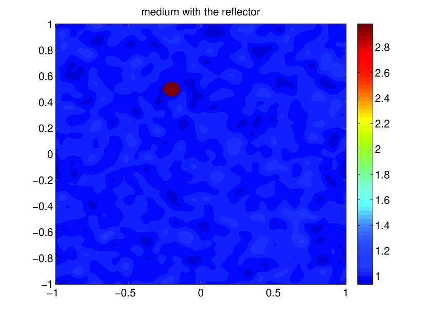
Figure 1: Medium with the reflector.

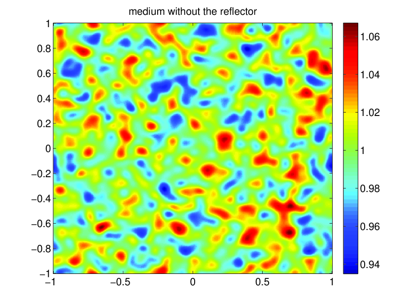
Figure 2: Medium without the reflector (permittivity variations zoomed out).

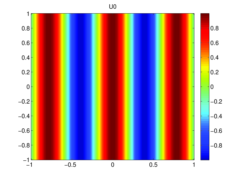
Figure 3: Incoming field $U_{I}$.

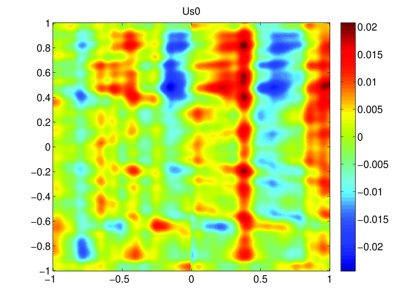
Figure 4: Background field in the absence of a reflector $u_{s}^{(\mu)}$.

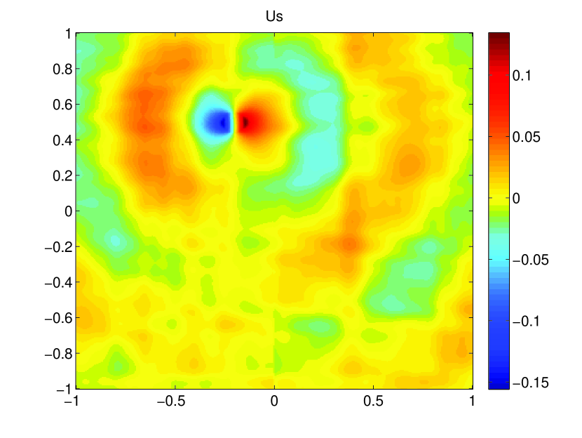
Figure 5: Total scattered field $u_{s}$.

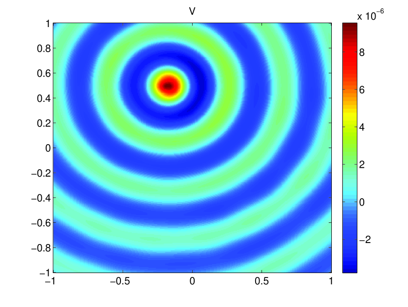
Figure 6: Second-harmonic field $v$.

6.2 The imaging functionals and the effects of the number of plane wave illuminations

We compute the imaging functionals $I$ and $J$ respectively defined in (36) and (39), averaged over four different illuminations settings. We fix the noise level ($\sigma_{\mu}=0,02$), the volume of the particle ($v_{r}=10^{-2}$) and the contrast $\sigma_{r}=2$. In Figures 8 and 8 the image is obtained after backpropagating the boundary data from one illumination ($\theta=0$). On the following graphs, we average over several illumination angles:

• $4$ uniformly distributed angles for Figures 10 and  10.

• $8$ uniformly distributed angles for Figures 12 and  12.

• $32$ uniformly distributed angles for Figures 14 and  14.

As predicted, the shape of the spot on the fundamental frequency imaging is very dependant on the illumination angles, whereas with second-harmonic imaging we get an acceptable image with only one illumination. In applications, averaging over different illumination is useful because it increases the stability with respect to measurement noise. It is noteworthy that, as expected, the resolution of the second-harmonic image is twice higher than the regular imaging one.

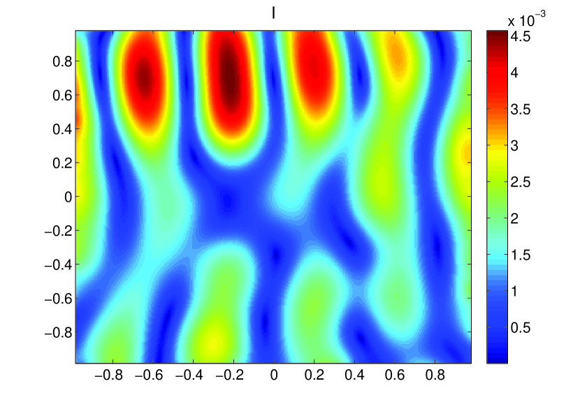
Figure 7: $I$ with $1$ illumination.

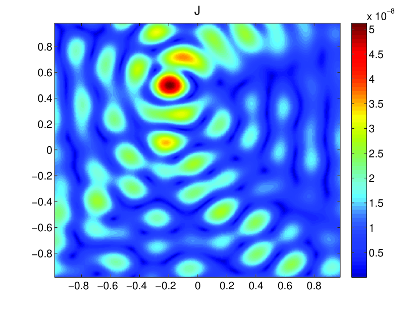
Figure 8: $J$ with $1$ illumination.

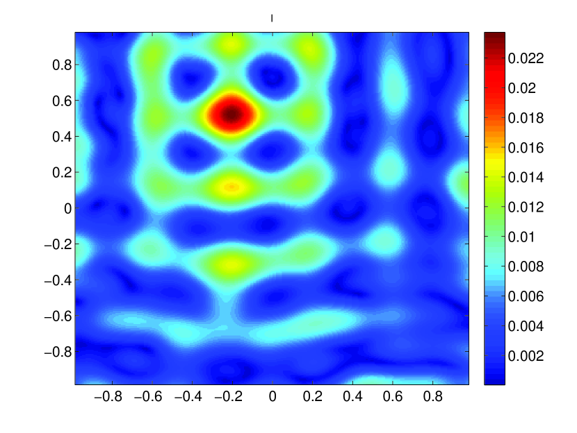
Figure 9: $I$ with $4$ illuminations.

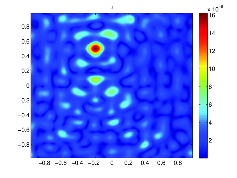
Figure 10: $J$ with $4$ illuminations.

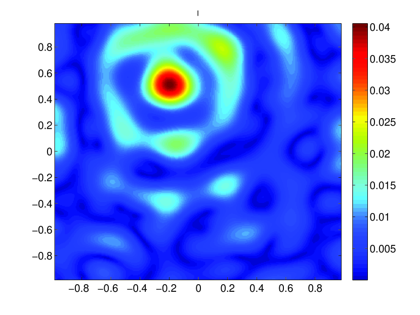
Figure 11: $I$ with $8$ illuminations.

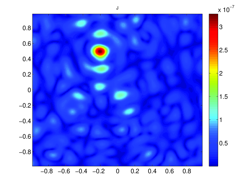
Figure 12: $J$ with $8$ illuminations.

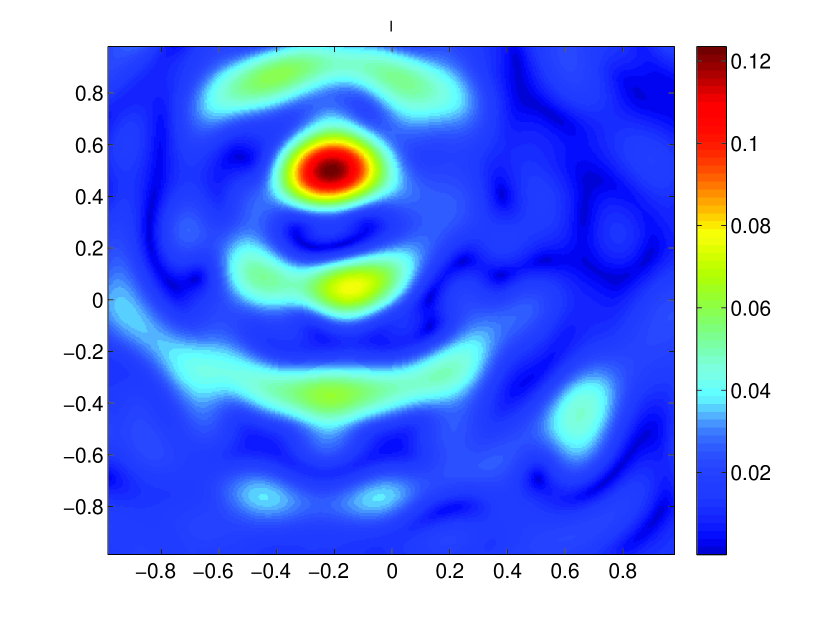
Figure 13: $I$ with $32$ illuminations.

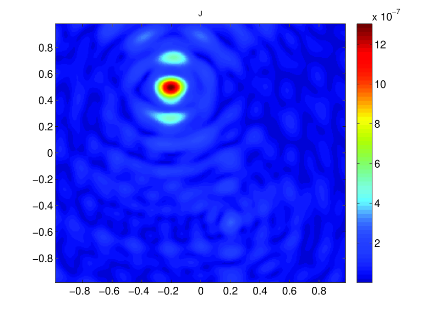
Figure 14: $J$ with $32$ illuminations.

6.3 Statistical analysis

6.3.1 Stability with respect to medium noise

Here we show numerically that the second-harmonic imaging is more stable with respect to medium noise. In Figure 15, we plot the standard deviation of the error $|z_{est}-z_{r}|$ where $z_{est}$ is the estimated location of the reflector. For each level of medium noise we compute the error over $120$ realizations of the medium, using the same parameters, as above. The functional imaging $J$ is clearly more robust than earlier.

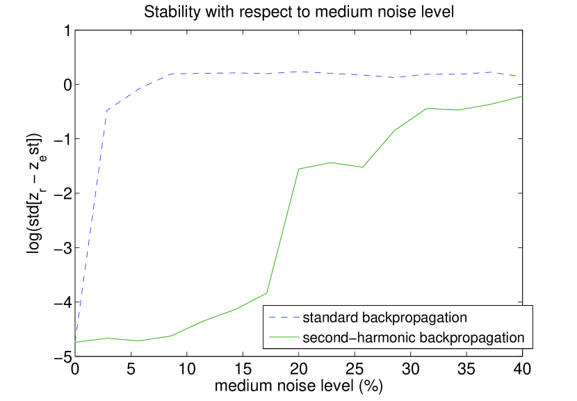
Figure 15: Standard deviation of the localization error with respect to the medium noise level for standard backpropagation (top) and second-harmonic image (bottom).

6.3.2 Effect of the volume of the particle

We show numerically that the quality of the second-harmonic image does not depend on the volume of the particle. We fix the medium noise level ($\sigma_{\mu}=0.02$) and plot the standard deviation of the error with respect to the volume of the particle (Figure 16). We can see that if the particle is too small, the fundamental backpropagation algorithm cannot differentiate the reflector from the medium and the main peak gets buried in the speckle field. The volume of the particle does not have much influence on the second-harmonic image quality.

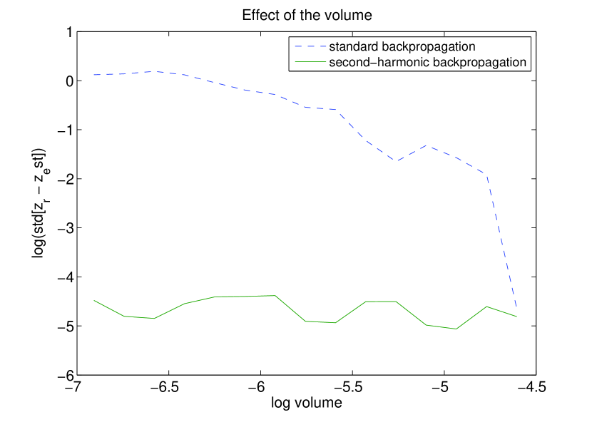
Figure 16: Standard deviation of the localization error with respect to the reflector’s volume (log scale) for standard backpropagation (top) and second-harmonic image (bottom).

6.3.3 Stability with respect to measurement noise

We compute the imaging functionals with a set of data obtained without any medium noise and perturbed with a Gaussian white noise for each of $8$ different illuminations. For each noise level, we average the results over $100$ images. Figure 17 shows that both functionals have similar behaviors.

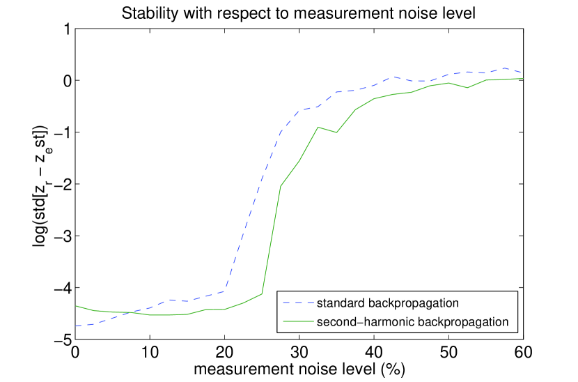
Figure 17: Standard deviation of the localization error with respect to measurement noise level for standard backpropagation (top) and second-harmonic image (bottom).

As mentioned before, in applications, the weakness of the SHG signal will induce a much higher relative measurement noise than in the fundamental data. Since the model we use for measurement noise has a zero expectation, averaging measurements over different illuminations can improve the stability significantly as shown in Figure 18, where the images have been obtained with $16$ illuminations instead of $8$.

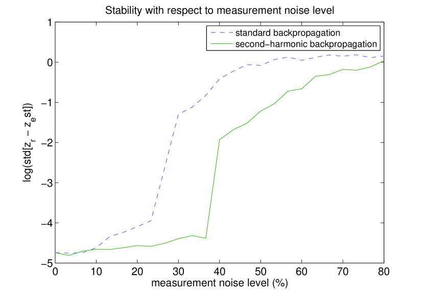
Figure 18: Standard deviation of the localization error with respect to measurement noise level, when averaged over $16$ illuminations of angles uniformly distributed between $0$ and $2\pi$ for standard backpropagation (top) and second-harmonic image (bottom).

7 Concluding remarks

We have studied how second-harmonic imaging can be used to locate a small reflector in a noisy medium, gave asymptotic formulas for the second-harmonic field, and investigated statistically the behavior of the classic and second-harmonic backpropagation functionals. We have proved that the backpropagation algorithm is more stable with respect to medium noise. Our results can also be extended to the case of multiple scatterers as long as they are well-separated.

Appendix A Proof of (8)

Let $R$ be large enough so that $\Omega_{\mu}\Subset B_{R}$, where $B_{R}$ is the ball of radius $R$ and center $0$. Let $S_{R}=\partial B_{R}$ be the sphere of radius $R$, and introduce the Dirichlet-to-Neumann operator $\mathcal{T}$ on $S_{R}$:

$$\mathcal{T}\ :\ H^{1/2}(S_{R}) \longrightarrow H^{-1/2}(S_{R})$$ (149)

$$u \longmapsto\mathcal{T}[u].$$

According to [27], $\mathcal{T}$ is continuous and satisfies

$$-\text{Re }\left<\mathcal{T}[u],u\right>\geq\frac{1}{2R}\|u\|_{L^{2}(S_{R})}^{2},\quad\forall u\in H^{1/2}(S_{R}),$$ (150)

and

$$\text{Im }\left<\mathcal{T}[u],u\right>>0\ \text{if }u\neq 0.$$ (151)

Here, $\left<\,,\,\right>>$ denotes the duality pair between $H^{1/2}(S_{R})$ and $H^{-1/2}(S_{R})$. Now introduce the continuous bilinear form $a$:

$$H^{1}(B_{R})\times H^{1}(B_{R}) \longrightarrow\mathbb{C}$$ (152)

$$(u,v) \longmapsto a(u,v)=\int_{B_{R}}(1+\mu)\nabla u\cdot\overline{\nabla v}-\omega^{2}\int_{B_{R}}u\overline{v}-\left<\mathcal{T}[u],v\right>,$$

as well as the continuous bilinear form $b$:

$$H^{1}(B_{R}) \longrightarrow\mathbb{C}$$ (153)

$$v \longmapsto b(v)=\int_{B_{R}}\mu\nabla U_{0}\cdot\overline{\nabla v}.$$

Problem (5) has the following variational formulation: Find $u\in H^{1}(B_{R})$ such that

$$a(u,v)=b(v)\ \ \forall v\in H^{1}(B_{R}).$$ (154)

With (150) one can show that

$$\text{Re }a(u,u)\geq C_{1}\|\nabla u\|_{L^{2}(B_{R})}^{2}-C_{2}\|u\|_{L^{2}(B_{R})}^{2},$$ (155)

so that $a$ is weakly coercive with respect to the pair $\left(H^{1}(B_{R}),L^{2}(B_{R})\right)$. Since the imbedding of $H^{1}(B_{R})$ into $L^{2}(B_{R})$ is compact we can apply Fredholm’s alternative to problem (154). Hence, we deduce existence of a solution from uniqueness of a solution which easily follows by using identity (151).

Now we want to prove that if $u$ is the solution of (154) then

$$\|u\|_{H^{1}(B_{R})}\leq\|\mu\|_{\infty}.$$ (156)

We proceed by contradiction. Assume that $\forall n\in\mathbb{N}$, there exists $\mu_{n}\in L^{\infty}(B_{R})$ compactly supported and $u_{n}\in H^{1}(B_{R})$ solution of (154) such that

$$\|u_{n}\|_{H^{1}(B_{R})}\geq nC\|\mu_{n}\|_{\infty}.$$ (157)

Consider the sequence:

$$v_{n}=\frac{u_{n}}{\|u_{n}\|_{H^{1}(B_{R})}}.$$ (158)

$(v_{n})_{n\in\mathbb{N}}$ is bounded in $H^{1}(B_{R})$ so there exists a subsequence still denoted by $v_{n}$ and $v^{*}\in H^{1}(B_{R})$ such that $v_{n}\rightharpoonup v^{*}$ in $H^{1}(B_{R})$ and $v_{n}\rightarrow v^{*}$ in $L^{2}(B_{R})$. Now since $u_{n}$ is a solution of (154), we have

$$\int_{B_{R}}(1+\mu_{n})\nabla v_{n}\cdot\overline{\nabla v_{n}}-\omega^{2}\int_{B_{R}}v_{n}\overline{v_{n}}-\left<\mathcal{T}v_{n},v_{n}\right>=\int_{B_{R}}\mu_{n}\nabla U_{0}\cdot\overline{\nabla v_{n}}.$$ (159)

Using (157) we obtain that

$$\int_{B_{R}}(1+\mu_{n})|\nabla v_{n}|^{2}-\omega^{2}\int_{B_{R}}|v_{n}|^{2}-\left<\mathcal{T}v_{n},v_{n}\right>\longrightarrow 0\ (n\rightarrow\infty).$$ (160)

Since $\int_{B_{R}}\mu_{n}|\nabla v_{n}|^{2}\longrightarrow 0$, we get that $\widetilde{a}(v_{n},v_{n})\longrightarrow 0$, where

$$\widetilde{a}(u,v)=\int_{B_{R}}\nabla u\cdot\overline{\nabla v}-\omega^{2}\int_{B_{R}}u\overline{v}-\left<\mathcal{T}u,v\right>.$$ (161)

We want to prove that $v_{n}$ converges strongly in $H^{1}(B_{R})$ to $v^{*}$ and that $v^{*}=0$. This will contradict the fact that $\forall n,\ \|v_{n}\|_{H^{1}(B_{R})}=1$.

Now we decompose $\widetilde{a}=\widetilde{a_{c}}+\widetilde{a_{w}}$ into a coercive part

$$\widetilde{a_{c}}(u,v)=\int_{B_{R}}\nabla u\cdot\overline{\nabla v}-\left<\mathcal{T}u,v\right>$$ (162)

and a weakly continuous part:

$$\widetilde{a_{w}}(u,v)=-\omega^{2}\int_{B_{R}}u\overline{v}.$$ (163)

So $\widetilde{a}(v_{n}-v^{*},v_{n}-v^{*})=\widetilde{a_{c}}(v_{n}-v^{*},v_{n}-v^{*})+\widetilde{a_{w}}(v_{n}-v^{*},v_{n}-v^{*})$. We write $\widetilde{a_{c}}(v_{n}-v^{*},v_{n}-v^{*})=\widetilde{a_{c}}(v_{n}-v^{*})-\widetilde{a_{c}}(v_{n}-v^{*},v^{*})$. Now, since $v_{n}\rightharpoonup v$ in $H^{1}(B_{R})$ and $\widetilde{a_{c}}$ is strongly continuous on $H^{1}(B_{R})^{2}$ we have that $\widetilde{a_{c}}(v_{n}-v^{*},v^{*})\longrightarrow 0$, and $\widetilde{a_{c}}(v_{n}-v^{*},v_{n})=\widetilde{a_{c}}(v_{n},v_{n})-\widetilde{a_{c}}(v^{*},v_{n})\longrightarrow-\widetilde{a_{c}}(v^{*},v^{*})$ which is

$$\widetilde{a_{c}}(v_{n}-v^{*},v_{n}-v^{*})\longrightarrow-\widetilde{a_{c}}(v^{*},v^{*}).$$ (164)

The coercivity of $\widetilde{a_{c}}$ gives

$$\widetilde{a_{c}}(v^{*},v^{*})=0$$ (165)

By a computation similar to the one just above, we also find that

$$\widetilde{a}(v_{n}-v^{*},v_{n}-v^{*})\longrightarrow-\widetilde{a}(v^{*},v^{*}).$$ (166)

Since $\widetilde{a_{w}}(v_{n}-v^{*},v_{n}-v^{*})\longrightarrow 0$, we get that

$$\widetilde{a}(v^{*},v^{*})=0.$$ (167)

So $v^{*}$ =0 and, since $\widetilde{a}$ satisfies (155), we get that $\|\nabla v_{n}\|^{2}_{L^{2}(B_{R})}\longrightarrow 0$ as $n\rightarrow\infty$. We have

$$v_{n}\longrightarrow v=0\text{ in }H^{1}(B_{R}).$$ (168)

Appendix B Proof of Proposition 3.1

Denote $V=u_{s}-u_{s}^{(\mu)}-w^{(\mu)}\cdot\nabla U_{0}(z_{r})$. $V$ is a solution on $\mathbb{R}^{2}$ of

$$\nabla\cdot(1+\mu+[\sigma_{r}-1]\textbf{1}_{\Omega_{r}})\nabla V+\omega^{2}V=-\nabla\cdot[\sigma_{r}-1]\textbf{1}_{\Omega_{r}}\nabla\left[U_{0}-\nabla(x-z_{r})\cdot\nabla U_{0}(z_{r})\right]$$ (169)

subject to the Sommerfeld radiation condition. Now, define $V_{0}$ as the solution on $\mathbb{R}^{2}$ of:

$$\nabla\cdot(1+\mu+[\sigma_{r}-1]\textbf{1}_{\Omega_{r}})\nabla V_{0}=-\nabla\cdot[\sigma_{r}-1]\textbf{1}_{\Omega_{r}}\nabla\left[U_{0}-\nabla(x-z_{r})\cdot\nabla U_{0}(z_{r})\right].$$ (170)

with the condition $V_{0}(x)\longrightarrow 0\ (x\rightarrow\infty)$.

From [5, Lemma A.1], there exist three positive constants $C$, $\widetilde{C}$ and $\kappa$ independent of $\mu$ and $\delta$ such that

$$\|\nabla V_{0}\|_{L^{2}(B_{R})}\leq C\delta\|\nabla\left[U_{0}-\nabla(x-z_{r})\cdot\nabla U_{0}(z_{r})\right]\|_{L^{\infty}(\Omega_{r})},$$ (171)

and

$$\|V_{0}\|_{L^{2}(B_{R})}\leq\widetilde{C}\delta^{1+\kappa}\|\nabla\left[U_{0}-\nabla(x-z_{r})\cdot\nabla U_{0}(z_{r})\right]\|_{L^{\infty}(\Omega_{r})}.$$ (172)

If we write $W=V-V_{0}$, we have that $W$ solves:

$$\nabla\cdot(1+\mu+[\sigma_{r}-1]\textbf{1}_{\Omega_{r}})\nabla W+\omega^{2}W=-\omega^{2}V_{0},$$ (173)

with the boundary condition $\frac{\partial W}{\partial\nu}-\mathcal{T}_{\omega}(W)=\mathcal{T}_{\omega}(V)-\mathcal{T}_{0}(V_{0})$ on $\partial B_{R}$, where $\mathcal{T}_{\omega}$ is the Dirichlet-to-Neumann map on $S_{R}$ defined in (149) associated with the frequency $\omega$. The condition can be re-written : $\frac{\partial W}{\partial\nu}-\mathcal{T}_{\omega}(W)=\left(\mathcal{T}_{\omega}-\mathcal{T}_{0}\right)(V_{0})$. So, based on the well posedness of (173), there exist a constant $C^{\prime}$ independent of $\mu$ and $\delta$ such that

$$\|W\|_{H^{1}(B_{R})}\leq C^{\prime}\left(\|V_{0}\|_{L^{2}(B_{R})}+\|\left[\mathcal{T}_{\omega}-\mathcal{T}_{0}\right](V_{0})\|_{L^{2}(\partial B)}\right).$$ (174)

Now, we can write that, for some constant still denoted $C$ independent of $\mu$ and $\delta$:

$$\|V\|_{H^{1}(B_{R})}\leq C\left(\|V_{0}\|_{H^{1}(B_{R})}+\|V_{0}\|_{L^{2}(B_{R})}\right).$$ (175)

Since $\delta<1$, using (171) and (172) we get

$$\|V\|_{H^{1}(B_{R})}\leq C\delta^{2}.$$ (176)

Appendix C Proof of Proposition 3.3

Denote $\phi$: $y\longrightarrow\widetilde{y}=\phi(y)=\frac{y-z_{r}}{\delta}$. If we define $\forall\widetilde{y}\in B(0,1)$: $\widetilde{w}^{(\mu)}(\widetilde{y})=\frac{1}{\delta}w^{(\mu)}(\phi^{-1}(\widetilde{y}))$, we want to prove the following:

$$\|\widetilde{w}^{(\mu)}(\widetilde{y})-\widetilde{y}-\widetilde{w}(\widetilde{y})\|_{H^{1}(B(0,1))}\leq C\left(\|\mu\|_{\infty}+\delta\omega^{2}\right).$$ (177)

Now, using (11), one can see that $\widetilde{w}^{(\mu)}$ satisfies the following equation:

$$\nabla\cdot\left(1+[\sigma_{r}-1]\mathbf{1}_{B}+\widetilde{\mu}\right)\nabla\widetilde{w}^{(\mu)}+\omega^{2}\delta\widetilde{w}^{(\mu)}=\nabla\cdot\left([\sigma_{r}-1]\mathbf{1}_{B}\nabla\widetilde{y}\right),$$ (178)

where $\widetilde{\mu}=\mu\circ\phi^{-1}$, equipped with the Sommerfeld radiation condition. Using equation (21) we get that

$$\nabla\cdot\left(1+[\sigma_{r}-1]\mathbf{1}_{B}+\widetilde{\mu}\right)\nabla\left(\widetilde{w}^{(\mu)}-\widetilde{y}-\widetilde{w}\right)=-\nabla\cdot\left(\widetilde{\mu}\nabla\widetilde{w}^{(\mu)}\right)-\omega^{2}\delta\widetilde{w}^{(\mu)},$$ (179)

Now, using Meyer’s theorem [25], we get the following estimate:

$$\|\nabla\left(\widetilde{w}^{(\mu)}(\widetilde{y})-\widetilde{y}-\widetilde{w}(\widetilde{y})\right)\|_{L^{2}(B)}\leq C\left(\|\widetilde{\mu}\nabla\widetilde{w}^{(\mu)}\|_{L^{2}(B)}+\omega\delta^{2}\|\widetilde{w}^{(\mu)}\|_{L^{2}(B)}\right).$$ (180)

We need to estimate $\|\widetilde{w}^{(\mu)}\|_{H^{1}(B(0,1))}$. Introduce $\widetilde{w}^{(\mu)}_{0}$ as the solution of

$$\nabla\cdot\left(1+[\sigma_{r}-1]\mathbf{1}_{B}+\widetilde{\mu}\right)\nabla\widetilde{w}^{(\mu)}_{0}=\nabla\cdot\left([\sigma_{r}-1]\mathbf{1}_{B}\nabla\widetilde{y}\right).$$ (181)

with the condition $\widetilde{w}^{(\mu)}_{0}(\widetilde{y})\longrightarrow 0$ as $\widetilde{y}\rightarrow\infty$. Meyers theorem gives:

$$\|\widetilde{w}^{(\mu)}_{0}\|_{H^{1}(B(0,1))}\leq C\|[\sigma_{r}-1]\nabla\widetilde{y}\|_{L^{2}(B(0,1))}.$$ (182)

We can see that $\widetilde{w}^{(\mu)}-\widetilde{w}^{(\mu)}_{0}$ is a solution of

$$\nabla\cdot\left(1+[\sigma_{r}-1]\mathbf{1}_{B}+\widetilde{\mu}\right)\nabla\left(\widetilde{w}^{(\mu)}-\widetilde{w}^{(\mu)}_{0}\right)+\omega^{2}\delta\left(\widetilde{w}^{(\mu)}-\widetilde{w}^{(\mu)}_{0}\right)=-\omega^{2}\delta\widetilde{w}^{(\mu)}_{0}.$$ (183)

We get that

$$\|\widetilde{w}^{(\mu)}-\widetilde{w}^{(\mu)}_{0}\|_{H^{1}(B(0,1))}\leq C\omega^{2}\delta\|\widetilde{w}^{(\mu)}_{0}\|_{L^{2}(B(0,1))}.$$

So, using (182) we get

$$\|\widetilde{w}^{(\mu)}\|_{H^{1}(B(0,1))}\leq C\left(1+\omega^{2}\delta\right).$$ (184)

Since $\|\widetilde{\mu}\nabla\widetilde{w}^{(\mu)}\|_{L^{2}(B(0,1))}\leq\|\widetilde{\mu}\|_{L^{\infty}(B(0,1))}\|\widetilde{w}^{(\mu)}\|_{H^{1}(B(0,1))}$ and $\|\widetilde{\mu}\|_{L^{\infty}(B(0,1))}\leq\|\mu\|_{\infty}$, using (180) and (182) we get

$$\|\nabla\left(\widetilde{w}^{(\mu)}(\widetilde{y})-\widetilde{y}-\widetilde{w}(\widetilde{y})\right)\|_{L^{2}(B(0,1))}\leq C\left(\|\mu\|_{\infty}+\delta\omega^{2}(1+\|\mu\|_{\infty}+\delta\omega^{2})\right),$$

which is exactly, as $\|\mu\|_{\infty}\rightarrow 0$ and $\delta\rightarrow 0$, for $y\in\Omega_{r}$

$$\nabla\left(w^{(\mu)}(y)-(y-z_{r})\right)=\delta\nabla\widetilde{w}(\frac{y-z_{r}}{\delta})+O\left(\delta\|\mu\|_{\infty}+(\delta\omega)^{2}\right).$$ (185)

References

• [1] T. Abboud and H. Ammari. Diffraction at a curved grating: Approximation by an infinite plane grating. J. Math. Anal. Appl., 202:1076–1100, 1996.
• [2] T. Abboud and H. Ammari. Diffraction at a curved grating: Tm and te cases, homogenization. J. Math. Anal. Appl., 202:995–1026, 1996.
• [3] Robert J Adler. The geometry of random fields. Society for Industrial and Applied Mathematics, 2010.
• [4] H. Ammari. An Introduction to Mathematics of Emerging Biomedical Imaging. Springer, 2007.
• [5] H. Ammari, E. Bonnetier, Y. Capdeboscq, M. Tanter, and F. Fink. Electrical impedance tomography by elastic deformation. SIAM J. Appl. Math., 68:1557–1573, 2008.
• [6] H. Ammari, J. Garnier, W. Jing, H. Kang, M. Lim, H. Wang, and K. S$\o$lna. Mathematical and Statistical Methods for Multistatic Imaging. Springer, 2013.
• [7] H. Ammari, J. Garnier, V. Jugnon, and H. Kang. Stability and resolution analysis for a topological derivative based imaging functionnal. SIAM J. Control Optim., 50(1):48–76, 2012.
• [8] H. Ammari and H. Kang. Reconstruction of Small Inhomogeneities from Boundary Measurements. Springer, 2004.
• [9] G. Bao and D.C. Dobson. Second harmonic generation in nonlinear optical films. J. Math. Phys., 35(4):1622–1633, 1994.
• [10] G. Bao, Y. Li, and Z. Zhou. $l^{p}$ estimates of time-harmonic maxwell’s equations in a bounded domain. J. Diff. Equat., 245(12):3674–3686, 2008.
• [11] G. Bao, A. Minut, and Z. Zhou. $l^{p}$ estimates for maxwell’s equations with source term. Comm. Part. Diff. Equat., 32(7-9):1449–1471, 2007.
• [12] A. Bensoussan, J.L. Lions, and G. Papanicolaou. Asymptotic Analysis for Periodic Structures. 1978.
• [13] N. Bloembergen and P.S. Pershan. Light wave at the boundary of nonlinear media. Physical Review, 128(2), October 1962.
• [14] E. Brown and T. McKee. Dynamic imaging of collagen and its modulation in tumors in vivo using second-harmonic generation. Nature medicine, 9(6):796–800, 2003.
• [15] P.J. Campagnola and L.M. Loew. Second-harmonic imaging microscopy for visualizing biomolecular arrays in cells, tissues and organisms. Nature biotechnology, 21(11):1356–1360, 2003.
• [16] M.M. Choy and R.L. Byer. Accurate second-order susceptibility measurements of visible and infrared nonlinear crystals. Physical Review B, 14(4):1693, 1976.
• [17] E. Cuche, F. Bevilacqua, and C. Depeursinge. Digital holography for quantitative phase-contrast imaging. Optics Letters, 24(5):291–293, 1999.
• [18] D. Gilbarg and N.S. Trudinger. Elliptic Partial Differential Equations of Second Order. 1977.
• [19] P. Guyot-Sionnest, W. Chen, and Y.R. Shen. General consideration on optical second-harmonic generation from surfaces and interfaces. Physical Review B, 33(12), June 1986.
• [20] T.F. Heinz. Second-order nonlinear optical effects at surfaces and interfaces. Nonlinear surface electromagnetic phenomena, pages 353–416, 1991.
• [21] C.-L. Hsieh. Imaging with Second-Harmonic Generation Nanoparticles. PhD thesis, California Institute of Technology, 2011.
• [22] C.-L. Hsieh, R. Grange, Y. Pu, and D. Psaltis. Three-dimensional harmonic holographic microcopy using nanoparticles as probes for cell imaging. Optics Express, 17(4):2880–2891, 2009.
• [23] P.M. Hui, C. Xu, and D. Stroud. Second-harmonic generation for a dilute suspension of coated particles. Physical Review B, 69(1):014203, 2004.
• [24] J. Mertz. Nonlinear microscopy: new techniques and applications. Current opinion in neurobiology, 14(5):610–616, 2004.
• [25] N.G. Meyers. An $l^{p}$-estimate for the gradient of solutions of second order elliptic divergence equations. Ann. Scuola Norm. Sup. Pisa, 3:189–206, 1963.
• [26] R.C. Miller. Optical second harmonic generation in piezoelectric crystals. Applied Physics Letters, 5(1):17–19, 1964.
• [27] J. C. Nédélec. Quelques propriétés des dérivées logaritmiques des fonctions de hankel. C.R. Acad. Sci. Paris, 1(314):507–510, 1992.
• [28] Y. Pu, M. Centurion, and D. Psaltis. Harmonic holography: a new holographic principle. Applied Optics, 47(4):A103–A110, 2008.
• [29] U. Schnars and W. Jüptner. Direct recording of holograms by a ccd target and numerical reconstruction. Applied Optics, 33(2):179–181, 1994.
• [30] Y.R. Shen. The Principles of Nonlinear Optics. 1984.
• [31] S. Soussi. Second-harmonic generation in the undepleted-pump approximation. Multiscale Model. Simul., 4(1):115–148, 2005.
• [32] M. Zavelani-Rossi, M. Celebrano, P. Biagioni, D. Polli, M. Finazzi, L. Duò, G. Cerullo, M. Labardi, M. Allegrini, and J. Grand. Near-field second-harmonic generation in single gold nanoparticles. Applied Physics Letters, 92(9):093119–093119, 2008.