Alternative separation of exchange and correlation energies in range-separated density-functional perturbation theory

Abstract

An alternative separation of short-range exchange and correlation energies is used in the framework of second-order range-separated density-functional perturbation theory. This alternative separation was initially proposed by Toulouse et al. [Theor. Chem. Acc. 114, 305 (2005)] and relies on a long-range interacting wavefunction instead of the non-interacting Kohn-Sham one. When second-order corrections to the density are neglected, the energy expression reduces to a range-separated double-hybrid (RSDH) type of functional, RSDHf, where ”f” stands for ”full-range integrals” as the regular full-range interaction appears explicitly in the energy expression when expanded in perturbation theory. In contrast to usual RSDH functionals, RSDHf describes the coupling between long- and short-range correlations as an orbital-dependent contribution. Calculations on the first four noble-gas dimers show that this coupling has a significant effect on the potential energy curves in the equilibrium region, improving the accuracy of binding energies and equilibrium bond distances when second-order perturbation theory is appropriate.

I Introduction

The combination of post-Hartree-Fock (post-HF) methods with density-functional theory (DFT) by means of range separation has been explored in recent years in order to improve the long-range part of standard exchange-correlation functionals. Long-range second-order Møller-Plesset (MP2) Ángyán et al. (2005); Fromager and Jensen (2008); Ángyán (2008); Kullie and Saue (2012), second-order N-electron valence state perturbation theory (NEVPT2) Fromager et al. (2010), Coupled-Cluster (CC) Goll et al. (2005) as well as several long-range variants of the random-phase approximation (RPA) Janesko et al. (2009); Toulouse et al. (2009, 2010) have thus been merged with short-range local and semi-local density-functionals Toulouse et al. (2004, 2004); Goll et al. (2005), and successfully applied to weakly interacting molecular systems Gerber and Ángyán (2007); Zhu et al. (2010); Goll et al. (2005); Liu et al. (2011); Alam and Fromager (2012). Even though such schemes require more computational efforts than standard DFT calculations, they still keep some of the advantages of the latter in terms of basis set convergence and basis set superposition error (BSSE).

In all the range-separated models mentioned previously the complementary short-range density-functional describes not only the purely short-range exchange-correlation energy but also the coupling between long- and short-range correlations Toulouse et al. (2004). Indeed, as the exact short-range exchange energy is obtained from the non-interacting Kohn-Sham (KS) determinant, like in standard DFT, the complementary short-range correlation energy is defined as the difference between the regular full-range correlation density-functional energy and the purely long-range one. Local density approximations (LDA) to the complementary short-range correlation functional can thus be obtained along the same lines as for the regular correlation energy, simply by modeling a uniform electron gas with long-range interactions only Toulouse et al. (2004). Even though range-separated DFT methods for example can describe dispersion forces in noble-gas and alkaline-earth-metal dimers, those based on MP2 or RPA with the long-range HF exchange response kernel (RPAx) often underbind, while a long-range CC treatment can in some cases overbind Toulouse et al. (2010). In order to improve on the description of weak interactions in the equilibrium region, we propose in this work to describe within MP2, not only the purely long-range correlation but also its coupling with the short-range one, while preserving a DFT description of the short-range correlation energy. This can be achieved rigorously when using an alternative separation of the exact short-range exchange and correlation energies that relies on the long-range interacting wave function instead of the KS determinant, as initially proposed by Toulouse et al. Toulouse et al. (2005). The paper is organized as follows: in Sec. II we first motivate the description of the coupling between long- and short-range correlations within MP2 and then briefly present the usual combination of long-range MP2 with short-range DFT, leading thus to the definition of range-separated double hybrid (RSDH) functionals. A new perturbation expansion of the energy is then derived through second order when using the alternative short-range exchange-correlation energy decomposition of Ref. Toulouse et al. (2005). Comparison is then made with conventional double hybrids. The calculation of the orbitals is also discussed. Following the computational details in Sec. III, results obtained for the noble-gas dimers within the short-range local density approximation of Paziani et al. Paziani et al. (2006) are presented. Conclusions are given in Sec. IV.

II Theory

II.1 Range separation of the second-order Møller-Plesset correlation energy

The exact ground-state energy of an electronic system can be expressed as follows

$$E = {\displaystyle\underset{\Psi}{\rm min}\left\{\langle\Psi|\hat{T}+\hat{W}_{\rm ee}+\hat{V}_{\rm ne}|\Psi\rangle\right\}},$$ (1)

where $\hat{T}$ is the kinetic energy operator, $\hat{V}_{\rm ne}$ denotes the nuclear potential operator, and $\hat{W}_{\rm\rm ee}$ is the regular electron-electron interaction. For systems that are not strongly multi-configurational, the exact ground-state wave function that minimizes the energy in Eq. (1) is reasonably well approximated by the HF determinant $\Phi_{0}$ which is obtained when restricting the minimization in Eq. (1) to single determinant wavefunctions. Correlation effects can then be described, for example, in MP perturbation theory where the first-order correction to the wavefunction contains double excitations only, which can be expressed in second-quantized form as Helgaker et al. (2004)

$$|\Psi^{(1)}\rangle=\frac{1}{2}\sum_{ij,ab}t^{ab(1)}_{ij}\hat{E}_{ai}\hat{E}_{bj}|\Phi_{0}\rangle,$$ (2)

where $\hat{E}_{ai}=\hat{a}^{\dagger}_{a,\alpha}\hat{a}_{i,\alpha}+\hat{a}^{\dagger}_{a,\beta}\hat{a}_{i,\beta}$ is a singlet excitation operator while $i,j$ and $a,b$ denote occupied and unoccupied HF orbitals. The MP1 amplitudes are expressed in terms of the HF orbital energies and the two-electron integrals $\langle ab|ij\rangle=\int\int{\rm d}\mathbf{r_{1}}{\rm d}\mathbf{r_{2}}\phi_{a}(\mathbf{r_{1}})\phi_{b}(\mathbf{r_{2}})\frac{1}{r_{12}}\phi_{i}(\mathbf{r_{1}})\phi_{j}(\mathbf{r_{2}})$ as follows

$$t^{ab(1)}_{ij}=\frac{\langle ab|ij\rangle}{\varepsilon_{i}+\varepsilon_{j}-\varepsilon_{a}-\varepsilon_{b}},$$ (3)

and the MP2 correlation energy equals Helgaker et al. (2004)

$$E^{(2)} = \langle\Phi_{0}|\hat{W}_{\rm ee}|\Psi^{(1)}\rangle=\sum_{ij,ab}V^{ij}_{ab}t^{ab(1)}_{ij},$$ (4)

where the two-electron contributions that are contracted with the MP1 amplitudes are expressed as

$$V^{ij}_{ab}=2\langle ab|ij\rangle-\langle ab|ji\rangle.$$ (5)

While the long-range part of the correlation energy can, in many cases, be described reasonably well within MP2, the accurate description of short-range correlation effects usually requires the use of CC methods instead of MP2 which increases the computational cost significantly and requires the use of large atomic basis sets. On the other hand, standard DFT methods enable a rather accurate calculation of the short-range correlation, with a relatively low computational cost, but they fail in describing long-range correlation effects. For that reason, Savin Savin (1996) proposed to separate the two-electron repulsion into short- and long-range parts

$$\frac{1}{r_{12}}=w^{\rm lr,\mu}_{\rm ee}(r_{12})+w^{\rm sr,\mu}_{\rm ee}(r_{12}),$$ (6)

where $\mu$ is a parameter that controls the range separation, so that, for example, a long-range MP2 calculation can be combined rigorously with a short-range DFT one. The commonly used long-range interaction Toulouse et al. (2004) ${w}_{\rm ee}^{\rm lr,\mu}(r_{12})={\rm erf}(\mu r_{12})/r_{12}$, which is considered in this work, is based on the error function but the formalism presented here will be valid for any separation of the two-electron repulsion. While the range separation of the exchange energy is unambiguous, as the latter is linear in the two-electron interaction, the assignment of long- and short-range correlation effects to MP2 and DFT, respectively, is less obvious. Indeed, as both MP1 amplitudes and integrals can be range-separated, according to Eqs. (3), (5) and (6),

$$t^{ab(1)}_{ij} = \Big{(}t^{ab(1)}_{ij}\Big{)}^{\rm lr,\mu}+\Big{(}t^{ab(1)}_{ij}\Big{)}^{\rm sr,\mu},$$

$$V^{ij}_{ab} = \Big{(}V^{ij}_{ab}\Big{)}^{\rm lr,\mu}+\Big{(}V^{ij}_{ab}\Big{)}^{\rm sr,\mu},$$ (7)

the MP2 correlation energy, that is quadratic in the interaction, contains purely long-range and purely short-range contributions as well as long-/short-range coupling terms:

$$\begin{array}[]{l}\displaystyle E^{(2)}=\sum_{ij,ab}\Bigg{[}\Big{(}V^{ij}_{ab}\Big{)}^{\rm lr,\mu}\Big{(}t^{ab(1)}_{ij}\Big{)}^{\rm lr,\mu}+\Big{(}V^{ij}_{ab}\Big{)}^{\rm sr,\mu}\Big{(}t^{ab(1)}_{ij}\Big{)}^{\rm sr,\mu}\\ \\ \hskip 31.2982pt+\Big{(}V^{ij}_{ab}\Big{)}^{\rm lr,\mu}\Big{(}t^{ab(1)}_{ij}\Big{)}^{\rm sr,\mu}+\Big{(}V^{ij}_{ab}\Big{)}^{\rm sr,\mu}\Big{(}t^{ab(1)}_{ij}\Big{)}^{\rm lr,\mu}\Bigg{]}.\end{array}$$ (11)

Since the last two summations on the right-hand side of Eq. (11) are equal,

$$\sum_{ij,ab}\Big{(}V^{ij}_{ab}\Big{)}^{\rm lr,\mu}\Big{(}t^{ab(1)}_{ij}\Big{)}^{\rm sr,\mu}$$ (12)

$$=\sum_{ij,ab}\frac{\big{[}2\langle ab|ij\rangle^{\rm lr,\mu}-\langle ab|ji\rangle^{\rm lr,\mu}\big{]}\langle ab|ij\rangle^{\rm sr,\mu}}{\varepsilon_{i}+\varepsilon_{j}-\varepsilon_{a}-\varepsilon_{b}}$$

$$=\sum_{ij,ab}\frac{2\langle ab|ij\rangle^{\rm sr,\mu}\langle ab|ij\rangle^{\rm lr,\mu}}{\varepsilon_{i}+\varepsilon_{j}-\varepsilon_{a}-\varepsilon_{b}}$$

$$-\sum_{ij,ab}\frac{\langle ab|ij\rangle^{\rm lr,\mu}\langle ab|ji\rangle^{\rm sr,\mu}}{\varepsilon_{j}+\varepsilon_{i}-\varepsilon_{a}-\varepsilon_{b}}$$

$$=\sum_{ij,ab}\Big{(}V^{ij}_{ab}\Big{)}^{\rm sr,\mu}\Big{(}t^{ab(1)}_{ij}\Big{)}^{\rm lr,\mu},$$

the range-separated MP2 correlation energy can finally be rewritten as

$$E^{(2)}=\sum_{ij,ab} \Big{(}V^{ij}_{ab}\Big{)}^{\rm lr,\mu}\Big{(}t^{ab(1)}_{ij}\Big{)}^{\rm lr,\mu}$$ (13)

$$+\Big{(}V^{ij}_{ab}\Big{)}^{\rm sr,\mu}\Big{(}t^{ab(1)}_{ij}\Big{)}^{\rm sr,\mu}$$

$$+2\Big{(}V^{ij}_{ab}\Big{)}^{\rm sr,\mu}\Big{(}t^{ab(1)}_{ij}\Big{)}^{\rm lr,\mu}.$$

In conventional range-separated density-functional perturbation theory Ángyán et al. (2005); Fromager and Jensen (2008); Ángyán (2008), the long-range correlation energy only is described within MP2 while the short-range correlation and its coupling with the long-range one are modeled by a complementary local or semi-local density-functional. While it is important, in terms of computational cost, to describe the purely short-range correlation energy within DFT, the coupling term could in principle be treated within MP2. In the particular case of a van der Waals dimer like Ar₂, for example, this term is not expected to contribute significantly to the dispersion interaction energy at long distance as the short-range integral contributions will vanish. However, in the equilibrium region ($R_{e}\approx 7.1a_{0}$ Tang and Toennies (2003)), the average correlation distance between the valence electrons located on different Ar atoms is approximately $R_{e}-2R_{a}\approx 4.4a_{0}$, where $R_{a}=1.34a_{0}$ is the atomic radius of Ar. The former distance should then be compared with the inverse $1/\mu$ of the range separation parameter that defines qualitatively what are long and short-range interactions Pollet et al. (2002). In conventional range-separated calculations $\mu\approx 0.4-0.5a_{0}^{-1}$ Fromager et al. (2007); Gerber and Ángyán (2005); Kullie and Saue (2012) which leads to $1/\mu\approx 2.0-2.5a_{0}$. As a result, short-range integrals will be of the same order of magnitude or smaller than long-range ones so that, in this case, they can contribute significantly to the dispersion interaction energy. It is thus relevant to raise the question whether an MP2 description of the long-/short-range correlation coupling is not preferable to a DFT one. Note that, as readily seen from Eq. (13), this would only require the computation of the short-range integrals that would then be contracted with the long-range MP1 amplitudes. In this respect, such a new scheme would still be based on a long-range MP2 calculation so that the advantages of the conventional range-separated MP2-DFT model Ángyán et al. (2005) relative to regular MP2, like a faster convergence with respect to the basis set and a smaller BSSE, would be preserved. After a short introduction to conventional range-separated density-functional perturbation theory in Sec. II.2, we will show in Secs. II.3 and II.4 how the long-/short-range MP2 coupling term can be rigorously introduced into the energy expansion through second order by means of a different separation of the exact short-range exchange and correlation energies.

II.2 Range-separated density-functional perturbation theory

In conventional range-separated DFT Savin (1996), which we refer to as short-range DFT (srDFT), the exact ground-state energy is rewritten as

$$E = {\displaystyle\underset{\Psi}{\rm min}\left\{\langle\Psi|\hat{T}+\hat{W}^{\rm lr,\mu}_{\rm ee}+\hat{V}_{\rm ne}|\Psi\rangle+E^{\rm sr,\mu}_{\rm Hxc}[n_{\Psi}]\right\}}$$ (14)

$$= {\displaystyle\langle\Psi^{\mu}|\hat{T}+\hat{W}^{\rm lr,\mu}_{\rm ee}+\hat{V}_{\rm ne}|\Psi^{\mu}\rangle+E^{\rm sr,\mu}_{\rm Hxc}[n_{\Psi^{\mu}}],}$$

where $\hat{W}_{\rm\rm ee}^{\rm lr,\mu}$ is the long-range electron-electron interaction operator. The complementary short-range Hartree-exchange-correlation (srHxc) density-functional energy is denoted $E_{\rm Hxc}^{\rm sr,\mu}[n]$. While Eq. (1) is recovered in the $\mu\rightarrow+\infty$ limit, the other limit $\mu=0$ corresponds to regular KS-DFT as the long-range interaction vanishes and the srHxc functional reduces to the conventional Hxc one. As a zeroth-order approximation, the minimization in Eq. (14) can be performed over single determinant wave functions, leading to the HF-srDFT scheme (referred to as RSH for range-separated hybrid in Ref. Ángyán et al. (2005)). The minimizing HF-srDFT determinant $\Phi_{0}^{\mu}$ fulfills the following long-range HF-type equation

$$\begin{array}[]{l}\hat{H}_{0}|\Phi_{0}^{\mu}\rangle=\mathcal{E}_{0}|\Phi_{0}^{\mu}\rangle,\\ \\ \hat{H}_{0}=\hat{T}+\hat{U}_{\rm HF}^{\rm lr,\mu}+\hat{V}_{\rm ne}+\displaystyle\int{\rm d}{\bf r}\,\dfrac{\delta E_{\rm Hxc}^{\rm sr,\mu}}{\delta n({\bf r})}[n_{\Phi_{0}^{\mu}}]\,\hat{n}({\bf r}),\end{array}$$ (18)

where $\hat{U}_{\rm HF}^{\rm lr,\mu}=\sum_{pq}\sum_{i}\big{(}2\langle pi|qi\rangle^{\rm lr,\mu}-\langle pi|iq\rangle^{\rm lr,\mu}\big{)}\hat{E}_{pq}$ is the long-range analog of the non-local HF potential operator, constructed with the occupied HF-srDFT orbitals, and $\hat{n}({\bf r})$ denotes the density operator. The long-range dynamical correlation effects, which are not described at the HF-srDFT level, can then be treated within a long-range MP-type perturbation theory Goll et al. (2005); Ángyán et al. (2005). For that purpose, we introduce a perturbation strength $\alpha$ and define the auxiliary energy Ángyán et al. (2005)

$$E^{\alpha,\mu}=\underset{\Psi}{\rm min}\Big{\{} \langle\Psi|\hat{T}+(1-\alpha)\hat{U}_{\rm HF}^{\rm lr,\mu}+\alpha\hat{W}_{\rm ee}^{\rm lr,\mu}|\Psi\rangle$$ (19)

$$+\langle\Psi|\hat{V}_{\rm ne}|\Psi\rangle+E^{\rm sr,\mu}_{\rm Hxc}[n_{\Psi}]\Big{\}}.$$

The minimizing wave function $\Psi^{\alpha,\mu}$ in Eq. (19) can be obtained self-consistently from the following non-linear eigenvalue-type equation

$$\begin{array}[]{l}\Bigg{(}\hat{T}+(1-\alpha)\hat{U}_{\rm HF}^{\rm lr,\mu}+\alpha\hat{W}_{\rm ee}^{\rm lr,\mu}+\hat{V}_{\rm ne}\\ \\ +\displaystyle\int{\rm d}{\bf r}\,\dfrac{\delta E_{\rm Hxc}^{\rm sr,\mu}}{\delta n({\bf r})}[n_{\Psi^{\alpha,\mu}}]\,\hat{n}({\bf r})\Bigg{)}|\Psi^{\alpha,\mu}\rangle=\mathcal{E}^{\alpha,\mu}|\Psi^{\alpha,\mu}\rangle.\end{array}$$ (23)

It is readily seen, from Eqs. (18) and (23), that in the $\alpha=0$ limit, $\Psi^{\alpha,\mu}$ reduces to the HF-srDFT determinant $\Phi_{0}^{\mu}$, while, according to Eqs. (14) and (19), the auxiliary energy becomes, for $\alpha=1$, the exact ground-state energy and $\Psi^{\alpha,\mu}$ reduces to the minimizing wave function $\Psi^{\mu}$ in Eq. (14). Using the intermediate normalization condition

$$\langle\Phi_{0}^{\mu}|\Psi^{\alpha,\mu}\rangle=1,\hskip 14.22636pt0\leq\alpha\leq 1,$$ (24)

it was shown Ángyán et al. (2005); Fromager and Jensen (2008); Ángyán (2008); Fromager and Jensen (2011) that the wave function can be expanded through second order as follows

$$|\Psi^{\alpha,\mu}\rangle = |\Phi_{0}^{\mu}\rangle+\alpha|\Psi^{\rm(1)lr,\mu}\rangle+\alpha^{2}|\Psi^{\rm(2)\mu}\rangle+\mathcal{O}(\alpha^{3}),$$ (25)

where the first-order contribution is the long-range analog of the MP1 wavefunction correction

$$|\Psi^{(1)\rm lr,\mu}\rangle=\frac{1}{2}\sum_{ij,ab}\Big{(}t^{ab(1)}_{ij}\Big{)}^{\rm lr,\mu}\hat{E}_{ai}\hat{E}_{bj}|\Phi^{\mu}_{0}\rangle,$$ (26)

that is computed with HF-srDFT orbitals and orbital energies. Indeed, according to the Brillouin theorem, the density remains unchanged through first order, leading to the following Taylor expansion, through second order, for the density:

$$n_{\Psi^{\alpha,\mu}}({\bf r}) = n_{\Phi^{\mu}_{0}}({\bf r})+\alpha^{2}\delta n^{(2)\mu}({\bf r})+\mathcal{O}(\alpha^{3}),$$ (27)

so that self-consistency effects in Eq. (23) do not contribute to the wave function through first order. Non-zero contributions actually appear through second order in the wave function Fromager and Jensen (2011). Finally, the auxiliary energy can be expanded as Ángyán et al. (2005); Fromager and Jensen (2008)

$$\begin{array}[]{l}\displaystyle{E}^{\alpha,\mu}={E}^{(0)\mu}+\alpha{E}^{(1)\mu}+\alpha^{2}{E}^{(2)\mu}+\mathcal{O}(\alpha^{3}),\end{array}$$ (29)

where, when considering the $\alpha=1$ limit, the HF-srDFT energy is recovered through first order

$$E_{\rm\tiny HF}^{\rm\tiny srDFT} = {E}^{(0)\mu}+{E}^{(1)\mu}$$

$$= \langle\Phi_{0}^{\mu}|\hat{T}+\hat{W}_{\rm ee}^{\rm lr,\mu}+\hat{V}_{\rm ne}|\Phi_{0}^{\mu}\rangle+E_{\rm Hxc}^{\rm sr,\mu}[n_{\Phi_{0}^{\mu}}],$$

and the second-order correction to the energy is the purely long-range MP2 correlation energy

$$E^{(2)\mu}=\sum_{ij,ab} \Big{(}V^{ij}_{ab}\Big{)}^{\rm lr,\mu}\Big{(}t^{ab(1)}_{ij}\Big{)}^{\rm lr,\mu}.$$ (31)

In summary, the HF-srDFT scheme defines an approximate one-parameter RSH exchange-correlation energy which combines exact long-range exchange with complementary srDFT exchange-correlation energies:

$$E_{\rm xc,RSH}^{\rm\mu} = -\sum_{ij}\langle ij|ji\rangle^{\rm lr,\mu}+E_{\rm x}^{\rm sr,\mu}[n_{\Phi_{0}^{\mu}}]$$ (32)

$$+E_{\rm c}^{\rm sr,\mu}[n_{\Phi_{0}^{\mu}}].$$

Including second-order terms leads to the MP2-srDFT energy expression Fromager and Jensen (2008) (referred to as RSH+MP2 in Ref. Ángyán et al. (2005)),

$$E_{\rm\tiny MP2}^{\rm\tiny srDFT} = E_{\rm\tiny HF}^{\rm\tiny srDFT}+E^{(2)\mu},$$ (33)

which defines, according to Eq. (31), an approximate one-parameter range-separated double hybrid exchange-correlation energy expression

$$E_{\rm xc,RSDH}^{\rm\mu} = -\sum_{ij}\langle ij|ji\rangle^{\rm lr,\mu}+\sum_{ij,ab}\Big{(}V^{ij}_{ab}\Big{)}^{\rm lr,\mu}\Big{(}t^{ab(1)}_{ij}\Big{)}^{\rm lr,\mu}$$ (34)

$$+E_{\rm x}^{\rm sr,\mu}[n_{\Phi_{0}^{\mu}}]+E_{\rm c}^{\rm sr,\mu}[n_{\Phi_{0}^{\mu}}],$$

where both the purely short-range correlation energy and its coupling with the long-range one are described by the complementary short-range correlation density-functional.

II.3 Alternative decomposition of the short-range exchange-correlation energy

Since the exact short-range exchange-correlation density-functional is unknown, local and semi-local approximations have been developed in order to perform practical srDFT calculations Savin (1996); Toulouse et al. (2004); Heyd et al. (2003); Heyd and Scuseria (2004); Toulouse et al. (2004); Gori-Giorgi and Savin (2006); Goll et al. (2005, 2009). The former are based on the following decomposition of the srHxc energy

$$E_{\rm Hxc}^{\rm sr,\mu}[n] = E_{\rm H}^{\rm sr,\mu}[n]+E_{\rm x}^{\rm sr,\mu}[n]+E_{\rm c}^{\rm sr,\mu}[n],$$ (35)

$$E_{\rm H}^{\rm sr,\mu}[n] = \frac{1}{2}\int\int{\rm d}{\mathbf{r}}\,{\rm d}{\mathbf{r^{\prime}}}\,n(\mathbf{r})\,n(\mathbf{r^{\prime}})\,w_{\rm ee}^{\rm sr,\mu}\left(|{\bf r}-{\bf r^{\prime}}|\right),$$

$$E_{\rm x}^{\rm sr,\mu}[n] = \langle\Phi^{\rm KS}[n]|\hat{W}_{\rm ee}^{\rm sr,\mu}|\Phi^{\rm KS}[n]\rangle-E_{\rm H}^{\rm sr,\mu}[n],$$

where the short-range correlation energy is defined with respect to the KS determinant $\Phi^{\rm KS}[n]$ like in standard DFT. As an alternative, Toulouse, Gori-Giorgi and Savin Toulouse et al. (2005); Gori-Giorgi and Savin (2009) proposed a decomposition which relies on the ground state $\Psi^{\rm\mu}[n]$ of the long-range interacting system whose density equals $n$:

$$E_{\rm Hxc}^{\rm sr,\mu}[n] = \langle\Psi^{\rm\mu}[n]|\hat{W}_{\rm ee}^{\rm sr,\mu}|\Psi^{\rm\mu}[n]\rangle+E_{\rm\rm c,md}^{\rm sr,\mu}[n].$$ (36)

The first term in the right-hand side of Eq. (36) was referred to as ”multideterminantal” (”md”) short-range exact exchange Gori-Giorgi and Savin (2009). As shown in the following, it contains not only the short-range exchange energy but also coupling terms between long- and short-range correlations. Note that, according to Eq. (36), the complementary ”md” short-range correlation functional differs from the conventional one defined in Eq. (35):

$$E_{\rm\rm c,md}^{\rm sr,\mu}[n] = E_{\rm\rm c}^{\rm sr,\mu}[n]+\langle\Phi^{\rm KS}[n]|\hat{W}_{\rm ee}^{\rm sr,\mu}|\Phi^{\rm KS}[n]\rangle$$ (37)

$$-\langle\Psi^{\rm\mu}[n]|\hat{W}_{\rm ee}^{\rm sr,\mu}|\Psi^{\rm\mu}[n]\rangle.$$

This expression has been used in Refs. Toulouse et al. (2005); Paziani et al. (2006) for developing short-range ”md” LDA correlation functionals. Returning to the exact energy expression in Eq. (14), the srHxc energy can be written as

$$E_{\rm Hxc}^{\rm sr,\mu}[n_{\Psi^{\mu}}] = \langle\Psi^{\rm\mu}|\hat{W}_{\rm ee}^{\rm sr,\mu}|\Psi^{\rm\mu}\rangle+E_{\rm c,md}^{\rm sr,\mu}[n_{\Psi^{\mu}}],$$ (38)

using the decomposition in Eq. (36) and the first Hohenberg–Kohn theorem Hohenberg and Kohn (1964) which ensures, according to Eq. (23) in the $\alpha=1$ limit, that $\Psi^{\mu}$ is the ground state of a long-range interacting system and therefore

$$\Psi^{\mu}[n_{\Psi^{\mu}}] = \Psi^{\mu}.$$ (39)

When adding long- and short-range interactions in Eq. (14), the exact ground-state energy expression becomes Toulouse et al. (2005)

$$E = \langle\Psi^{\mu}|\hat{T}+\hat{W}_{\rm ee}+\hat{V}_{\rm ne}|\Psi^{\mu}\rangle+E_{\rm c,md}^{\rm sr,\mu}[n_{\Psi^{\mu}}].$$ (40)

As shown in Sec. II.4, using such an expression, in combination with the MP2-srDFT perturbation expansion of the wave function in Eq. (25), will enable us to define a new class of RSDH functionals where both the purely long-range MP2 correlation energy and the long-/short-range MP2 coupling term appear explicitly in the energy expansion through second order. Let us finally mention that, as shown by Sharkas et al. Sharkas et al. (2011), regular double hybrid density-functional energy expressions can be derived when considering a scaled interaction $\lambda_{1}/r_{12}$ instead of a long-range one based on the error function. With the notations of Ref. Fromager (2011) , the short-range exchange-correlation energy decomposition in Eq. (36) becomes, for the scaled interaction,

$$\overline{E}^{\lambda_{1}}_{\rm Hxc}[n]=(1-\lambda_{1})\langle\Psi^{\lambda_{1}}[n]|\hat{W}_{\rm ee}|\Psi^{\lambda_{1}}[n]\rangle+\overline{E}^{\lambda_{1}}_{\rm c,md}[n],$$ (41)

where $\Psi^{\lambda_{1}}[n]$ is the ground state of the $\lambda_{1}$-interacting system whose density equals $n$. As further discussed in Sec. II.5, the new class of RSDH which is derived in this work can be connected to conventional two-parameter double hybrids by means of Eq. (41).

II.4 New class of range-separated double hybrid density-functionals

In order to derive a new perturbation expansion of the energy based on Eq. (40), we introduce a modified auxiliary energy

$$\begin{array}[]{l}\displaystyle\tilde{E}^{\alpha,\mu}={E}^{\alpha,\mu}-E_{\rm Hxc}^{\rm sr,\mu}[n_{\Psi^{\alpha,\mu}}]\\ \\ \hskip 36.98866pt+\alpha\dfrac{\langle\Psi^{\alpha,\mu}|\hat{W}_{\rm ee}^{\rm sr,\mu}|\Psi^{\alpha,\mu}\rangle}{\langle\Psi^{\alpha,\mu}|\Psi^{\alpha,\mu}\rangle}+E_{\rm c,md}^{\rm sr,\mu}[n_{\Psi^{\alpha,\mu}}],\end{array}$$ (45)

which reduces, like ${E}^{\alpha,\mu}$, to the exact ground-state energy in the $\alpha=1$ limit. As argued in Sec. II.1, RSDH functionals are well adapted to the description of weakly interacting systems. We also pointed out that, for standard $\mu$ values, the short-range integrals associated to dispersion interactions may be of the same order of magnitude or smaller than their long-range counterparts. It is therefore relevant, for such systems, to consider the short-range interaction as a first-order contribution in perturbation theory, like the long-range fluctuation operator in MP2-srDFT (see Eq. (19)). This justifies the multiplication by $\alpha$ of the short-range interaction expectation value in Eq. (45). It also ensures that truncating the Taylor expansion of the modified auxiliary energy through second order is as relevant as for the auxiliary energy used in MP2-srDFT. Let us mention that the perturbation theory presented in the following differs from MP2-srDFT only by the energy expansion. Both approaches will indeed be based on the same wavefunction perturbation expansion. As discussed further in Sec. II.6, it is, in principle, possible to correct both the wave function and the energy consistently when combining optimized effective potential (OEP) techniques with range separation. Note also, in Eq. (45), the normalization factor in front of the short-range interaction expectation value, which must be introduced since the intermediate normalization is used (see Eq. (24)). From the wavefunction perturbation expansion in Eq. (25), we thus obtain the orthogonality condition $\langle\Phi^{\mu}_{0}|\Psi^{\rm(1)lr,\mu}\rangle=0$ and, as a result, the following Taylor expansion:

$$\begin{array}[]{l}\displaystyle\frac{\left\langle\Psi^{\alpha,\mu}\right|\hat{W}_{\rm ee}^{\rm sr,\mu}\left|\Psi^{\alpha,\mu}\right\rangle}{\langle\Psi^{\alpha,\mu}|\Psi^{\alpha,\mu}\rangle}=\left\langle\Phi^{\mu}_{0}\right|\hat{W}_{\rm ee}^{\rm sr,\mu}\left|\Phi^{\mu}_{0}\right\rangle\\ \\ +2\alpha\langle\Phi^{\mu}_{0}|\hat{W}_{\rm ee}^{\rm sr,\mu}|\Psi^{\rm(1)lr,\mu}\rangle+\mathcal{O}(\alpha^{2}).\end{array}$$ (49)

In addition, according to Eq. (27), the short-range density-functional energy difference can be expanded through second order as

$$\begin{array}[]{l}\Big{(}E_{\rm c,md}^{\rm sr,\mu}-E_{\rm Hxc}^{\rm sr,\mu}\Big{)}[n_{\Psi^{\alpha,\mu}}]=\Big{(}E_{\rm c,md}^{\rm sr,\mu}-E_{\rm Hxc}^{\rm sr,\mu}\Big{)}[n_{\Phi_{0}^{\mu}}]\\ \\ \displaystyle+\alpha^{2}\int{\rm d}{\bf r}\,\Bigg{(}\dfrac{\delta E_{\rm c,md}^{\rm sr,\mu}}{\delta n({\bf r})}-\dfrac{\delta E_{\rm Hxc}^{\rm sr,\mu}}{\delta n({\bf r})}\Bigg{)}[n_{\Phi_{0}^{\mu}}]\;\delta n^{(2)\mu}({\bf r})\\ \\ +\mathcal{O}(\alpha^{3}).\end{array}$$ (55)

As a result, we obtain from Eqs. (29), (45), (49) and (55) a new Taylor expansion for the energy

$$\begin{array}[]{l}\displaystyle\tilde{E}^{\alpha,\mu}=\tilde{E}^{(0)\mu}+\alpha\tilde{E}^{(1)\mu}+\alpha^{2}\tilde{E}^{(2)\mu}+\mathcal{O}(\alpha^{3}),\end{array}$$ (57)

where

$$\begin{array}[]{l}\tilde{E}^{(0)\mu}={E}^{(0)\mu}+\Big{(}E_{\rm c,md}^{\rm sr,\mu}-E_{\rm Hxc}^{\rm sr,\mu}\Big{)}[n_{\Phi_{0}^{\mu}}],\\ \\ \tilde{E}^{(1)\mu}={E}^{(1)\mu}+{\langle\Phi_{0}^{\mu}|\hat{W}_{\rm ee}^{\rm sr,\mu}|\Phi_{0}^{\mu}\rangle},\\ \\ \tilde{E}^{(2)\mu}={E}^{(2)\mu}+2{\langle\Phi_{0}^{\mu}|\hat{W}_{\rm ee}^{\rm sr,\mu}|\Psi^{(1)\rm lr,\mu}\rangle}\\ \\ \displaystyle+\int{\rm d}{\bf r}\,\Bigg{(}\dfrac{\delta E_{\rm c,md}^{\rm sr,\mu}}{\delta n({\bf r})}-\dfrac{\delta E_{\rm Hxc}^{\rm sr,\mu}}{\delta n({\bf r})}\Bigg{)}[n_{\Phi_{0}^{\mu}}]\;\delta n^{(2)\mu}({\bf r}).\\ \end{array}$$ (65)

According to Eq. (II.2), in the $\alpha=1$ limit, we recover through first order what can be referred to as a RSH energy expression with full-range integrals (RSHf)

$${E}_{\rm RSHf} = \tilde{E}^{(0)\mu}+\tilde{E}^{(1)\mu}$$

$$= \langle\Phi_{0}^{\mu}|\hat{T}+\hat{W}_{\rm ee}+\hat{V}_{\rm ne}|\Phi_{0}^{\mu}\rangle+E_{\rm c,md}^{\rm sr,\mu}[n_{\Phi_{0}^{\mu}}],$$

which defines the approximate one-parameter RSHf exchange-correlation energy

$$E_{\rm xc,RSHf}^{\rm\mu} = -\sum_{ij}\langle ij|ji\rangle+E_{\rm c,md}^{\rm sr,\mu}[n_{\Phi_{0}^{\mu}}].$$ (67)

Turning to the second-order energy corrections in Eq. (65), the second term on the right-hand side of the third equation can be identified, by analogy with Eq. (4), as the long-/short-range MP2 coupling term that was introduced in the range-separated expression of the MP2 correlation energy in Eq. (13):

$$2\langle\Phi^{\mu}_{0}|\hat{W}_{\rm ee}^{\rm sr,\mu}|\Psi^{\rm(1)lr,\mu}\rangle = 2\sum_{ij,ab}\Big{(}V^{ij}_{ab}\Big{)}^{\rm sr,\mu}\Big{(}t^{ab(1)}_{ij}\Big{)}^{\rm lr,\mu}.$$ (68)

Note that this coupling is here expressed in terms of the HF-srDFT orbitals and orbital energies. We thus deduce from Eq. (31) the final expression for the second-order correction to the energy:

$$\begin{array}[]{l}\displaystyle\tilde{E}^{(2)\mu}=\sum_{ij,ab}\Bigg{[}\Big{(}V^{ij}_{ab}\Big{)}^{\rm lr,\mu}+2\Big{(}V^{ij}_{ab}\Big{)}^{\rm sr,\mu}\Bigg{]}\Big{(}t^{ab(1)}_{ij}\Big{)}^{\rm lr,\mu}\\ \\ \displaystyle+\int{\rm d}{\bf r}\,\Bigg{(}\dfrac{\delta E_{\rm c,md}^{\rm sr,\mu}}{\delta n({\bf r})}-\dfrac{\delta E_{\rm Hxc}^{\rm sr,\mu}}{\delta n({\bf r})}\Bigg{)}[n_{\Phi_{0}^{\mu}}]\;\delta n^{(2)\mu}({\bf r}).\end{array}$$ (72)

Note that Eqs. (II.4) and  (72) provide an energy expression which is exact through second order. Note also that, in contrast to MP2-srDFT Ángyán (2008, 2009) for which the auxiliary energy in Eq. (19) has a variational expression, the $2n+1$ rule is not fulfilled here as the modified auxiliary energy expression in Eq. (45) is not variational. In other words, the Hellmann–Feynman theorem does not hold in this context. If we neglect the second-order correction to the density, that is well justified for molecular systems which are not multi-configurational Fromager and Jensen (2011); Goll et al. (2005), we obtain a RSDH energy expression involving, through the exchange energy, full-range integrals (RSDHf)

$$\begin{array}[]{l}{E}_{\rm RSDHf}={E}_{\rm RSHf}\\ \displaystyle+\sum_{ij,ab}\Bigg{[}\Big{(}V^{ij}_{ab}\Big{)}^{\rm lr,\mu}+2\Big{(}V^{ij}_{ab}\Big{)}^{\rm sr,\mu}\Bigg{]}\Big{(}t^{ab(1)}_{ij}\Big{)}^{\rm lr,\mu}.\end{array}$$ (75)

Note that, according to Eqs. (31), (33) and (75), the same long-range correlation energy expression, that is based on MP2, is used in both RSDHf and MP2-srDFT schemes. The former differs from the latter, in the second-order correlation energy correction, only by the coupling between long- and short-range correlations that is now described within MP2,

$${E}_{\rm RSDHf}-E_{\rm\tiny MP2}^{\rm\tiny srDFT} = {E}_{\rm RSHf}+2\sum_{ij,ab}\Big{(}V^{ij}_{ab}\Big{)}^{\rm sr,\mu}\Big{(}t^{ab(1)}_{ij}\Big{)}^{\rm lr,\mu}$$ (76)

$$-E_{\rm\tiny HF}^{\rm\tiny srDFT}.$$

Hence, according to Eq. (67), the RSDHf energy expression in Eq. (75) defines a new type of approximate one-parameter RSDH exchange-correlation energy,

$$\begin{array}[]{l}E_{\rm xc,RSDHf}^{\mu}=\displaystyle-\sum_{ij}\langle ij|ji\rangle\\ \displaystyle+\sum_{ij,ab}\Bigg{[}\Big{(}V^{ij}_{ab}\Big{)}^{\rm lr,\mu}+2\Big{(}V^{ij}_{ab}\Big{)}^{\rm sr,\mu}\Bigg{]}\Big{(}t^{ab(1)}_{ij}\Big{)}^{\rm lr,\mu}\\ \\ +E_{\rm c,md}^{\rm sr,\mu}[n_{\Phi_{0}^{\mu}}],\end{array}$$ (81)

which is, in addition, self-interaction free as both long- and short-range exchange energies are treated exactly. In conclusion, according to Eqs. (34) and (81), RSDHf differ from MP2-srDFT in terms of exchange and correlation energies as follows:

$$E_{\rm x,RSDHf}^{\mu}-E_{\rm x,RSDH}^{\mu} = -\sum_{ij}\langle ij|ji\rangle^{\rm sr,\mu}-E_{\rm x}^{\rm sr,\mu}[n_{\Phi_{0}^{\mu}}],$$

$$E_{\rm c,RSDHf}^{\mu}-E_{\rm c,RSDH}^{\mu} = E_{\rm c,md}^{\rm sr,\mu}[n_{\Phi_{0}^{\mu}}]$$ (82)

$$+2\sum_{ij,ab}\Big{(}V^{ij}_{ab}\Big{)}^{\rm sr,\mu}\Big{(}t^{ab(1)}_{ij}\Big{)}^{\rm lr,\mu}$$

$$-E_{\rm c}^{\rm sr,\mu}[n_{\Phi_{0}^{\mu}}].$$

It is known that, in practice, standard hybrid functionals only use a fraction of exact exchange. The situation here is quite different as a part of the correlation energy is treated explicitly in perturbation theory. In this respect, it is not irrelevant to investigate RSDH schemes that use $100\%$ of full-range exact exchange. Numerical results presented in Sec. IV actually support this statement. Nevertheless, as shown in Appendix A, a two-parameter RSDHf (2RSDHf) model can be formulated when introducing a fraction $\lambda$ of exact short-range exchange energy. This leads to the following exchange-correlation expression

$$E_{\rm xc,2RSDHf}^{\mu,\lambda} = -\sum_{ij}\Big{[}\langle ij|ji\rangle^{\rm lr,\mu}+\lambda\langle ij|ji\rangle^{\rm sr,\mu}\Big{]}$$ (83)

$$+\sum_{ij,ab}\Bigg{[}\Big{(}V^{ij}_{ab}\Big{)}^{\rm lr,\mu}+2\lambda\Big{(}V^{ij}_{ab}\Big{)}^{\rm sr,\mu}\Bigg{]}\Big{(}t^{ab(1)}_{ij}\Big{)}^{\rm lr,\mu}$$

$$+(1-\lambda)\Big{(}{E}_{\rm\rm x}^{\rm sr,\mu}[n_{\Phi_{0}^{\mu}}]+{E}_{\rm\rm c}^{\rm sr,\mu}[n_{\Phi_{0}^{\mu}}]\Big{)}$$

$$+\lambda E_{\rm c,md}^{\rm sr,\mu}[n_{\Phi_{0}^{\mu}}].$$

As readily seen in Eq. (83), the 2RSDHf scheme reduces to MP2-srDFT and RSDHf models in the $\lambda=0$ and $\lambda=1$ limits, respectively. Note that, for any value of $\lambda$, the long-range exchange and purely long-range correlation energies are fully treated at the HF and MP2 levels, respectively. As a result, the second parameter $\lambda$ can only be used for possibly improving, in practice, the description of the complementary short-range energy. Such a scheme is not further investigated in this paper and is left for future work.

II.5 Connection with conventional double hybrids

As shown in Refs. Fromager (2011); Cornaton et al. (2013), the exchange-correlation energy expression that is used in conventional two-parameter double hybrids (2DH),

$$\begin{array}[]{l}\displaystyle E_{\rm{xc},\mbox{\tiny 2DH}}^{a_{\rm x},a_{\rm c}}=-a_{\rm x}\sum_{ij}\langle ij|ji\rangle+(1-a_{\rm x})E_{\rm x}[n]\\ \displaystyle\hskip 45.52458pt+(1-a_{\rm c})E_{\rm c}[n]+a_{\rm c}\sum_{ij,ab}V^{ij}_{ab}t^{ab(1)}_{ij},\end{array}$$ (86)

can be derived within density-functional perturbation theory when the following conditions are fulfilled:

$$0\leq a_{\rm x} \leq 1,$$

$$0\leq a_{\rm c} \leq a^{2}_{\rm x}.$$ (87)

This is achieved when applying the MP2 approach to an electronic system whose interaction is scaled as $\lambda_{1}/r_{12}$ where

$$\begin{array}[]{l}\lambda_{1}=a_{\rm x}-\sqrt{a^{2}_{\rm x}-a_{\rm c}}.\end{array}$$ (89)

As already mentioned in Sec. II.3, an analogy can be made between regular double hybrids and the RSDHf model derived in Sec. II.4, considering first, according to Eq. (81), a fraction of 100% for the exact exchange energy

$$a_{\rm x} = 1,$$ (90)

which, according to Eq. (89), leads to

$$a_{\rm c}=1-(1-\lambda_{1})^{2}.$$ (91)

When switching from the scaled to the long-range interaction,

$$\lambda_{1}/r_{12}\;\rightarrow\;w^{\rm lr,\mu}_{\rm ee}(r_{12}),$$ (92)

or equivalently

$$(1-\lambda_{1})/r_{12}\;\rightarrow\;w^{\rm sr,\mu}_{\rm ee}(r_{12}),$$ (93)

the fraction of MP2 correlation energy in a regular double hybrid becomes, according to Eqs. (91) and (93),

$$a_{\rm c}\sum_{ij,ab}V^{ij}_{ab}t^{ab(1)}_{ij} \;\rightarrow\; \sum_{ij,ab}V^{ij}_{ab}t^{ab(1)}_{ij}$$ (94)

$$-\sum_{ij,ab}\Big{(}V^{ij}_{ab}\Big{)}^{\rm sr,\mu}\Big{(}t^{ab(1)}_{ij}\Big{)}^{\rm sr,\mu},$$

and, from Eq. (41) as well as Eqs. (10), (13) and (36) in Ref. Fromager (2011), we obtain for the DFT correlation term

$$(1-a_{\rm c})E_{\rm c}[n]\approx\overline{E}^{\lambda_{1}}_{\rm c,md}[n] \;\rightarrow\; E_{\rm c,md}^{\rm sr,\mu}[n],$$ (95)

where, on the left-hand side of Eq. (LABEL:corr_ener_connection_2blehybrid_dft), the uniform coordinate scaling in the density has been neglected, as in conventional double hybrids Sharkas et al. (2011); Fromager (2011). As a result, using Eqs. (4) and (13), we recover by simple analogy the RSDHf exchange-correlation energy expression of Eq. (81).

II.6 Calculation of the orbitals

As mentioned in Sec. II.4, the RSDHf exchange-correlation energy expression in Eq. (81) would be exact through second order if the second-order corrections to the density had not been neglected. In practical calculations, further approximations must be considered. The first one concerns the short-range ”md” correlation energy functional for which local approximations have been developed Toulouse et al. (2005); Paziani et al. (2006). The second one is related to the calculation of the HF-srDFT orbitals which is ”exact” only if Eq. (18) is solved with the exact srHxc density-functional potential. In this work, an approximate short-range LDA (srLDA) potential will be used. Note that, as an alternative, OEP techniques could also be applied for obtaining possibly more accurate srHxc potential and orbitals Toulouse et al. (2005); Gori-Giorgi and Savin (2009). The simplest procedure, referred to as HF-srOEP, would consist in optimizing the short-range potential at the RSHf level, in analogy to the density-scaled two-parameter HF-OEP (DS2-HF-OEP) scheme of Ref. Fromager (2011), that is, without including long-range and long-/short-range MP2 contributions to the srOEP. There is no guarantee that the corresponding MP2-srOEP scheme will perform better than RSDHf, simply because correlation effects may affect the orbitals and the orbital energies significantly. Moreover, the srOEP would also depend on the approximation used for the short-range ”md” correlation functional. Numerical calculations would be necessary to assess the accuracy of the MP2-srOEP scheme. Work is currently in progress in this direction.

III Computational details

The RSDHf exchange-correlation energy expression in Eq. (81) has been implemented in a development version of the DALTON program package dal (2011). The complementary ”md” srLDA functional of Paziani et al. Paziani et al. (2006) has been used. The HF-srLDA orbitals, that are used in the computation of both RSDHf and MP2-srLDA energies, were obtained with the srLDA exchange-correlation functional of Toulouse et al. Toulouse et al. (2004). The latter was also used for calculating the complementary srDFT part of the MP2-srLDA energy. Note that the ”md” srLDA functional is not expected to reduce to the srLDA correlation functional of Ref. Toulouse et al. (2004) in the $\mu=0$ limit, as it should in the exact theory according to Eq. (37). Indeed, while the former is based on quantum Monte Carlo calculations, the latter was analytically parametrized from CC calculations performed on a long-range interacting uniform electron gas. Interaction energy curves have been computed for the first four noble-gas dimers. Augmented correlation-consistent polarized quadruple-$\zeta$ basis sets (”aug-cc-pVQZ”) of Dunning and co-workers Dunning Jr. (1989); Kendall et al. (1992); Woon and Dunning Jr. (1993, 1994); Koput and Peterson (2002); Wilson et al. (1999) have been used. Comparison is made with regular MP2 and CCSD(T) approaches. The counterpoise method has been used for removing the BSSE. Equilibrium distances ($R_{\rm e}$), equilibrium interaction energies ($D_{\rm e}$) and harmonic vibrational wavenumbers ($\omega_{\rm e}$) have been obtained through fits by a second-order Taylor expansion of the interaction energy

$$\begin{array}[]{l}\displaystyle U(R)=-D_{\rm e}+\frac{1}{2}k(R-R_{\rm e})^{2},\\ \\ \displaystyle\omega_{\rm e}=\frac{1}{2\pi c}\sqrt{\frac{k}{\mu_{0}}},\end{array}$$ (99)

where $c$ is the speed of light in the vacuum and $\mu_{0}$ is the reduced mass of the dimer. An extended Levenberg-Marquardt algorithm Marquardt (2012) on a set of points from $R_{\rm e}-0.02a_{0}$ to $R_{\rm e}+0.02a_{0}$ by steps of $0.01a_{0}$ has been used. $C_{6}$ dispersion coefficients have been calculated by fitting the expression $U(R)=-C_{6}/R^{6}$ with the same algorithm on a set of points from $30.0$ to $60.0a_{0}$ by steps of $5.0a_{0}$ Ángyán et al. (2005). Hard core radii have been calculated by searching for the distance $\sigma$ at which $U(\sigma)=0$. The analytical potential curves of Tang and Toennies Tang and Toennies (2003) are used as reference.

IV Results and discussion

IV.1 Choice of the $\mu$ parameter

In this section we discuss the choice of the range-separation parameter $\mu$ for practical MP2-srDFT and RSDHf calculations. Following the prescription of Fromager et al. Fromager et al. (2007), which consists in assigning short-range correlation effects to the density-functional part of the energy to the maximum possible extent, we investigate, for the first four noble-gas atoms, the variation of the second-order correlation energy, in both MP2-srDFT and RSDHf, when increasing $\mu$ from zero. Results are shown in Fig. 1. The recipe given in Ref. Fromager et al. (2007) for the definition of an optimal $\mu$ value consists in determining the largest $\mu$ value, in systems that do not exhibit long-range correlation effects, for which the energy correction induced by the long-range post-HF treatment remains relatively small (1 $mE_{h}$ was used as threshold in Ref. Fromager et al. (2007)). Such a value ensures that the Coulomb hole is essentially described within DFT. For MP2-srDFT, this criterion leads to the value $\mu=0.4a_{0}^{-1}$ (see Fig. 1) which is in agreement with previous works based on multi-configuration srDFT calculations Fromager et al. (2007, 2009). As shown by Strømsheim et al. Strømsheim et al. (2011), this value ensures that most of the dispersion in He₂ is assigned to the long-range interaction. It is relatively close to $0.5a_{0}^{-1}$, which is used in RSH+lrMP2 and RSH+lrRPA calculations Ángyán et al. (2005); Gerber and Ángyán (2007); Zhu et al. (2010); Toulouse et al. (2011, 2010) and that has been calibrated for reproducing at the exchange-only RSH level atomization energies of small molecules Gerber and Ángyán (2005). In the case of RSDHf, the second-order correlation energy deviates from zero (within an accuracy of 1 $mE_{h}$) for much smaller $\mu$ values (about 0.15$a_{0}^{-1}$) and is, up to $0.4a_{0}^{-1}$, completely dominated by the lr-sr MP2 coupling term. One may thus conclude that the prescription of Ref. Fromager et al. (2007) leads to different optimal $\mu$ values when considering RSDHf energies. It is in fact more subtle. Let us first note that Fig. 1 can be rationalized when considering the Taylor expansion of the range-separated MP2 correlation energy as $\mu\rightarrow 0$, which leads to

$$\begin{array}[]{l}\displaystyle\sum_{ij,ab}\Big{(}V^{ij}_{ab}\Big{)}^{\rm lr,\mu}\Big{(}t^{ab(1)}_{ij}\Big{)}^{\rm lr,\mu}=A_{6}\mu^{6}+\mathcal{O}(\mu^{7}),\\ \displaystyle 2\sum_{ij,ab}\Big{(}V^{ij}_{ab}\Big{)}^{\rm sr,\mu}\Big{(}t^{ab(1)}_{ij}\Big{)}^{\rm lr,\mu}=B_{3}\mu^{3}+B_{4}\mu^{4}\\ \hskip 122.34692pt+B_{5}\mu^{5}+B_{6}\mu^{6}+\mathcal{O}(\mu^{7}),\end{array}$$ (103)

where the expansion coefficients are expressed in terms of the KS orbitals and orbital energies (see Appendix B). The fact that the lr-sr MP2 coupling term varies as $\mu^{3}$ for small $\mu$ values, while the purely long-range MP2 correlation energy varies as $\mu^{6}$, explains the earlier deviation from zero observed for the RSDHf second-order correlation energy. It also helps to realize that the RSDHf second-order correlation energy is not the right quantity to consider when applying the recipe of Fromager et al. Fromager et al. (2007) with a threshold of 1 $mE_{h}$, as its variation for small $\mu$ values depends more on the short-range interaction than the long-range one. Note that the lowest order terms in Eq. (103) simply arise from the Taylor expansion of the long- and short-range interactions Toulouse et al. (2004)

$$\displaystyle w^{\rm lr,\mu}_{\rm ee}(r_{12}) = \frac{2}{\sqrt{\pi}}\Big{(}\mu-\frac{1}{3}\mu^{3}r_{12}^{2}+\mathcal{O}(\mu^{5})\Big{)},$$

$$\displaystyle w^{\rm sr,\mu}_{\rm ee}(r_{12}) = \frac{1}{r_{12}}+\mathcal{O}(\mu),$$ (104)

which can be inserted into the range-separated MP2 correlation energy expression in Eq. (13). In conclusion, the order of magnitude of the purely long-range MP2 correlation energy only should be used for choosing $\mu$ with the energy criterion of Ref. Fromager et al. (2007), exactly like in MP2-srDFT. Hence, RSDHf calculations presented in the following have been performed with $\mu=0.4a_{0}^{-1}$. Note, however, that the lr-sr MP2 curve in Fig. 1 is still of interest as it exhibits, for all the noble gases considered, an inflection point around $0.4-0.5a_{0}^{-1}$ which can be interpreted as the transition from short-range to long-range interaction regimes as $\mu$ increases. This confirms that choosing $\mu=0.4a_{0}^{-1}$ for the purpose of assigning the Coulomb hole to the short-range interaction is relevant. A change in curvature was actually expected as, in both $\mu=0$ and $\mu\rightarrow+\infty$ limits, the coupling term strictly equals zero. Let us finally mention that natural orbital occupancies computed through second order can also be used to justify the choice of $\mu$ in MP2-srDFT Fromager et al. (2007); Fromager and Jensen (2011), and consequently in RSDHf, as both methods rely on the same wavefunction perturbation expansion.

IV.2 Analysis of the interaction energy curves

Interaction energy curves have been computed for the first four noble-gas dimers with the various range-separated hybrid and double hybrid schemes presented in Secs. II.2 and II.4, using the srLDA approximation. As discussed in Sec. IV.1, the $\mu$ parameter was set to $0.4a_{0}^{-1}$. Comparison is made with conventional MP2 and CCSD(T) results. The curves are shown in Fig. 2. As expected from Ref. Ángyán et al. (2005), HF-srLDA and RSHf models do not describe weak interactions between the two atoms as they both neglect long-range correlation effects. Interestingly RSHf is even more repulsive than HF-srLDA. According to Eqs. (32) and (67) the two methods differ by (i) the short-range exchange energy, which is treated with an LDA-type functional within HF-srLDA and exactly within RSHf, and (ii) the complementary short-range correlation energy which is in both cases treated with an LDA-type functional but includes within HF-srLDA more correlation than in RSHf. The RSHf curve could thus be expected to get closer to the regular HF curve which was shown to be more repulsive than HF-srLDA, at least for Ne and heavier noble-gas dimers Ángyán et al. (2005). When the lr-sr MP2 coupling term is added to the RSHf energy (RSHf + lr-srMP2 curve in Fig. 2), the interaction energy curve becomes less repulsive than the HF-srLDA one. It means that using an exact short-range exchange energy in combination with a purely short-range density-functional correlation energy and a lr-sr MP2 coupling term, like in RSHf + lr-srMP2, can provide substantially different interaction energies when comparison is made with a range-separated DFT method where the complementary short-range exchange-correlation energy is entirely described with an approximate density-functional, like in HF-srLDA. Let us stress that this difference, that is significant for He₂, is the one obtained when comparing RSDHf and MP2-srLDA interaction energies since both are computed with the same purely long-range MP2 term which enables recovery of the dispersion interactions on the MP2 level (see Eq. (76)). As RSDHf binds more than MP2-srLDA, RSDHf binding energies become closer to the experimental values for He₂ and Ne₂. In the former case, RSDHf and CCSD(T) curves are almost on top of each other and are the closest to experiment. For Ar₂ and Kr₂, as MP2-srLDA already performs well, RSDHf slightly overbinds. The error on the binding energy is still in absolute value comparable to that obtained with CCSD(T) while the equilibrium bond distances remain accurate and closer to experiment than CCSD(T) (see Table 1). We should stress here that comparison with CCSD(T) results is not completely fair as those are not fully basis-set converged while MP2-srLDA and RSDHf results are almost converged, which is, of course, a nice feature of range-separated schemes. This point will be discussed further in Sec. IV.3.
Following Kullie and Saue Kullie and Saue (2012), we computed for analysis purposes long- and short-range exchange-correlation energy contributions to the RSDHf and MP2-srLDA interaction energies when varying the $\mu$ parameter for Ar₂ at $R=7.013a_{0}$ and $10a_{0}$. In the former case which corresponds to the RSDHf equilibrium geometry we first notice in Fig. 3 (a) that, for $\mu=0.4a_{0}^{-1}$, the computed srLDA and exact short-range exchange energies are fortuitously equal and strongly attractive. As a result the difference between RSDHf and MP2-srLDA interaction energies is only due to the complementary short-range correlation energy. Since the srLDA correlation energy numerically equals for $\mu=0.4a_{0}^{-1}$ the lr-sr MP2 coupling term, again fortuitously, this difference reduces to the complementary ”md” srLDA correlation energy (see Eq. (II.4)) which is attractive and thus makes RSDHf bind more than MP2-srLDA. It is then instructive to vary $\mu$ around 0.4$a_{0}^{-1}$. As $\mu$ decreases the srLDA exchange becomes increasingly attractive while the srLDA correlation interaction energy does not vary significantly (see Fig. 3 (a)). As a result MP2-srLDA, which reduces to standard LDA in the $\mu=0$ limit, increasingly overbinds when $\mu\leq 0.2a_{0}^{-1}$. On the contrary, RSDHf is less attractive as $\mu$ decreases from 0.4$a_{0}^{-1}$ and becomes repulsive for $\mu\leq 0.25a_{0}^{-1}$. In the latter case, the purely long-range MP2 interaction energy becomes negligible, as already observed for Kr₂ by Kullie and Saue Kullie and Saue (2012). The attractive lr-sr MP2 coupling term also decreases in absolute value but remains significant for $0.1\leq\mu\leq 0.2a_{0}^{-1}$, as expected from the analysis in Sec. IV.1. As the attractive ”md” srLDA correlation contribution does not vary significantly as $\mu$ decreases while the exact short-range exchange becomes less attractive, RSDHf does become repulsive. Note that, for $\mu=0$, the ”md” srLDA correlation interaction energy does not reduce exactly to the srLDA correlation one, as it should in the exact theory, simply because the functionals were not developed from the same uniform electron gas model (see Sec. III). Beyond $\mu=0.4a_{0}^{-1}$ the lr-sr MP2 coupling decreases in absolute value as well as the difference between RSDHf and MP2-srLDA interaction energies which is consistent with the fact that both methods reduce to standard MP2 in the $\mu\rightarrow+\infty$ limit.
Let us now focus on the lr-sr MP2 contribution to the interaction energy. According to Eq. (68) it is constructed from the product of long- and short-range integrals associated to dispersion-type double excitations, namely simultaneous single excitations on each monomer. For a given bond distance $R$ we can define from the atomic radius $R_{a}$ a reference $\mu_{\rm ref}=1/(R-2R_{a})$ parameter for which both long- and short-range integrals are expected to be significant and therefore give the largest absolute value for the lr-sr MP2 interaction energy. When using $R_{a}=1.34a_{0}$ in the case of Ar, we obtain $\mu_{\rm ref}=0.23a_{0}^{-1}$ and $0.14a_{0}^{-1}$ for $R=7.013$ and $10a_{0}$, respectively. These values are in relatively good agreement with the minima of the lr-sr MP2 term in Figs. 3 (a) and (b). Even though, for $\mu=0.4a_{0}^{-1}$, the lr-sr MP2 coupling term does not reach its largest contribution to the equilibrium interaction energy, it is still far from negligible. It actually contributes for about half of the binding energy, which explains why RSDHf and MP2-srLDA curves differ substantially in the equilibrium region. At the larger $R=10a_{0}$ distance, $\mu=0.4a_{0}^{-1}$ is too large, when compared to $0.14a_{0}^{-1}$, for the lr-sr MP2 coupling to contribute significantly (see Fig. 3 (b)). Similarly the complementary short-range exchange-correlation terms are relatively small and completely dominated by the purely long-range MP2 term. This explains why RSDHf and MP2-srLDA interaction energy curves get closer as $R$ increases.

IV.3 Performance of the RSDHf model

Equilibrium binding energies ($D_{\rm e}$), equilibrium bond distances ($R_{\rm e}$), harmonic vibrational wavenumbers ($\omega_{\rm e}$), hard core radii ($\sigma$) as well as $C_{6}$ dispersion coefficients have been computed at the RSDHf level for the first four noble-gas dimers. Results are presented in Table 1 where comparison is made with MP2-srLDA, MP2 and CCSD(T). As mentioned previously, RSDHf binds more than MP2-srLDA which is an improvement for both He₂ and Ne₂, in terms of equilibrium bond distances, binding energies and hard core radii. Interestingly, Toulouse et al. Toulouse et al. (2010) observed similar trends when replacing in the MP2-srDFT calculation the long-range MP2 treatment by a long-range RPA description including the long-range HF exchange response kernel (RPAx), or when using a long-range CCSD(T) description. For He₂, the RSDHf harmonic vibrational wavenumber is closer to experiment than the MP2-srLDA one, but not for Ne₂. In this case it is still more accurate than regular MP2. For Ar₂ and Kr₂, RSDHf overestimates both equilibrium binding energies and harmonic vibrational wavenumbers but the errors are comparable in absolute value to the CCSD(T) ones. On the other hand, the equilibrium bond distances remain relatively accurate when compared to MP2-srLDA values. The two-parameter extension of RSDHf in Eq. (83) might be a good compromise for improving MP2-srLDA while avoiding overbinding. Calibration studies on a larger test set should then be performed. Work is in progress in this direction.
Concerning the $C_{6}$ coefficients, the differences between RSDHf and MP2-srLDA values are -0.027, +0.55, +9.28 and +14.8 for He₂, Ne₂, Ar₂ and Kr₂, respectively. Comparison can be made with the difference between the CCSD(T)-srDFT and MP2-srDFT values of Toulouse et al. Toulouse et al. (2010): +0.49, +1.28, +4.3 and +1.0, respectively. One could have expected these differences to be larger in absolute value than the previous ones, as RSDHf describes the long-range correlation within MP2, like in MP2-srDFT. For Ne₂ and the heavier dimers, the lr-sr MP2 coupling term might not be completely negligible at large distance, even though its contribution to the interaction energy is significantly smaller than the purely long-range MP2 one. This should be investigated further on a larger test set, including for example the benzene dimer. Replacing the long-range MP2 treatment with a long-range RPA one in the RSDHf model would then be interesting to investigate Zhu et al. (2010). Work is in progress in this direction. Let us finally mention that the advantages of MP2-srDFT with respect to the BSSE and the basis set convergence are preserved in the RSDHf model as both methods rely on the same wavefunction perturbation expansion. This is illustrated in Fig. 4 for Ar₂, where the BSSE appears to be even smaller at the RSDHf level than within MP2-srLDA, and in Fig. 5 for He₂ and Ne₂, where the basis set convergence is shown to be much faster for both RSDHf and MP2-srLDA than standard MP2 and CCSD(T).

V Conclusion

The alternative decomposition of the short-range exchange-correlation energy initially proposed by Toulouse et al. Toulouse et al. (2005) has been used in the context of range-separated density-functional perturbation theory. An exact energy expression has been derived through second order and a connection with conventional double hybrid density-functionals has been made. When neglecting the second-order correction to the density, a new type of range-separated double hybrid (RSDH) density-functional is obtained. It is referred to as RSDHf where f stands for ”full-range” as the regular full-range interaction appears explicitly in the energy expression that is expanded through second order. Its specificity relies on (i) the use of an exact short-range exchange energy, and (ii) the description of the coupling between long- and short-range correlations at the MP2 level. Promising results were obtained with the adapted LDA-type short-range correlation functional of Paziani et al. Paziani et al. (2006) for the calculation of interaction energies in the noble-gas dimers. RSDHf keeps all the advantages of standard RSDH functionals, namely a small BSSE and a faster convergence with respect to the basis set. The method can still be improved in terms of accuracy. The first improvement could come from the orbitals and their energies. In this respect it would be worth combining long-range HF with short-range optimized effective potential approaches. A more flexible two-parameter extension, which makes a smooth connection between RSDHf and conventional RSDH functionals, is also proposed and should be tested on a larger test set. Finally, replacing the long-range MP2 in RSDHf with a long-range RPA description might be of interest for describing weakly interacting stacked complexes such as the benzene dimer. Work is currently in progress in those directions.

Acknowledgements

The authors thank ANR (DYQUMA project). E.F. thanks Trygve Helgaker and Andrew Teale for fruitful discussions.

Appendix A TWO-PARAMETER RSDHf MODEL

A two parameter extension of the RSDHf model can be obtained when using the following decomposition of the exact srHxc density-functional energy

$$E_{\rm Hxc}^{\rm sr,\mu}[n] = \lambda\langle\Psi^{\rm\mu}[n]|\hat{W}_{\rm ee}^{\rm sr,\mu}|\Psi^{\rm\mu}[n]\rangle+{E}_{\rm\rm Hxc}^{\rm sr,\mu,\lambda}[n],$$ (105)

where $0\leq\lambda\leq 1$ and, according to Eq. (36),

$$E_{\rm Hxc}^{\rm sr,\mu,\lambda}[n] = (1-\lambda){E}_{\rm\rm Hxc}^{\rm sr,\mu}[n]+\lambda E_{\rm\rm c,md}^{\rm sr,\mu}[n].$$ (106)

With such a partitioning, the exact ground-state energy can be rewritten as

$$\begin{array}[]{l}E=\langle\Psi^{\mu}|\hat{T}+\hat{W}_{\rm ee}^{\rm lr,\mu}+\lambda\hat{W}_{\rm ee}^{\rm sr,\mu}+\hat{V}_{\rm ne}|\Psi^{\mu}\rangle\\ \\ \hskip 19.91684pt+(1-\lambda){E}_{\rm\rm Hxc}^{\rm sr,\mu}[n_{\Psi^{\mu}}]+\lambda E_{\rm\rm c,md}^{\rm sr,\mu}[n_{\Psi^{\mu}}].\end{array}$$ (110)

From the Taylor expansion in $\alpha$ of the auxiliary energy

$$\begin{array}[]{l}\displaystyle\tilde{E}^{\alpha,\mu,\lambda}={E}^{\alpha,\mu}-\lambda E_{\rm Hxc}^{\rm sr,\mu}[n_{\Psi^{\alpha,\mu}}]\\ \\ \hskip 36.98866pt+\alpha\dfrac{\langle\Psi^{\alpha,\mu}|\lambda\hat{W}_{\rm ee}^{\rm sr,\mu}|\Psi^{\alpha,\mu}\rangle}{\langle\Psi^{\alpha,\mu}|\Psi^{\alpha,\mu}\rangle}+\lambda E_{\rm c,md}^{\rm sr,\mu}[n_{\Psi^{\alpha,\mu}}],\end{array}$$ (114)

we obtain, through second order, a two-parameter RSDHf (2RSDHf) energy expression

$$\begin{array}[]{l}{E}_{\rm 2RSHf}=\langle\Phi_{0}^{\mu}|\hat{T}+\hat{W}_{\rm ee}^{\rm lr,\mu}+\lambda\hat{W}_{\rm ee}^{\rm sr,\mu}+\hat{V}_{\rm ne}|\Phi_{0}^{\mu}\rangle\\ \\ \hskip 42.67912pt+(1-\lambda){E}_{\rm\rm Hxc}^{\rm sr,\mu}[n_{\Phi_{0}^{\mu}}]+\lambda E_{\rm c,md}^{\rm sr,\mu}[n_{\Phi_{0}^{\mu}}]\\ \\ \displaystyle\hskip 42.67912pt+\sum_{ij,ab}\Bigg{[}\Big{(}V^{ij}_{ab}\Big{)}^{\rm lr,\mu}+2\lambda\Big{(}V^{ij}_{ab}\Big{)}^{\rm sr,\mu}\Bigg{]}\Big{(}t^{ab(1)}_{ij}\Big{)}^{\rm lr,\mu},\end{array}$$ (120)

where the second-order corrections to the density have been neglected. The corresponding approximate 2RSDHf exchange-correlation energy expression is given in Eq. (83).

Appendix B RANGE SEPARATION OF THE MP2 CORRELATION ENERGY FOR SMALL $\mu$

In this appendix, a Taylor expansion of the purely long-range MP2 correlation energy and its coupling with the short-range correlation is derived for small $\mu$ values. Note that HF-srDFT orbitals will be denoted here with a superscript $"\mu"$. This will enable us to distinguish them from the KS orbitals to which they reduce in the $\mu=0$ limit. According to Eq. (18), the canonical doubly-occupied $i^{\mu},j^{\mu}$ and unoccupied $a^{\mu},b^{\mu}$ HF-srDFT orbitals fulfill the following long-range HF-type equation

$$\begin{array}[]{l}\left(\hat{t}+\hat{v}_{\rm ne}+\hat{v}_{\rm H}+\hat{u}^{\rm lr,\mu}_{\rm HFX}+\hat{v}^{\rm sr,\mu}_{\rm xc}\right)|p^{\mu}\rangle=\varepsilon^{\mu}_{p}|p^{\mu}\rangle,\end{array}$$ (122)

where $\hat{v}_{\rm H}$, $\hat{u}^{\rm lr,\mu}_{\rm HFX}$ and $\hat{v}^{\rm sr,\mu}_{\rm xc}$ correspond, respectively, to the local Hartree potential, the non-local long-range HF exchange (HFX) potential and the local short-range exchange-correlation potential. For analysis purposes, we expand the doubly-occupied orbitals and their energies in perturbation theory, using as unperturbed orbitals the KS doubly-occupied $i$ and unoccupied $a$ orbitals, which are recovered in the $\mu=0$ limit:

$$\begin{array}[]{l}\displaystyle|i^{\mu}\rangle=|i\rangle+\sum_{a}|a\rangle\frac{\langle a|\hat{u}^{\rm lr,\mu}_{\rm HFX}+\hat{v}^{\rm sr,\mu}_{\rm xc}-\hat{v}_{\rm xc}|i\rangle}{\varepsilon_{i}-\varepsilon_{a}}+\ldots,\\ \\ \displaystyle\varepsilon^{\mu}_{i}=\varepsilon_{i}+\langle i|\hat{u}^{\rm lr,\mu}_{\rm HFX}+\hat{v}^{\rm sr,\mu}_{\rm xc}-\hat{v}_{\rm xc}|i\rangle\\ \\ \displaystyle\hskip 34.14322pt+\sum_{a}\frac{\langle a|\hat{u}^{\rm lr,\mu}_{\rm HFX}+\hat{v}^{\rm sr,\mu}_{\rm xc}-\hat{v}_{\rm xc}|i\rangle^{2}}{\varepsilon_{i}-\varepsilon_{a}}+\ldots,\\ \\ \displaystyle\langle p|\hat{u}^{\rm lr,\mu}_{\rm HFX}|q\rangle=-\sum_{j}\langle pj|jq\rangle^{\rm lr,\mu},\end{array}$$ (130)

where $\hat{v}_{\rm xc}$ is the standard exchange-correlation potential operator. Note that, for simplicity, self-consistency in Eq. (122) is neglected. From the Taylor expansion about $\mu=0$ of the long-range interaction based on the error function Toulouse et al. (2004),

$$\begin{array}[]{l}\displaystyle w^{\rm lr,\mu}_{\rm ee}(r_{12})=\frac{2}{\sqrt{\pi}}\Big{(}\mu-\frac{1}{3}\mu^{3}r_{12}^{2}+\frac{1}{10}\mu^{5}r_{12}^{4}+\mathcal{O}(\mu^{7})\Big{)},\\ \end{array}$$ (132)

we obtain the following expression for the long-range HFX potential matrix elements:

$$\begin{array}[]{l}\displaystyle\langle a|\hat{u}^{\rm lr,\mu}_{\rm HFX}|i\rangle\displaystyle=\frac{2\mu^{3}}{3\sqrt{\pi}}\sum_{j}\langle ij|r_{12}^{2}|ja\rangle\\ \\ \displaystyle\hskip 54.06006pt-\frac{\mu^{5}}{5\sqrt{\pi}}\sum_{j}\langle ij|r_{12}^{4}|ja\rangle+\mathcal{O}(\mu^{7}).\displaystyle\end{array}$$ (136)

Moreover, since the short-range exchange and correlation density-functional energies can be expanded as Toulouse et al. (2004)

$$\begin{array}[]{l}\displaystyle E^{\rm sr,\mu}_{\rm x}=E_{\rm x}+\frac{\mu N}{\sqrt{\pi}}-E^{(3)\rm lr}_{\rm x}\mu^{3}-E^{(5)\rm lr}_{\rm x}\mu^{5}+\mathcal{O}(\mu^{7}),\\ \\ E^{\rm sr,\mu}_{\rm c}=E_{\rm c}-E^{(6)\rm lr}_{\rm c}\mu^{6}+\mathcal{O}(\mu^{7}),\end{array}$$ (140)

where $N$ denotes the number of electrons, the potential operator difference $\hat{v}^{\rm sr,\mu}_{\rm xc}-\hat{v}_{\rm xc}$ can be rewritten as

$$\begin{array}[]{l}\displaystyle\hat{v}^{\rm sr,\mu}_{\rm xc}-\hat{v}_{\rm xc}=\frac{\mu}{\sqrt{\pi}}-\hat{v}^{(3)\rm lr}_{\rm x}\mu^{3}-\hat{v}^{(5)\rm lr}_{\rm x}\mu^{5}\\ \\ \hskip 56.9055pt-\hat{v}^{(6)\rm lr}_{\rm c}\mu^{6}+\mathcal{O}(\mu^{7}).\end{array}$$ (144)

From Eqs. (130), (136) and (144), we conclude that

$$\begin{array}[]{l}\displaystyle|i^{\mu}\rangle=|i\rangle+\mathcal{O}(\mu^{3}),\end{array}$$ (146)

and

$$\begin{array}[]{l}\displaystyle\varepsilon^{\mu}_{i}=\varepsilon_{i}-\frac{\mu}{\sqrt{\pi}}+\mu^{3}\varepsilon^{(3)}_{i}+\mathcal{O}(\mu^{4}),\\ \\ \displaystyle\varepsilon^{(3)}_{i}=-\langle i|\hat{v}_{\rm x}^{(3)\rm lr}|i\rangle+\frac{2}{3\sqrt{\pi}}\sum_{j}\langle ij|r_{12}^{2}|ji\rangle.\end{array}$$ (150)

According to Eqs. (132) and (146), the long-range integrals squared computed with the HF-srDFT orbitals are therefore expanded as

$$\begin{array}[]{l}\displaystyle\Big{(}\langle{a}^{\mu}{b}^{\mu}|i^{\mu}j^{\mu}\rangle^{\rm lr,\mu}\Big{)}^{2}=\displaystyle\frac{4\mu^{6}}{9\pi}\langle ab|r_{12}^{2}|ij\rangle^{2}+\mathcal{O}(\mu^{7}),\end{array}$$ (152)

and the long-/short-range integrals product equals

$$\begin{array}[]{l}\displaystyle\langle{a}^{\mu}{b}^{\mu}|i^{\mu}j^{\mu}\rangle^{\rm lr,\mu}\langle{a}^{\mu}{b}^{\mu}|i^{\mu}j^{\mu}\rangle^{\rm sr,\mu}=\\ \\ \displaystyle-\frac{2\mu^{3}}{3\sqrt{\pi}}\langle ab|r_{12}^{2}|ij\rangle\langle ab|ij\rangle+\\ \\ \displaystyle\frac{\mu^{5}}{5\sqrt{\pi}}\langle ab|r_{12}^{4}|ij\rangle\langle ab|ij\rangle\\ \\ -\displaystyle\frac{4\mu^{6}}{9\pi}\langle ab|r_{12}^{2}|ij\rangle^{2}+\mathcal{O}(\mu^{7}).\end{array}$$ (160)

Moreover, according to Eq. (150), the HF-srDFT orbital energy differences can be rewritten as

$${\Delta\varepsilon^{ab,\mu}_{ij}} = \varepsilon^{\mu}_{i}+\varepsilon^{\mu}_{j}-\varepsilon^{\mu}_{a}-\varepsilon^{\mu}_{b}$$ (161)

$$= {\Delta\varepsilon^{ab}_{ij}}-\frac{2\mu}{\sqrt{\pi}}+\mu^{3}\left(\varepsilon^{(3)}_{i}+\varepsilon^{(3)}_{j}\right)+\mathcal{O}(\mu^{4}),$$

so that, from the Taylor expansion

$$\begin{array}[]{l}\displaystyle\frac{1}{\Delta\varepsilon^{ab,\mu}_{ij}}=\frac{1}{\Delta\varepsilon^{ab}_{ij}}\left(1-\frac{\Delta\varepsilon^{ab,\mu}_{ij}-\Delta\varepsilon^{ab}_{ij}}{\Delta\varepsilon^{ab}_{ij}}\right.\\ \\ \displaystyle\hskip 82.51282pt+\left.\left(\frac{\Delta\varepsilon^{ab,\mu}_{ij}-\Delta\varepsilon^{ab}_{ij}}{\Delta\varepsilon^{ab}_{ij}}\right)^{2}+\ldots\right),\end{array}$$ (165)

their inverse can be expanded as

$$\begin{array}[]{l}\displaystyle\frac{1}{\Delta\varepsilon^{ab,\mu}_{ij}}=\frac{1}{\Delta\varepsilon^{ab}_{ij}}+\frac{2\mu}{\left(\Delta\varepsilon^{ab}_{ij}\right)^{2}\sqrt{\pi}}+\frac{4\mu^{2}}{\left(\Delta\varepsilon^{ab}_{ij}\right)^{3}{\pi}}\\ \\ \displaystyle\hskip 71.13188pt-\frac{\mu^{3}\left(\varepsilon^{(3)}_{i}+\varepsilon^{(3)}_{j}\right)}{\left(\Delta\varepsilon^{ab}_{ij}\right)^{2}}+\mathcal{O}(\mu^{4}).\end{array}$$ (169)

Using Eqs. (152), (160) and (169), we finally obtain the expansions in Eq. (103) where the Taylor expansion coefficients are expressed in terms of the KS orbitals and orbital energies as follows:

$$\begin{array}[]{l}A_{6}=\displaystyle\frac{4}{9\pi}\displaystyle\sum_{a,b,i,j}\frac{\langle ab|r_{12}^{2}|ij\rangle}{\Delta\varepsilon^{ab}_{ij}}\left(2\langle ab|r_{12}^{2}|ij\rangle-\langle ab|r_{12}^{2}|ji\rangle\right),\\ \\ B_{3}=-\displaystyle\frac{4}{3\sqrt{\pi}}\displaystyle\sum_{a,b,i,j}\frac{\langle ab|r_{12}^{2}|ij\rangle}{\Delta\varepsilon^{ab}_{ij}}\left(2\langle ab|ij\rangle-\langle ab|ji\rangle\right),\\ \\ B_{4}=-\displaystyle\frac{8}{3{\pi}}\displaystyle\sum_{a,b,i,j}\frac{\langle ab|r_{12}^{2}|ij\rangle}{\left(\Delta\varepsilon^{ab}_{ij}\right)^{2}}\left(2\langle ab|ij\rangle-\langle ab|ji\rangle\right),\\ \\ B_{5}=\displaystyle\frac{2}{5\sqrt{\pi}}\displaystyle\sum_{a,b,i,j}\frac{\langle ab|r_{12}^{4}|ij\rangle}{\Delta\varepsilon^{ab}_{ij}}\left(2\langle ab|ij\rangle-\langle ab|ji\rangle\right)\\ \\ \hskip 22.76228pt-\displaystyle\frac{16}{3{\pi}\sqrt{\pi}}\displaystyle\sum_{a,b,i,j}\frac{\langle ab|r_{12}^{2}|ij\rangle}{\left(\Delta\varepsilon^{ab}_{ij}\right)^{3}}\left(2\langle ab|ij\rangle-\langle ab|ji\rangle\right),\\ \\ B_{6}=-2A_{6}+\displaystyle\frac{4}{5{\pi}}\displaystyle\sum_{a,b,i,j}\frac{\langle ab|r_{12}^{4}|ij\rangle}{\left(\Delta\varepsilon^{ab}_{ij}\right)^{2}}\left(2\langle ab|ij\rangle-\langle ab|ji\rangle\right)\\ \\ +\displaystyle\frac{4}{3\sqrt{\pi}}\displaystyle\sum_{a,b,i,j}\frac{\left(\varepsilon^{(3)}_{i}+\varepsilon^{(3)}_{j}\right)\langle ab|r_{12}^{2}|ij\rangle}{\left(\Delta\varepsilon^{ab}_{ij}\right)^{2}}\left(2\langle ab|ij\rangle-\langle ab|ji\rangle\right).\end{array}$$ (183)

FIGURE AND TABLE CAPTIONS

Figure 1

(Color online) Long-range $E^{(2)\rm lr,\mu}$ (dashed red line) and long-/short-range $E^{(2)\rm lr-sr,\mu}$ (dotted blue line) MP2 correlation energies, as well as the sum of the two contributions (solid green line), computed with the HF-srDFT orbitals and orbital energies for He (top left), Ne (top right), Ar (bottom left) and Kr (bottom right) atoms when varying the $\mu$ parameter.

Figure 2

(Color online) Interaction energy curves obtained for He₂ (top left), Ne₂ (top right), Ar₂ (bottom left) and Kr₂ (bottom right) with conventional srLDA schemes (thin dotted and double-dotted-dashed blue lines) and the new range-separated models (thick red lines). See text for further details. Comparison is made with MP2 (thin dashed green line), CCSD(T) (dotted-dashed black line) and the experimental (solid black line) results of Ref. Tang and Toennies (2003). The $\mu$ parameter is set to $0.4~{}a_{0}^{-1}$.

Figure 3

(Color online) Decomposition of the $\mu$-dependent RSDHf (thick double-dotted-dashed red line) and MP2-srLDA (thin double-dotted-dashed blue line) interaction energies for Ar₂ at both $R=7.013$ (left) and $10.0a_{0}$ (right) bond distances. $E^{(2)\rm lr}$, $E^{(2)\rm lr-sr}$, $E_{\rm x}^{\rm sr}[\Phi]=-\sum_{ij}\langle ij|ji\rangle^{\rm sr,\mu}$ and $n$ denote the purely long-range MP2 interaction energy, the long-/short-range coupling contribution, the exact short-range exchange energy contribution computed with the HF-srDFT orbitals, and the HF-srDFT density, respectively. See text for further details. Comparison is made with conventional CCSD(T) (dotted-dashed black line) and experiment (black solid line).

Figure 4

(Color online) RSDHf (red double-dotted-dashed lines), MP2-srLDA (blue dashed lines) and regular MP2 (green dotted lines) interaction energy curves of Ar₂ with (thick lines) and without (thin lines) BSSE correction. The $\mu$ parameter is set to $0.4~{}a_{0}^{-1}$.

Figure 5

(Color online) Basis set (aug-cc-pV$n$Z) convergence for the RSDHf and MP2-srLDA total energies in He₂ (left) and Ne₂ (right). Experimental equilibrium distances Tang and Toennies (2003) and $\mu=0.4~{}a_{0}^{-1}$ were used. Comparison is made with conventional MP2 and CCSD(T).

Table 1

Equilibrium bond distances ($R_{\rm e}/a_{0}$), binding energies ($D_{\rm e}/\mu E_{\rm h}$), harmonic vibrational wavenumbers ($\omega_{\rm e}/{\rm cm}^{-1}$), $C_{6}$ dispersion coefficients ($C_{6}/a_{0}^{6}$) and hard core radii ($\sigma/a_{0}$) computed for the first four noble-gas dimers at the RSDHf and MP2-srLDA levels. Comparison is made with MP2 and CCSD(T) values. Reduced constants, which are obtained when dividing by the accurate ”experimental” values of Ref. Tang and Toennies (2003), are given in parentheses.

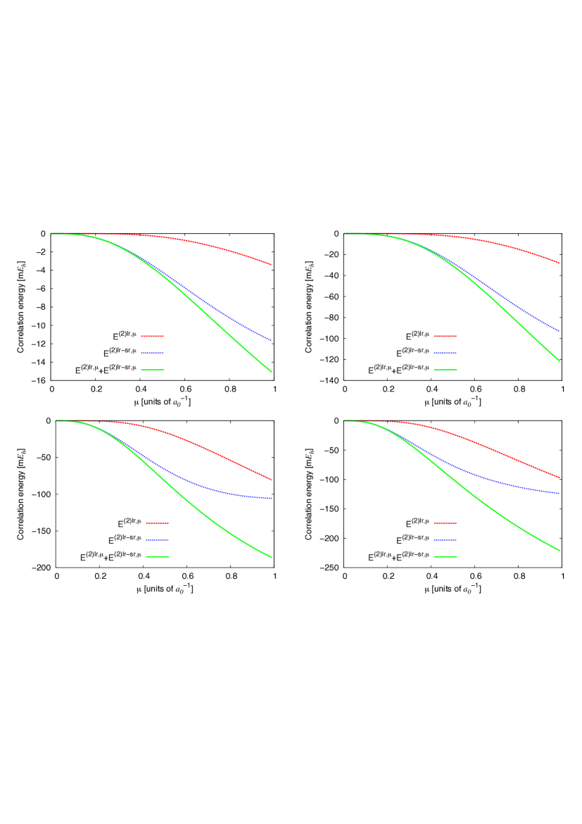
Figure 1: Cornaton et al., Physical Review A

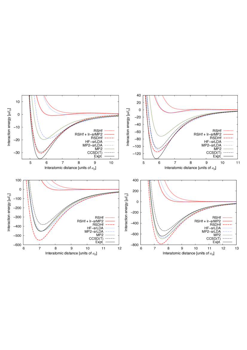
Figure 2: Cornaton et al., Physical Review A

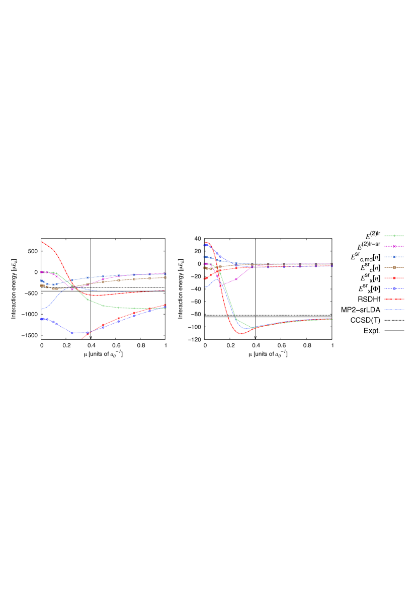
Figure 3: Cornaton et al., Physical Review A

Figure 4: Cornaton et al., Physical Review A

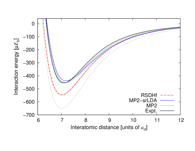
(a)

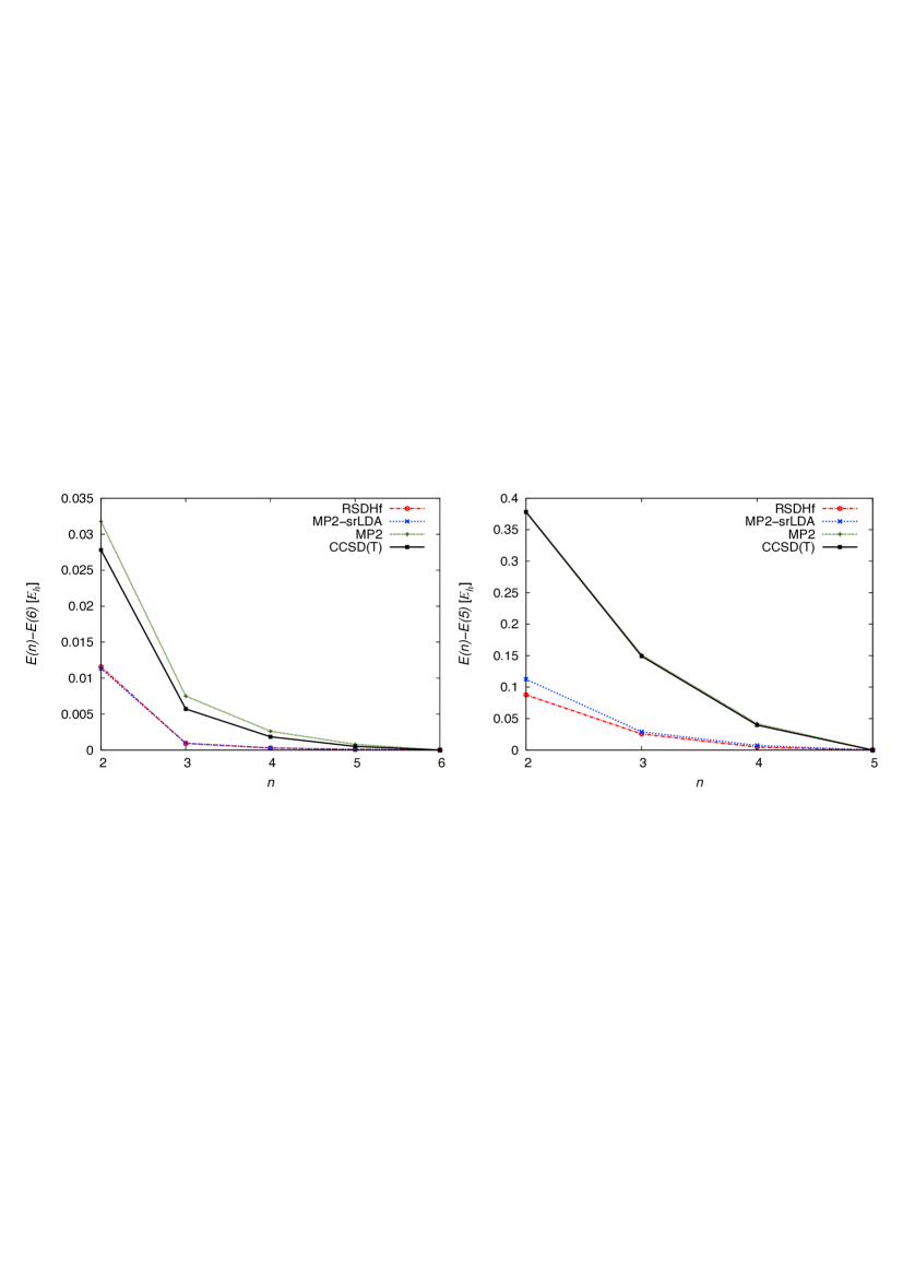
Figure 5: Cornaton et al., Physical Review A

Table 1: Cornaton et al., Physical Review A

		MP2	CCSD(T)	MP2-srLDA	RSDHf	Expt.a
He2	$R_{\rm e}$	5.862 (1.043)	5.690 (1.013)	6.147 (1.094)	5.670 (1.009)	5.618 (1.000)
	$D_{\rm e}$	19.67 (0.564)	29.63 (0.850)	18.81 (0.539)	30.47 (0.874)	34.87 (1.000)
	$\omega_{\rm e}$	24.9 (0.780)	30.3 (0.886)	21.2 (0.620)	31.1 (0.909)	34.2 (1.000)
	$C_{6}$	1.203 (0.815)	1.467 (0.994)	1.613 (1.093)	1.586 (1.075)	1.476 (1.000)
	$\sigma$	5.235 (1.043)	5.066 (1.010)	5.414 (1.079)	5.037 (1.004)	5.018 (1.000)
Ne2	$R_{\rm e}$	6.138 (1.051)	5.952 (1.019)	6.015 (1.030)	5.893 (1.009)	5.839 (1.000)
	$D_{\rm e}$	72.70 (0.542)	105.83 (0.789)	110.87 (0.826)	115.29 (0.859)	134.18 (1.000)
	$\omega_{\rm e}$	20.7 (0.704)	25.7 (0.874)	24.3 (0.827)	22.3 (0.758)	29.4 (1.000)
	$C_{6}$	5.320 (0.821)	7.967 (1.229)	6.819 (1.052)	7.369 (1.137)	6.480 (1.000)
	$\sigma$	5.505 (1.053)	5.331 (1.019)	5.310 (1.015)	5.213 (0.997)	5.230 (1.000)
Ar2	$R_{\rm e}$	7.133 (1.005)	7.227 (1.018)	7.183 (1.012)	7.013 (0.988)	7.099 (1.000)
	$D_{\rm e}$	453.08 (0.997)	382.13 (0.841)	451.32 (0.993)	550.71 (1.212)	454.50 (1.000)
	$\omega_{\rm e}$	30.5 (0.953)	27.9 (0.872)	28.6 (0.893)	33.8 (1.056)	32.0 (1.000)
	$C_{6}$	77.56 (1.174)	66.10 (1.001)	80.43 (1.217)	89.71 (1.358)	66.07 (1.000)
	$\sigma$	6.357 (0.998)	6.454 (1.014)	6.381 (1.002)	6.237 (0.980)	6.367 (1.000)
Kr2	$R_{\rm e}$	7.587 (1.001)	7.729 (1.020)	7.642 (1.008)	7.491 (0.989)	7.578 (1.000)
	$D_{\rm e}$	689.18 (1.078)	541.08 (0.846)	668.02 (1.045)	785.60 (1.229)	639.42 (1.000)
	$\omega_{\rm e}$	24.3 (0.996)	21.6 (0.889)	24.2 (0.996)	26.2 (1.078)	24.3 (1.000)
	$C_{6}$	165.09 (1.230)	129.26 (0.963)	160.30 (1.195)	175.07 (1.305)	134.19 (1.000)
	$\sigma$	6.760 (0.996)	6.906 (1.017)	6.785 (0.999)	6.668 (0.982)	6.789 (1.000)

^a Reference Tang and Toennies (2003)

References

- Ángyán et al. (2005) J. G. Ángyán, I. C. Gerber, A. Savin, and J. Toulouse, Phys. Rev. A, 72, 012510 (2005).
- Fromager and Jensen (2008) E. Fromager and H. J. Aa. Jensen, Phys. Rev. A, 78, 022504 (2008).
- Ángyán (2008) J. G. Ángyán, Phys. Rev. A, 78, 022510 (2008).
- Kullie and Saue (2012) O. Kullie and T. Saue, Chem. Phys., 395, 54 (2012).
- Fromager et al. (2010) E. Fromager, R. Cimiraglia, and H. J. Aa. Jensen, Phys. Rev. A, 81, 024502 (2010).
- Goll et al. (2005) E. Goll, H. J. Werner, and H. Stoll, Phys. Chem. Chem. Phys., 7, 3917 (2005).
- Janesko et al. (2009) B. G. Janesko, T. M. Henderson, and G. E. Scuseria, J. Chem. Phys., 130, 081105 (2009).
- Toulouse et al. (2009) J. Toulouse, I. C. Gerber, G. Jansen, A. Savin, and J. G. Ángyán, Phys. Rev. Lett., 102, 096404 (2009).
- Toulouse et al. (2010) J. Toulouse, W. Zhu, J. G. Ángyán, and A. Savin, Phys. Rev. A, 82, 032502 (2010).
- Toulouse et al. (2004) J. Toulouse, A. Savin, and H. J. Flad, Int. J. Quantum Chem., 100, 1047 (2004a).
- Toulouse et al. (2004) J. Toulouse, F. Colonna, and A. Savin, Phys. Rev. A, 70, 062505 (2004b).
- Gerber and Ángyán (2007) I. C. Gerber and J. G. Ángyán, J. Chem. Phys., 126, 044103 (2007).
- Zhu et al. (2010) W. Zhu, J. Toulouse, A. Savin, and J. G. Ángyán, J. Chem. Phys., 132, 244108 (2010).
- Liu et al. (2011) R. F. Liu, C. A. Franzese, R. Malek, P. S. Zuchowski, J. G. Ángyán, M. S. Szczesniak, and G. Chalasinski, J. Chem. Theory Comput., 7, 2399 (2011).
- Alam and Fromager (2012) M. M. Alam and E. Fromager, Chem. Phys. Lett., 554, 37 (2012).
- Toulouse et al. (2005) J. Toulouse, P. Gori-Giorgi, and A. Savin, Theor. Chem. Acc., 114, 305 (2005).
- Paziani et al. (2006) S. Paziani, S. Moroni, P. Gori-Giorgi, and G. B. Bachelet, Phys. Rev. B, 73, 155111 (2006).
- Helgaker et al. (2004) T. Helgaker, P. Jørgensen, and J. Olsen, “Molecular electronic-structure theory,” (Wiley, Chichester, 2004) pp. 724–816.
- Savin (1996) A. Savin, “Recent developments and applications of modern density functional theory,” (Elsevier, Amsterdam, 1996) p. 327.
- Tang and Toennies (2003) K. T. Tang and J. P. Toennies, J. Chem. Phys., 118, 4976 (2003).
- Pollet et al. (2002) R. Pollet, A. Savin, T. Leininger, and H. Stoll, J. Chem. Phys., 116, 1250 (2002).
- Fromager et al. (2007) E. Fromager, J. Toulouse, and H. J. Aa. Jensen, J. Chem. Phys., 126, 074111 (2007).
- Gerber and Ángyán (2005) I. C. Gerber and J. G. Ángyán, Chem. Phys. Lett., 415, 100 (2005).
- Fromager and Jensen (2011) E. Fromager and H. J. Aa. Jensen, J. Chem. Phys., 135, 034116 (2011).
- Heyd et al. (2003) J. Heyd, G. E. Scuseria, and M. Ernzerhof, J. Chem. Phys., 118, 8207 (2003).
- Heyd and Scuseria (2004) J. Heyd and G. E. Scuseria, J. Chem. Phys., 120, 7274 (2004).
- Gori-Giorgi and Savin (2006) P. Gori-Giorgi and A. Savin, Phys. Rev. A, 73, 032506 (2006).
- Goll et al. (2009) E. Goll, M. Ernst, F. Moegle-Hofacker, and H. Stoll, J. Chem. Phys., 130, 234112 (2009).
- Gori-Giorgi and Savin (2009) P. Gori-Giorgi and A. Savin, Int. J. Quantum Chem., 109, 1950 (2009).
- Hohenberg and Kohn (1964) P. Hohenberg and W. Kohn, Phys. Rev., 136, B864 (1964).
- Sharkas et al. (2011) K. Sharkas, J. Toulouse, and A. Savin, J. Chem. Phys., 134, 064113 (2011).
- Fromager (2011) E. Fromager, J. Chem. Phys., 135, 244106 (2011).
- Ángyán (2009) J. G. Ángyán, J. Math. Chem., 46, 1 (2009).
- Cornaton et al. (2013) Y. Cornaton, O. Franck, A. M. Teale, and E. Fromager, Mol. Phys., 111, 1275 (2013).
- dal (2011) “Dalton2011,” an ab initio electronic structure program. See http://daltonprogram.org/ (2011).
- Dunning Jr. (1989) T. H. Dunning Jr., J. Chem. Phys., 90, 1007 (1989).
- Kendall et al. (1992) R. A. Kendall, T. H. Dunning Jr., and R. J. Harrison, J. Chem. Phys., 96, 6796 (1992).
- Woon and Dunning Jr. (1993) D. E. Woon and T. H. Dunning Jr., J. Chem. Phys., 98, 1358 (1993).
- Woon and Dunning Jr. (1994) D. E. Woon and T. H. Dunning Jr., J. Chem. Phys., 100, 2975 (1994).
- Koput and Peterson (2002) J. Koput and K. A. Peterson, J. Phys. Chem. A, 106, 9595 (2002).
- Wilson et al. (1999) A. K. Wilson, D. E. Woon, K. A. Peterson, and T. H. Dunning Jr., J. Chem. Phys., 110, 7667 (1999).
- Marquardt (2012) R. Marquardt, J. Math. Chem., 50, 577 (2012).
- Fromager et al. (2009) E. Fromager, F. Réal, P. Wåhlin, U. Wahlgren, and H. J. Aa. Jensen, J. Chem. Phys., 131, 054107 (2009).
- Strømsheim et al. (2011) M. D. Strømsheim, N. Kumar, S. Coriani, E. Sagvolden, A. M. Teale, and T. Helgaker, J. Chem. Phys., 135, 194109 (2011).
- Toulouse et al. (2011) J. Toulouse, W. Zhu, A. Savin, G. Jansen, and J. G. Ángyán, J. Chem. Phys., 135, 084119 (2011).