Polar optical phonons in core-shell semiconductor nanowires

Abstract

We obtain the the long-wavelength polar optical vibrational modes of semiconductor core-shell nanowires by means of a phenomenological continuum model. A basis for the space of solutions is derived, and by applying the appropriate boundary conditions, the transcendental equations for the coupled and uncoupled modes are attained. Our results are applied to the study of the GaAs-GaP core-shell nanowire, for which we calculate numerically the polar optical modes, analyzing the role of strain in the vibrational properties of this nanosystem.

I Introduction

The study of semiconductor nanowires is of the utmost importance for the progress of the design and fabrication of novel devices and the investigation of fundamental phenomena. The development of growth techniques has allowed for the fabrication of high quality systems. Among these, the core-shell architecture is of great interest:Peidong a cylindrical core of a semiconductor material is surrounded by a shell of a different semiconductor, usually with a larger bandgap. In this way, it provides a means of removing surface states and separating the carriers, or as a waveguide or cavity for optoelectronic applications. Furthermore, if the core and shell materials are grown with a lattice mismatch, the strain can be employed as an additional degree of freedom for band structure engineering. These particular systems have been synthesized employing different pairs of core-shell materials, such as GaAs-GaAsP,Hua2009 InAs-GaAs,Niquet2007 GaN-GaP,Hung-Min2003 GaP-GaN,Hung-Min2003 GaAs-GaP,Montazeri2010 AlN-GaN,Zhang GaAsP-GaP,Mohseni , GaAs-AlGaAs,Bailon and CdSe/CdS,Giugni2012 among others. A great variety of applications for these core-shell nanowires have appeared, for instance, nanowire lasers,Hua2009 nanowire nanosensors,Cui ; Zheng photovoltaic devicesDong and light emission diodes,Minot to name a few.

Polar optical phonons are of a great interest for the spectroscopic characterization of core-shell nanowires of compound semiconductors. Raman scattering provides information on the phonon frequencies, which can be related to the strain in the core and the shell of the nanowires. However, in spite of its importance for their spectroscopic characterization, up to our knowledge, only a few calculations of interface modes in GaN/AlN core-shell nanowires have been reported recently, mainly obtained by means of a macroscopic dielectric model. cross

In this work we address this issue, employing a phenomenological continuum model for polar optical phonons in the long-wave limit in a cylindrical core-shell geometry. Indeed, polar optical oscillations have been successfully studied for different nanostructures applying a long-wavelength approximation and based on different continuum approaches; see, for example, Refs. CubaLibro, ; StroscioDutta2001, ; ridley, and references therein. In particular, oscillations in cylindrical systems have been studied in Refs. Stroscio, ; Enderlein, ; Comas1995, , but only for solid nanowires made of a single material, and in some cases neglecting the dispersion along the nanowire axis.

In order to study polar phonons in core-shell nanowires, we follow the approach employed for other geometries, as outlined in Refs. CubaLibro, ; Comas1995, , and originally exposed in Ref. CTG92, . This phenomenological continuum model (PCM) takes into account the coupled electro-mechanical character of the vibrations without making any simplifying assumptions. From the prior experience in quasi-two-dimensional CubaLibro and quasi-zero-dimensional systems,Roca1994 as it was shown in Refs. CTG92, ; CTG94, ; Comas94, , we do know that no further hypotheses as to the electromechanical coupling should be made when searching for linearly independent solutions in these quasi-one-dimensional structures. Some previous work following this approach has been made for cylindrical geometries,Comas1995 albeit for simple (i.e., solid and with only one material) nanowires and without considering the dependence on the axial coordinate. Here we generalize this work, considering all types of polar oscillation modes in core-shell nanowires. To this end we focus in obtaining a basis function with cylindrical symmetry, taking into account the possible angular and axial dependence the modes may have. We apply the appropriate boundary conditions for core-shell modes to a general solution, given by a linear combination of the basis functions. As we concentrate in materials with very different bulk values of their mechanical parameters, we can impose a total confinement of the mechanical components. This condition leads to the mixing of the different modes. Indeed, phonon modes of mixed nature are obtained and may display predominant longitudinal optical ($LO$), transverse optical ($TO$) or interface ($I$) profiles in the different regions of the vibrational spectra. We analyze the character of the phonon modes, and give detailed numerical results for one particular case, namely, the GaAs-GaP core-shell nanowire.

The paper is organized as follows: In Sec. II we present the fundamental equations which describe the polar oscillation modes, discussing their physical meaning and obtaining a basis for the cylindrical geometry. Sec. III explains the obtention of the polar optical modes in core-shell nanowires by applying the appropriate boundary conditions. The solution for the interface optical modes for the core-shell nanowires with cylindrical cross section in the framework of the dielectric continuum model is presented in Sec. IV. Sec. V discusses the inclusion of strain effects in our model. In Sec. VI the results corresponding to a particular example, the GaAs-GaP core-shell nanowire, are presented. In Sec. VII we draw our conclusions.

II The phenomenological continuum model in cylindrical coordinates

We briefly recall here the formalism of the PCM employed in this work. Following the procedure developed in Refs. CTG92, ; CTG94, ; Comas94, , the fundamental equations of motion which include the bulk phonon dispersion are given by

$$\rho_{m}(\omega^{2}-\omega_{TO}^{2})\vec{u}=\rho_{m}\beta_{L}^{2}\nabla(\nabla\cdot\vec{u})-\rho_{m}\beta_{T}^{2}\nabla\times\nabla\times\vec{u}+\alpha\nabla\varphi,$$ (1)

and

$$\nabla^{2}\varphi=\frac{4\pi\alpha}{\varepsilon_{\infty}}\nabla\cdot\vec{u},$$ (2)

with the parameter $\alpha$ defined as

$$\alpha^{2}=\frac{(\varepsilon_{0}-\varepsilon_{\infty})\rho_{m}\omega^{2}_{TO}}{4\pi}.$$ (3)

In these expressions, $\omega_{TO}$ is the transversal bulk frequency at the $\Gamma$ point, $\rho_{m}$ is the reduced mass density, $\beta_{L}$ ($\beta_{T}$) describes the quadratic dispersion of the $LO$ ($TO$)-bulk phonon dispersion of the optical modes in the long-wave limit, and $\varepsilon_{0}$ ($\varepsilon_{\infty}$) is the static (high frequency) dielectric constant. The relative mechanical displacement of the ions is represented by $\vec{u}$ and the electric potential due to the polar character of the vibrations is denoted by $\varphi$. In this model the equations are treated in the quasi-stationary approximation so a harmonic time dependence is considered for all the involved quantities.

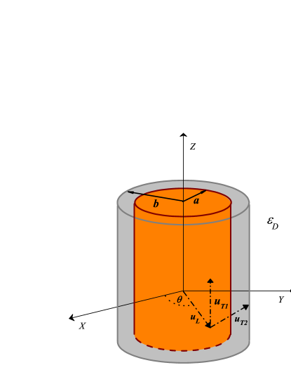
Figure 1: (Color online) Schematic representation of the capped wire system under study. In our case, the material in the core is GaAs and GaP in the shell. $a$ ($b$) is the core (shell) radius. Vibrational phonon amplitudes $u_{L}$, $u_{T1}$, and $u_{T2}$ are indicated. The effect associated to the embedding matrix on the vibrational modes is characterized by an outer dielectric constant $\varepsilon_{D}$.

Eqs. (1) and (2) represent a system of four coupled partial differential equations which describe the confined polar optical phonons in each region of the semiconductor heterostructure. In this particular case, hybrid core-shell cylindrical nanowires consist of a material “$s$” grown on a core structure of material “$c$” , and the medium properties are considered piecewise, as depicted in Fig. 1. Furthermore, the nanowire is embedded in a host material, which is typically a silicate matrix or an organic polymeric compound.

We model the core-shell nanowire as an infinite cylinder of circular cross section with radius $a$, dressed by a cylindrical shell of another material with external radius $b$ (see figure 1). The wire is embedded in a host material uncoupled to the oscillations of the nanowire, characterized by its dielectric constant $\varepsilon_{D}$.

In order to find a general solution for the oscillations of the nanowire, we have to find a basis for the solutions in each region. With this purpose, we follow the method of the potentials described in detail in the book by Morse and Feshbach,Morse that we sketch briefly.

First, we introduce the auxiliary potentials $\vec{\Gamma}$ and $\Lambda$ such that

$$\vec{\Gamma}=\nabla\times\vec{u}\;\;\;\text{and}\;\;\;\Lambda=\nabla\cdot\vec{u}\;.$$ (4)

Taking the curl and the divergence of Eq. (1), we obtain the following new equations for the potentials:

$$\nabla^{2}\vec{\Gamma}+Q_{T}^{2}\vec{\Gamma} = \vec{0},$$ (5)

$$\nabla^{2}\Lambda+Q_{L}^{2}\Lambda = 0,$$ (6)

with $Q_{T},Q_{L}$ given by

$$Q^{2}_{T}=\frac{\omega^{2}_{TO}-\omega^{2}}{\beta^{2}_{T}},$$ (7)

$$Q^{2}_{L}=\frac{\omega^{2}_{LO}-\omega^{2}}{\beta^{2}_{L}}.$$

It can be seen that the solution of Eq. (2) can be written as

$$\varphi=\varphi_{H}-\frac{4\pi\alpha}{\varepsilon_{\infty}Q^{2}_{L}}\Lambda,$$

where $\varphi_{H}$ is the solution of the Laplace equation $\nabla^{2}\varphi_{H}=0$. Moreover, straightforward mathematical manipulations lead us to the following expression for $\vec{u}$:

$$\vec{u}=-\nabla\left[\frac{\alpha}{\rho_{m}\beta^{2}_{T}Q^{2}_{T}}\varphi_{H}+\frac{\Lambda}{Q^{2}_{L}}\right]+\frac{1}{Q^{2}_{T}}\nabla\times\vec{\Gamma}.$$ (8)

In order to obtain the general solution for the relative mechanical displacement $\vec{u}$ and the electric potential $\varphi_{H}$ it is necessary to solve the Helmholtz equations for $\Lambda$ and $\vec{\Gamma}$ and the Laplace equation for $\varphi_{H}$. The solutions for $\Lambda$ and $\varphi_{H}$ are obtained in the standard way; the method for solving the Helmholtz vectorial equation (5) in cylindrical coordinates is reported in Refs. Ruppin, ; Morse, . Nevertheless, in the general case of cylindrical symmetry the displacement vector (8) cannot be decoupled into two independent directions with pure longitudinal ($L$) or transversal motion ($T$). As we state below, only under particular conditions we are able to decouple the motion in $L$ and $T$ independent oscillations. It is convenient to express the vector potential $\vec{\Gamma}$ as a linear combination of the vectors $\vec{M}$ and $\vec{N}$,

$$\vec{M} = \nabla\times(\upsilon_{1}\vec{\kappa}),$$ (9)

$$\vec{N} = \frac{1}{Q^{2}_{T}}\nabla\times\nabla\times(\upsilon_{2}\vec{\kappa}),$$

where $\upsilon_{i},(i=1,2)$ are linearly independent solutions of the scalar equation $\nabla^{2}\upsilon_{i}+Q^{2}_{T}\upsilon_{i}=0$ and, in cylindrical geometry, $\vec{\kappa}=\vec{e}_{z}$.

Once the functions $\Lambda$, $\vec{\Gamma}$ and $\varphi_{H}$ have been obtained, it is easy to prove that the general solution of Eqs. (1) can be expressed in terms of the analytical basis functions for the space of solutions, given by

$$F_{T1} = \left(\begin{array}[]{c}\vec{u}_{T1}\\ \varphi_{T1}\\ \end{array}\right)=\left(\begin{array}[]{c}\frac{ik_{z}}{q_{T}}f_{n}^{\prime}(q_{T}\rho)\\ -\frac{nk_{z}}{q_{T}}\frac{1}{q_{T}\rho}f_{n}(q_{T}\rho)\\ f_{n}(q_{T}\rho)\\ 0\\ \end{array}\right)e^{i(n\theta+k_{z}z)}$$ (16)

$$F_{T2} = \left(\begin{array}[]{c}\vec{u}_{T2}\\ \varphi_{T2}\\ \end{array}\right)=\left(\begin{array}[]{c}\frac{in}{q_{T}\rho}f_{n}(q_{T}\rho)\\ -f^{\prime}_{n}(q_{T}\rho)\\ 0\\ 0\\ \end{array}\right)e^{i(n\theta+k_{z}z)}$$ (23)

$$F_{L} = \left(\begin{array}[]{c}\vec{u}_{L}\\ \varphi_{L}\\ \end{array}\right)=\left(\begin{array}[]{c}f^{\prime}_{n}(q_{L}\rho)\\ \frac{in}{q_{L}\rho}f_{n}(q_{L}\rho)\\ \frac{ik_{z}}{q_{L}}f_{n}(q_{L}\rho)\\ \frac{4\pi\alpha}{\varepsilon_{\infty}}\frac{1}{q_{L}}f_{n}(q_{L}\rho)\end{array}\right)e^{i(n\theta+k_{z}z)}$$ (30)

$$F_{H} = \left(\begin{array}[]{c}\vec{u}_{H}\\ \varphi_{H}\\ \end{array}\right)=\left(\begin{array}[]{c}g^{\prime}_{n}(k_{z}\rho)\\ \frac{in}{k_{z}\rho}g_{n}(k_{z}\rho)\\ g_{n}(k_{z}\rho)\\ -\frac{\rho_{m}\beta^{2}_{T}q^{2}_{T}}{\alpha}\frac{1}{k_{z}}g_{n}(k_{z}\rho)\end{array}\right)e^{i(n\theta+k_{z}z)},$$ (37)

where the matrix components are understood in the form $(u_{\rho},u_{\theta},u_{z},\varphi)$; the prime denotes the derivative with respect to the argument; $n$ is an integer label related to the angular dependence of the modes; and $k_{z}$ is the continuum wavevector along the cylinder axis. Additionally, we introduce the wavenumbers

$$q^{2}_{L,T} = Q^{2}_{L,T}-k_{z}^{2}\;.$$ (38)

If $q^{2}_{L,T}>0$ ($q^{2}_{L,T}<0$) the function $f_{n}$ is an order-$n$ Bessel (modified Bessel) function of the first or second kind, i.e., Bessel $J_{n}$ or Neumann $N_{n}$ (Infeld $I_{n}$ or MacDonald $K_{n}$). On the other hand, $g_{n}$ is an order-$n$ modified Bessel function of the first or second kind, i.e., Infeld $I_{n}$ or MacDonald $K_{n}$. We follow the definitions and conventions of Abramowitz and Stegun. AbramowitzStegun1964 It is important and straightforward to check that $\nabla\times\vec{u}_{L}=\nabla\times\vec{u}_{H}=\vec{0}$ and $\nabla\cdot\vec{u}_{T1}=\nabla\cdot\vec{u}_{T2}=\nabla\cdot\vec{u}_{H}=0$.

Particular cases of this basis have been used to study phonon modes in non-polar nanotubes ChicoRPA2004 ; CPC2006 and in solid nanowires with only one material at $k_{z}=0$. Comas1993a

III Polar optical oscillation modes in core-shell nanowires

In order to obtain the particular solution for the core-shell geometry, boundary conditions for $\vec{u}$ and $\varphi$ at each interface should be applied. With respect to the electromagnetic magnitudes, we have that the electric potential $\varphi$ and the normal component of the displacement field $\vec{D}$ should be continuous at the interfaces. Recall that the electric displacement vector is given byCubaLibro $\vec{D}=4\pi\alpha\vec{u}-\varepsilon_{\infty}\nabla\cdot\varphi$. However, we will consider pairs of core-shell materials with disparate mechanical properties, so the oscillations occurring in one of them do not penetrate significantly into the other. This is the case of the GaAs-GaP core-shell nanowire discussed in this work; in fact, a significant number of pairs of materials of current interest satisfies this requisite. With this assumption, it can be adopted an approximate boundary condition of complete mechanical confinement, $\vec{u}|_{S}=0$. Thus, the matching boundary conditions are reduced to

$$\left.\vec{u}\right|_{S} = 0,$$

$$\left.\varphi^{-}\right|_{S} = \left.\varphi^{+}\right|_{S},$$ (39)

$$\left.\varepsilon^{-}_{\infty}\frac{\partial\varphi^{-}}{\partial\rho}\right|_{S} = \left.\varepsilon^{+}_{\infty}\frac{\partial\varphi^{+}}{\partial\rho}\right|_{S}.$$

In Eqs. (III) the symbol $-$(+) represents that the associated quantity is evaluated at the inside (outside) of the corresponding interfaces, namely, the cylindrical surfaces of radius $a$ and $b$. The dispersion relations are then obtained applying these boundary conditions (III) to a general linear combination of the basis functions, that can be written as

$$F=\left\{\begin{array}[]{cc}\sum\limits_{M}A_{M}^{(c)}F_{M}^{(1)};&\rho\leq a\\ \sum\limits_{M}A_{M}^{(s)}F_{M}^{(1)}+\sum\limits_{M}B_{M}^{(s)}F_{M}^{(2)};&a\leq\rho\leq b\\ \sum\limits_{M}B_{M}^{(D)}F_{M}^{(2)};&\rho\geq b\end{array}\right.$$ (43)

where $M=T1,T2,L,H$ and $i=1,2$ denotes that the corresponding Bessel and modified Bessel functions $f_{n}$, $g_{n}$ appearing the basis functions $F_{M}^{(i)}$ are or the first or the second kind respectively.

IV Interface optical phonons

The system of Eqs. (1) and (2) lead to coupled modes at the interfaces. These modes shows a predominant electric character associated to the system interfaces and are related to interface phonons (IP). For a simple characterization and for sake of comparison with the present theoretical model, we calculate the IP employing the dielectric continuum approach (DCA). Considering that the electric field satisfies quasistatic Maxwell equations, we have

$$\varepsilon_{c(s)}(\omega)\nabla^{2}\varphi=0,$$

where the frequency dependent dielectric function $\varepsilon_{c(s)}(\omega)$ for the core (shell) is given by the standard expression

$$\varepsilon_{c(s)}(\omega)=\varepsilon_{\infty}^{c(s)}\frac{\omega_{LO}^{c(s)2}-\omega^{2}}{\omega_{TO}^{c(s)2}-\omega^{2}}.$$ (44)

In the above equation $\omega_{LO}^{c(s)}$ and $\omega_{TO}^{c(s)}$ are the bulk longitudinal and transversal polar optical phonons frequencies at the $\Gamma$ point for the core (shell) semiconductor material. The IP satisfy the Laplace equation $\nabla^{2}\varphi=0$ and $\varepsilon_{c(s)}(\omega)\neq 0.$ Thus, employing the standard electrostatic boundary condition at the interfaces we obtain

$$(\varepsilon_{c}(\omega)-\varepsilon_{s}(\omega))(\varepsilon_{D}-\varepsilon_{s}(\omega))I_{n}(k_{z}a)I_{n}^{\prime}(k_{z}a)K_{n}(\gamma k_{z}a)K_{n}^{\prime}(\gamma k_{z}a) -$$

$$(\varepsilon_{c}(\omega)K_{n}(k_{z}a)I_{n}^{\prime}(k_{z}a)-\varepsilon_{s}(\omega)I_{n}(k_{z}a)K_{n}^{\prime}(k_{z}a)) \times$$

$$(\varepsilon_{d}I_{n}(\gamma k_{z}a)K_{n}^{\prime}(\gamma k_{z}a)-\varepsilon_{s}(\omega)K_{n}(\gamma k_{z}a)I_{n}^{\prime}(\gamma k_{z}a)) = 0,$$ (45)

where $\gamma=b/a$ is the ratio between the shell and core radii. Equation (45) gives the dispersion relations of IP as a function of $k_{z}$ and the parameter $\gamma$ for different values of $n=0,1,2,..$. In the case of $k_{z}=0$ Eq. (45) is reduced to

$$(\varepsilon_{c}(\omega)-\varepsilon_{s}(\omega))(\varepsilon_{D}-\varepsilon_{s}(\omega))-(\varepsilon_{c}(\omega)+\varepsilon_{s}(\omega))(\varepsilon_{D}+\varepsilon_{s}(\omega))\gamma^{2n}=0.$$

Equation (45) shows that for each value of $n$ we have three independent IP branches. One is linked to the cylindrical core embedded in a host material with an effective dielectric constant, and the other two correspond to the cylindrical shell structure sandwiched between the core and a host dielectric medium. These interface phonons depend on the geometrical parameter $\gamma$.

V Strain effects

It is important to note that in semiconductor core-shell nanowires, strain effects cannot be neglected. To model these, we applied the same procedure as in Ref. paperanterior, , and we study its importance by comparing to the strain-free case.

The shift in the optical phonon frequencies due to the strain in the core-shell nanowire is given bySpanier ; Dohcevic

$$\Delta\omega_{i}=-\gamma_{i}\omega_{i}\frac{\Delta V}{V},$$ (46)

where $i=LO,TO$, $\gamma_{i}$ is the Grüneisen parameter, $V$ is the volume of unit cell, and $\Delta V$ is the volume change due to the lattice mismatch. The relation $\frac{\Delta V}{V}=\mathrm{tr}(\varepsilon)$, where $\mathrm{tr}(\varepsilon)$ is the trace of the stress tensor, can be evaluated for the core and shell materials in cylindrical geometry,Menendez yielding

$${\rm tr}(\varepsilon_{c}) = -2\varepsilon_{\rm misfit}\left(\frac{(1+\nu_{c})(1-2\nu_{c})(\gamma^{2}-1)}{(1-E_{r})(1-2\nu_{c})-(1-2\nu_{c}+E_{r})\gamma^{2}}+\frac{\nu_{c}(\gamma^{2}-1)}{(\gamma^{2}-1)+E_{r}}\right)+\varepsilon_{\rm misfit}\left(\frac{(\gamma^{2}-1)}{(\gamma^{2}-1)+E_{r}}\right),$$ (47)

$${\rm tr}(\varepsilon_{s}) = 2\varepsilon_{\rm misfit}\left(\frac{(1+\nu_{s})(1-2\nu_{s})E_{r}}{(1-E_{r})(1-2\nu_{s})-(1-2\nu_{s}+E_{r})\gamma^{2}}+\frac{\nu_{s}E_{r}}{(\gamma^{2}-1)+E_{r}}\right)-\varepsilon_{\rm misfit}\frac{E_{r}}{(\gamma^{2}-1)+E_{r}},$$ (48)

with $\nu_{c}$, $\nu_{s}$ the Poisson ratios of the core and shell materials respectively; the lattice mismatch is $\varepsilon_{\mathrm{misfit}}=(a_{s}-a_{c})/a_{c}$ with $a_{c}$ $(a_{s})$ being the cubic lattice constant of the core (shell) material; $E_{r}=E_{c}/E_{s}$ is the ratio between the core and shell Young moduli. From Eqs. (47) and (48) we obtain the following limits

$$\mathrm{tr}(\varepsilon_{c})_{\lim\gamma\rightarrow 1} = 0;$$ (49)

$$\ \ \mathrm{tr}(\varepsilon_{s})_{\lim\gamma\rightarrow 1} = 2\varepsilon_{\mathrm{misfit}}\frac{1-2\nu_{c}}{\nu_{c}-1};$$

$$\mathrm{tr}(\varepsilon_{c})_{\lim\gamma\rightarrow\infty} = \varepsilon_{\mathrm{misfit}}\frac{(1-2\nu_{c})\left(3+\nu_{c}\right)}{1-2\nu_{c}+E_{r}};$$ (50)

$$\mathrm{tr}(\varepsilon_{s})_{\lim\gamma\rightarrow\infty} = 0.$$

These equations allow us to include strain effects on the phonon frequencies in our model, replacing in Eqs. (7) and (45) the unstrained bulk frequencies at $\Gamma$, $\omega_{TO}$ and $\omega_{LO}$, by $\omega_{T}(\gamma)$, $\omega_{L}(\gamma)$:

$$\omega_{T}(\gamma) = \omega_{TO}+\Delta\omega_{TO}(\gamma);$$ (51)

$$\omega_{L}(\gamma) = \omega_{LO}+\Delta\omega_{LO}(\gamma).$$ (52)

VI Results

In what follows we present some analytical and numerical results for core and shell modes, without and with stress effects. As commented above, we choose as a representative example the GaAs/GaP core-shell nanowire. The parameters chosen for these two materials are listed in Table 1. Since the $k_{z}=0$, $n=0$ case has been analyzed elsewhere, paperanterior we focus on $k_{z}=0$, $n>0$ and $k_{z}\neq 0$, $n=0,1$ cases. In order to avoid a heavy notation, we drop the indices $c$, $s$ in the parabolicity parameters and in the bulk frequencies when there is no possible ambiguity.

Table 1: Bulk parameters for GaAs and GaP in zinc blende phase.

Material	$\epsilon_{0}$	$\epsilon_{\infty}^{*}$	$\omega_{TO}$ (cm-1)	$\omega_{LO}$ (cm-1)	$\beta_{T}(\times 10^{-6})$	$\beta_{L}(\times 10^{-6})$	$\gamma_{TO}$	$\gamma_{LO}$	$E$ (1012 dyn/cm2)	$\nu$	$a_{0}$ (nm)
GaAs	12.80a	11.26	267a	285a	1.70b	1.76b	1.11d	0.97d	0.853d	0.312d	0.565d
GaP	11.11a	9.15	365.3a	402.5a	0.72c	1.60c	1.09d	0.95d	1.03d	0.306d	0.545d

a) Ref. Martienssen, ; b) Ref. CubaLibro, ; c) Ref. Borcherds, ; d) Ref. Adachi, .
^∗Using the Lyddane-Sachs-Teller relation.

VI.1 Modes with $n\neq 0$, $k_{z}=0$

VI.1.1 Core modes

Assuming complete mechanical confinement, we model core modes by considering $\vec{u}\equiv 0$ for $a<\rho<b$ and $\vec{u}\neq 0$ for $\rho<a$. The application of the boundary conditions indicated in Eqs. (III) yields one family of uncoupled $T1$ modes and one of coupled $L$-$T2$ modes. This decoupling of the $T1$ modes is evident from the expressions of the basis functions (16) for $k_{z}=0$. The eigenvalue equations for the uncoupled $T1$ modes are given by $J_{n}(\mu^{(m)}_{n})=0,m=1,2,...$ which yield the dispersion relations $\omega^{2}=\omega_{TO}^{2}-(\mu^{(m)}_{n}\beta_{T}/a)^{2}$.

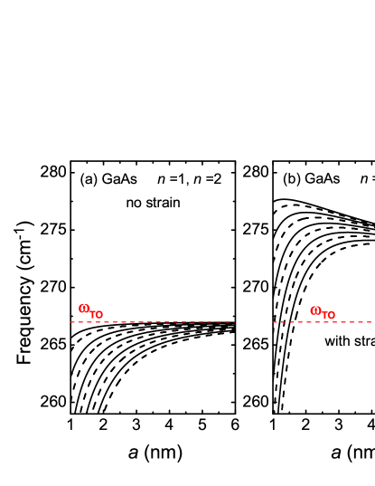
Figure 2: (Color online) GaAs optical uncoupled transversal phonon modes at $k_{z}=0$ for $n=1$ (full lines) and $n=2$ (dashed lines) in a GaAs-GaP core-shell nanowire as a function of the core radius $a$. Panel (a) without strain; panel (b)including strain effects. For the calculation represented in panel (b) we fixed $b-a=3$ nm. The bulk GaAs TO phonon frequency is indicated by a red (gray) horizontal dashed line.

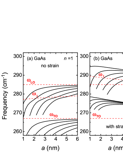
Figure 3: (Color online) GaAs optical coupled phonon modes at $k_{z}=0$ for $n=1$ in GaAs-GaP core-shell nanowire as a function of the core radius $a$. Panel (a) neglecting strain effects, panel (b) including strain. In the calculation we fixed the value of $b-a=3$ nm and $\varepsilon_{D}=2.56$. The bulk GaAs $LO$ and $TO$ phonon frequencies are indicated by gray (red) dashed lines. The corresponding interface phonon frequency obtained in the framework of the DCA is also represented by a gray (red) dashed line.

Figure 2 shows the frequency dependence of the confined modes on the core radius $a$ for the GaAs-GaP core-shell nanowire. For the strain-free case (Fig. 2 (a)), the mode frequency is independent of the shell radius $b$, so it is similar to an undressed quantum wire. This behavior changes when the effects of strain are taken into account, which yields the eigenfrequencies dependent on the shell radius $b$. As in the $n=0$ case, there is an increase on the frequencies of the modes when considering strain effects, clearly shown in Fig. 2 (b). Following the results of the Appendix for the coupled $L$-$T2$ core modes, the secular equation (76) is reduced to the following:

$$\left[J^{\prime}_{n}(t_{c})-\frac{n}{t_{c}}J_{n}(t_{c})\right]\left[J^{\prime}_{n}(l_{c})-C_{1}\frac{n}{l_{c}}J_{n}(l_{c})\right]-C_{2}\left[1-\frac{\omega^{2}}{\omega_{TO}^{2}}\right]\left[J^{\prime}_{n}(t_{c})J^{\prime}_{n}(l_{c})-\frac{n^{2}}{t_{c}l_{c}}J_{n}(t_{c})J_{n}(l_{c})\right]=0,$$ (53)

where

$$C_{1} = \frac{\varepsilon^{s}_{\infty}[(\varepsilon_{D}-\varepsilon^{s}_{\infty})+\gamma^{2n}(\varepsilon_{D}+\varepsilon^{s}_{\infty})]}{\varepsilon^{c}_{\infty}[(\varepsilon_{D}-\varepsilon^{s}_{\infty})-\gamma^{2n}(\varepsilon_{D}+\varepsilon^{s}_{\infty})]},$$ (54)

$$C_{2} = \frac{[(\varepsilon^{s}_{\infty}-\varepsilon^{c}_{\infty})(\varepsilon_{D}-\varepsilon^{s}_{\infty})+\gamma^{2n}(\varepsilon^{c}_{\infty}+\varepsilon^{s}_{\infty})(\varepsilon_{D}+\varepsilon^{s}_{\infty})]}{(\varepsilon^{c}_{0}-\varepsilon^{c}_{\infty})[(\varepsilon_{D}-\varepsilon^{s}_{\infty})-\gamma^{2n}(\varepsilon_{D}+\varepsilon^{s}_{\infty})]},\;$$

and $t_{c}=q_{T}a$, $l_{c}=q_{L}a$. Sub- or superindices $c$, $s$, indicate that the corresponding quantities (i.e., $q_{T,L}$ or the dielectric constants $\varepsilon_{0}$, $\varepsilon_{\infty}$) correspond to the core or shell materials respectively.

The phonon frequencies for $n=1$ as a function of core radius $a$, given by Eq. (53), are presented in Fig. 3. The interface ($I$) mode manifests in the abrupt change of slope in the frequencies, where the mixing between longitudinal and transversal modes occurs. The electrostatic potential of the surface oscillation is manifested when the interaction of the $LO$-confined phonon with the surface mode becomes strong for certain values of the core radius $a$. In this region the electric character of the modes is dominant. As $a\rightarrow\infty$, the bulk $LO$ and $TO$ phonon dispersion relations are recovered. The effect of strain is also an increase of the phonon frequencies (Fig. 3 (b)). Notice the characteristic change of the slope in Figs. 2 (b) and 3 (b) when the strain is considered. As the core radius increases, the parameter $\gamma\rightarrow 1$ and the phonon frequencies decrease, reaching the bulk limit $\omega_{T(L)}(\gamma=1)=\omega_{TO(LO)}$; then, the spatial confinement and the influence of the strain (see Eq. (49)) on the core are negligible.

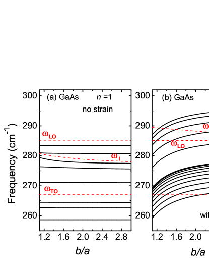
Figure 4: (Color online) The same asFig. (3) as a function of the ratio $b/a$, fixing the value of $a=3$ nm and$\varepsilon_{D}=2.56$. The corresponding interface optical phonon ($I$-phonon) frequency obtained from Eq. (45) is also represented by a gray (red) dashed line.

Figure 4 shows the coupled core modes at $k_{z}=0$ for $n=1$ as a function of the ratio $b/a$. As it can be seen, the core modes depend very weakly on the ratio $b/a$ if strain effects are neglected (Fig. 4 (a)). Only the third mode in order of decreasing frequency shows a certain dependence on $\gamma$. This is due to the mixture between longitudinal and transversal modes near the interface phonon frequency $\omega_{I}$ produced by the strong interaction of the electrostatic potential with the interface phonon (see Fig. 4(a)). When strain effects are taken into account the $\gamma$ dependence is governed mainly by them, producing an upward shift of the mode frequencies Fig. 4(b). When the shell thickness is much larger than the core radius, $\gamma\gg 1$, the phonon modes feel a residual stress described by Eq. (V), so the frequencies of the transversal ($\omega_{T}(\gamma\rightarrow\infty)$) and longitudinal modes ($\omega_{L}(\gamma\rightarrow\infty)$) reach the limit value 279.54 cm^-1 and 296.70 cm^-1 respectively.

VI.1.2 Shell modes

Complete mechanical confinement in the shell amounts to $\vec{u}\equiv 0$ for $\rho<a$ but $\vec{u}\neq 0$ for $a<\rho<b$. As in the core case, the basis functions (16) when $k_{z}=0$ show that the mode $T1$ is decoupled from the rest, while there is $L$-$T2$ coupling. Indeed, the matching boundary conditions (III) lead to one family of uncoupled $T1$ modes and one of coupled $L$-$T2$ modes, that we describe in the following.

The secular equation for the uncoupled $T1$ shell modes takes the form

$$J_{n}(\mu_{n}^{(m)})N_{n}(\gamma\mu_{n}^{(m)})-J_{n}(\gamma\mu_{n}^{(m)})N_{n}(\mu_{n}^{(m)})=0,$$ (55)

with the dispersion relation $\omega^{2}(\gamma)=\omega_{TO}^{2}-(\mu_{n}^{(m)}\beta_{T}/a)^{2}$, where the frequencies and parabolicity parameters correspond to the shell case An essential difference is observed with respect to core case, namely, that the mode frequency depends on both core and shell radius. This dependence is shown in Fig. 5 for the modes $n=1,2$. It is possible to show that the eigenvalues $\mu_{n}^{(m)}\rightarrow 0$ as $\gamma\rightarrow\infty$, and because the shift $\Delta\omega_{TO}(\gamma\rightarrow\infty)\rightarrow 0$ (see Eq. (V)), the confined modes tend to the corresponding bulk $TO$ phonon frequency, i.e., that of GaP.

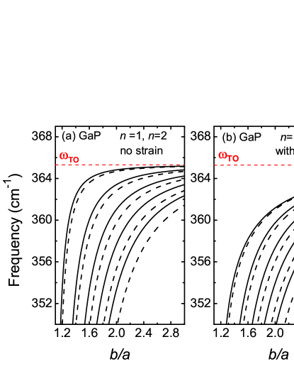
Figure 5: (Color online) GaP optical uncoupled ($T1$) phonon $n=1$ and $n=2$ shell modes at $k_{z}=0$, for a GaAs-GaP core-shell nanowire with fixed $a=3$ nm, as a function of the ratio $\gamma=b/a$. Panel (a) shows the results without strain effects, and panel (b) including strain. The bulk $TO$ phonon frequency for GaP is indicated by a gray (red) dashed line.

The boundary conditions (III) for the shell modes yields a set of equations for the coupled $L$-$T2$ modes, which we give in detail in the Appendix. From Eqs. (76) we obtain the phonon dispersion relation (unstrained and strained cases) with $\gamma=b/a$ for $n=1$ and $k_{z}=0$, shown in Fig. 6. Notice the two interface shell branches $I1$ and $I2$ (shown by gray(red) dashed lines), solutions of Eq. (IF). For frequencies near the interface phonons $\omega_{I1}$ and $\omega_{I2}$, there is a remarkable mixing between the longitudinal and transversal modes. This effect is more remarkable for phonon frequencies $\omega$ near $\omega_{I2}$, where the anticrossing between two modes with different symmetry is stronger if compared with the upper interface branch $I1$. Fig. 6 shows that the interface strain pushes down the phonon shell modes with respect to the bulk phonon frequencies. Recall that in the core the effect is the opposite (see Fig. 3). Noting the limit (V), where $\mathrm{tr}(\varepsilon_{s})\rightarrow 0$ for $\gamma>>1$, it can be seen from Fig. 6 that the confined modes with $\omega_{L(T)}^{m}$ ($m=1,2,..$) approach the unstrained $\omega_{LO(TO)}$ bulk phonon frequencies.

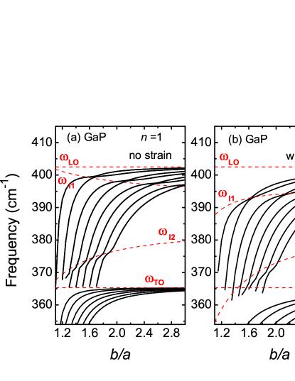
Figure 6: (Color online) GaP optical coupled phonon modes at $k_{z}=0$ for $n=1$ in GaAs-GaP core-shell nanowire as a function of the relation $\gamma=b/a$. Panel (a) neglecting strain, panel (b) considering strain effects. In the calculation we fixed the value of $a=3$ nm and $\varepsilon_{D}=2.56$. The bulk LO and TO phonon frequencies are indicated by dashed lines. The corresponding I-phonon frequencies obtained in the framework of the DCA are also represented by a gray (red) dashed line.

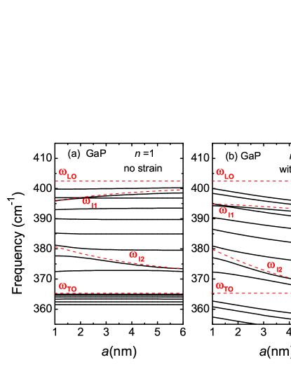
Figure 7: (Color online) The same as Fig. 6 but as a function of the core radius $a$, and fixing the value of $b-a=3$ nm.

Figure 7 displays the coupled shell modes at $k_{z}=0$ for $n=1$, as a function of the core radius. Notice that shell modes depend very weakly on the radius $a$ when strain effects are neglected. Only four modes close to the I-phonon do have a certain dispersion (see Fig. 7 (a)). When strain effects are taken into account, there is a general dependence in the core radius $a$ for all the modes due to mixing, Fig. 7(b). As we fixed $b-a=3$ nm, the shell modes remain confined even for very large core radius $a$. Moreover, the strain effect produces the shifts $\Delta\omega_{i}=-2\gamma_{i}\omega_{i}\varepsilon_{\mathrm{misfit}}(1-2\nu_{c})/(\nu_{c}-1)$ ($i=LO,TO$) to the longitudinal and transversal confined phonon frequencies.

VI.2 Modes with $k_{z}\neq 0$

Although we can obtain the general expressions for $k_{z}\neq 0$, the equations for the eigenmodes are so lengthy that we only give here those simpler case, with $n=0$. The form of the basis vectors (16) for $n=0$, $k_{z}\neq 0$ allows us to infer that the modes $T2$ are uncoupled from the rest.

VI.2.1 Core modes

The uncoupled transverse $T2$ modes for $n=0$ are given by $J_{1}(\mu^{(m)}_{1})=0$, which yields the equations for the eigenmodes $\omega_{T}^{2}=\left(\omega_{TO}+\Delta\omega_{TO}\right)^{2}-\beta_{T}^{2}\left((\mu^{(m)}_{1}/{a})^{2}-k^{2}_{z}\right)$, with $m=1,2,...$. This dispersion relation is equal to that of the bulk core material, save an energy shift given by the term $\left(\mu^{(m)}_{1}\beta_{T}/{a}\right)^{2}$, which takes into account the spatial confinement.

The system of equations for the $n=0$ coupled $L$-$T1$ core modes can be written in a rather compact form, as given in the Appendix (Eq. 92). From this expression, one can obtain the corresponding dispersion relations. We do not give the explicit equations for the $n=1$ modes, but we show here the numerical solutions corresponding to these phonon branches. Fig. 8(a) depicts the coupled $n=0$ core modes vs. $k_{z}$ for a range within a fifth of the first Brillouin zone of the bulk material, as obtained from Eq. (92). Fig. 8 (b) shows the core modes with $n=1$. In both cases we have considered strained core-shell nanowires.

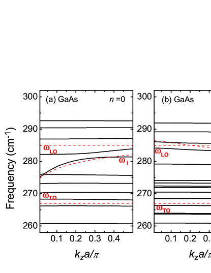
Figure 8: (Color online) Dispersion relations for the core modes of a core-shell GaAs-GaP nanowire. Panel (a) shows the coupled modes with $n=0$, panel (b) all modes with $n=1$. $LO$, $TO$ bulk and the $n=1$ interface phonon frequencies are shown with gray (red) dashed lines. Calculations are for $a=3$ nm and $b/a=2$.

VI.2.2 Shell modes

We give here the explicit equations for the simpler case, $n=0$. The $n=0$ shell transversal $T2$ eigenmodes are obtained from the equation

$$J_{1}(\mu_{1}^{(m)})N_{1}(\gamma\mu_{1}^{(m)})-J_{1}(\gamma\mu_{1}^{(m)})N_{1}(\mu_{1}^{(m)})=0,$$ (56)

which gives $\omega_{T}^{2}=\left(\omega_{TO}+\Delta\omega_{TO}\right)^{2}-\beta_{T}^{2}\left((\mu^{(m)}_{1}/{a})^{2}-k^{2}_{z}\right)$ with $m=1,2,...$, where $\mu_{1}^{(m)}$ represents the solutions of Eq. (56) for a given $\gamma$.

With respect to the coupled $L$-$T1$ shell modes, the corresponding system of equations, obtained from the boundary conditions for $n=0$, is given in the Appendix (Eq. 112). The solution of these equations yields the dispersion relations presented in Fig. 9(a); in panel (b) we also give the modes for $n=1$.

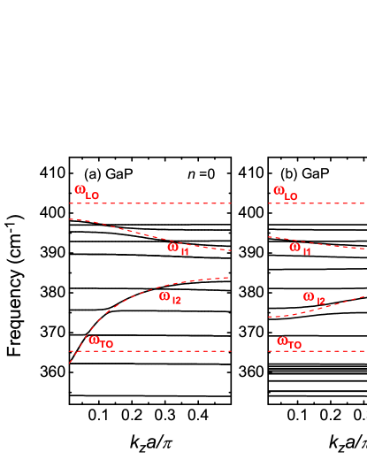
Figure 9: (Color online) Shell modes of a core-shell GaAs-GaP nanowire as a function of wave vector $k_{z}$. Panel (a) shows the coupled modes with $n=0$, panel (b) the $n=1$ modes. $LO$, $TO$ bulk and $n=1$ interface frequencies are shown with gray (red) dashed lines. Calculations are for fixed $a=3$ nm and $b/a=2$.

VII Conclusions

In this work we study the confined and interface polar optical phonons in core-shell nanowires by using a phenomenological continuum approach that takes into account the coupling of electromechanical oscillations and valid in the long-wave limit.

We derive a general analytical basis for the oscillations in cylindrical geometry with circular cross section, which allows for the obtention of polar vibrational properties in a variety of nanowire systems and materials, by the appropriate choice of boundary conditions. This permits an unambiguous identification of the coupled and uncoupled core and shell modes in terms of the phonon quantum numbers in these novel structures.

Our results for core and shell modes are summarized as follows. (i) There are uncoupled confined longitudinal and two transversal modes with $k_{z}=0$, $n=0$; (ii) we have found uncoupled confined transversal modes with $k_{z}=0$, $n=0,1,2..$ or $k_{z}\neq 0,n=0$; (iii) the modes with $k_{z}=0$,$n=0,1,2,...$, have a longitudinal and transversal mixed character, which couple the mechanical displacement vector $\vec{u}$ and the electrostatic potential $\varphi$; (iv) there are coupled longitudinal and two transversal modes for $k_{z}\neq 0,n\neq 0.$ We have also calculated the interface optical phonons in the framework of DCA, involving the electric potential of the phonon oscillations. We display the dispersion curves for the frequencies and compared both methods, i.e., the phenomenological continuum approach and the dielectric model. We have chosen the GaAs-GaP core-shell nanowire as an example system to apply our model, taking into account strain. We have found that the inclusion of strain is in fact crucial to model these nanowires, for their vibrational properties are modified dramatically by such strain effects. In particular, translationally invariant $(k_{z}=0$) core modes, which are independent of the shell radius when strain is neglected, acquire a dependence on the shell thickness if strain is included. In general, the inclusion of strain produces a shift on the core and shell modes. While for the core modes the frequencies have an upward shift, the shell modes present an important downshift of the spectra. Quantum confinement effects are important for smaller system sizes: when the core radius $a$ or the shell thickness $b-a$ are smaller than 3 nm, they become of the order of strain effects. In the core confinement effects have an opposite sign to those related to strain, whereas in the shell both have the same tendency.

One of the crucial results of the present work is straightforward implementation of the Fröhlich-like electron-phonon interaction Hamiltonian, $\widehat{H}_{F}=e\widehat{\varphi},$ for the core-shell nanowires. Using the general basic expression for the basis vectors (30) and employing Eqs. (43) with the appropriate boundary conditions (III), we are able to obtain the eigenfrequencies $\omega_{n,m,k_{z}}$ and the eigensolutions $F_{n,m,k_{z}}(\rho)\exp i(n\theta+k_{z}z)$, which fulfill the orthonormalization condition

$$\int\limits_{V}\rho_{M}(\rho)\vec{u}_{n,m,k_{z}}(\rho)\vec{u}_{n^{\prime},m,k_{z}}(\rho)\rho d\rho=\delta_{nn^{\prime}}.$$

Thus, we can construct the general solution for the displacement vector $\vec{u}(\rho,\theta,z)$ and the electrostatic potential $\varphi(\rho,\theta,z)$ which in second quantization read

$$\widehat{\vec{u}}=\sum\limits_{n,m,k_{z}}C_{n,m,k_{z}}\left[\vec{u}_{n,m,k_{z}}(\rho)\exp i(n\theta+k_{z}z)\widehat{b}_{n,m,k_{z}}+H.c.\right]$$

and

$$\widehat{\varphi}=\sum\limits_{n,m,k_{z}}C_{n,m,k_{z}}\left[\varphi_{n,m,k_{z}}(\rho)\exp i(n\theta+k_{z}z)\widehat{b}_{n,m,k_{z}}+H.c.\right],$$

where $\widehat{b}_{n,m,k_{z}}$ ($\widehat{b}_{n,m,k_{z}}^{\text{ }+})$ is the phonon annihilation (creation) operator and the $C_{n,m,k_{z}}$ coefficients are determined by the commutation rules $\left[\vec{u}(\vec{r}),\vec{\pi}(\vec{r}^{\prime})\right]=i\hbar\delta(r-r^{\prime})$ with $\vec{\pi}(\vec{r})$ being the momentum conjugate. Thus, it is possible to show that CTG92

$$C_{n,m,k_{z}}=\sqrt{\frac{\hbar}{2\omega_{n,m,k_{z}}}}$$

and the normalized Fröhlich interaction Hamiltonian can be cast as

$$\widehat{H}_{F}=\sum\limits_{n,m,k_{z}}e\sqrt{\frac{\hbar}{2\omega_{n,m,k_{z}}}}\left[\varphi_{n,m,k_{z}}(\rho)\exp i(n\theta+k_{z}z)\widehat{b}_{n,m,k_{z}}+C.C.\right].$$ (57)

In the same way, we can argue for the electron-phonon deformation potential interaction $\widehat{H}_{DP}.$ Notice that the procedure here implemented allows us to get the electron-phonon interactions that take into account the spatial confinement effect, the electrostatic influence on the phonon modes due the interfaces and the strain effect of the core-shell nanowires. Our work is relevant for the spectroscopic characterization of core-shell nanowires; it can be of interest for the experimental identification of these nanostructures.

Appendix A Secular equations for coupled modes

For the sake of completeness, we give here the lengthier systems of equations for coupled modes which were omitted in the main text.

The $L$-$T2$ shell modes for $n\neq 0$, $k_{z}=0$ are given by

$$\left(\begin{array}[]{cccccc}\frac{n}{t_{s}}J_{n}(t_{s})&\frac{n}{t_{s}}N_{n}(t_{s})&J^{\prime}_{n}(l_{s})&N^{\prime}_{n}(l_{s})&1&-1\\ J^{\prime}_{n}(t_{s})&N^{\prime}_{n}(t_{s})&\frac{n}{l_{s}}J_{n}(l_{s})&\frac{n}{l_{s}}N_{n}(l_{s})&1&1\\ \frac{n}{\gamma t_{s}}J_{n}(\gamma t_{s})&\frac{in}{\gamma t_{s}}N_{n}(\gamma t_{s})&J^{\prime}_{n}(\gamma l_{s})&N^{\prime}_{n}(\gamma l_{s})&\gamma^{n-1}&-\gamma^{-(n+1)}\\ J^{\prime}_{n}(\gamma t_{s})&N^{\prime}_{n}(\gamma t_{s})&\frac{in}{\gamma l_{s}}J_{n}(\gamma l_{s})&\frac{n}{\gamma l_{s}}N_{n}(\gamma l_{s})&\gamma^{n-1}&\gamma^{-(n+1)}\\ 0&0&S_{53}(l_{s})&S_{54}(l_{s})&S_{55}(t_{s})&S_{56}(t_{s})\\ 0&0&S_{63}(l_{s})&S_{64}(l_{s})&S_{65}(t_{s})&S_{66}(t_{s})\\ \end{array}\right)\left(\begin{array}[]{c}A^{(s)}_{T2}\\ B^{(s)}_{T2}\\ A^{(s)}_{L}\\ B^{(s)}_{L}\\ A^{(s)}_{H}\\ B^{(s)}_{H}\\ \end{array}\right)=\left(\begin{array}[]{c}0\\ 0\\ 0\\ 0\\ 0\\ 0\\ \end{array}\right)$$ (76)

with

$$S_{53}(l_{s}) = J^{\prime}_{n}(l_{s})-\frac{\varepsilon^{c}_{\infty}n}{\varepsilon^{s}_{\infty}l_{s}}J_{n}(l_{s}),S_{54}(l_{s})=N^{\prime}_{n}(l_{s})-\frac{\varepsilon^{c}_{\infty}n}{\varepsilon^{s}_{\infty}l_{s}}N_{n}(l_{s}),$$

$$S_{63}(l_{s}) = J^{\prime}_{n}(\gamma l_{s})+\frac{\varepsilon_{D}n}{\varepsilon^{s}_{\infty}\gamma l_{s}}J_{n}(\gamma l_{s}),S_{64}(l_{s})=N^{\prime}_{n}(\gamma l_{s})+\frac{\varepsilon_{D}n}{\varepsilon^{s}_{\infty}\gamma l_{s}}N_{n}(\gamma l_{s}),$$

$$S_{55}(t_{s}) = \frac{(\varepsilon^{c}_{\infty}-\varepsilon^{s}_{\infty})}{(\varepsilon^{s}_{0}-\varepsilon^{s}_{\infty})}\frac{(\omega^{2}_{TO}-\omega^{2})}{\omega^{2}_{TO}},S_{56}(t_{s})=-\frac{(\varepsilon^{c}_{\infty}+\varepsilon^{s}_{\infty})}{(\varepsilon^{s}_{0}-\varepsilon^{s}_{\infty})}\frac{(\omega^{2}_{TO}-\omega^{2})}{\omega^{2}_{TO}},$$

$$S_{65}(t_{s}) = -\frac{(\varepsilon_{D}+\varepsilon^{s}_{\infty})}{(\varepsilon^{s}_{0}-\varepsilon^{s}_{\infty})}\frac{(\omega^{2}_{TO}-\omega^{2})}{\omega^{2}_{TO}}\gamma^{n-1},S_{66}(t_{s})=\frac{(\varepsilon_{D}-\varepsilon^{s}_{\infty})}{(\varepsilon^{s}_{0}-\varepsilon^{s}_{\infty})}\frac{(\omega^{2}_{TO}-\omega^{2})}{\omega^{2}_{TO}}\gamma^{-(n+1)};$$

where $t_{s}=q_{T}a$, $l_{s}=q_{L}a$. In these parameters, as in $\omega_{TO}$, it is understood that shell values should be used.

We only give the equations for the dispersion relations, i.e., solutions for $k_{z}\neq 0$, for the $n=0$ coupled modes. The core $L$ -$T1$ coupled phonon bands are given by

$$\left(\begin{array}[]{ccccc}\frac{k_{a}}{l_{c}}J^{\prime}_{0}(t_{c})&J^{\prime}_{0}(l_{c})&I^{\prime}_{0}(k_{a})&0&0\\ -J_{0}(t_{c})&\frac{k_{a}}{l_{c}}J_{0}(l_{c})&I_{0}(k_{a})&0&0\\ 0&\frac{k_{a}}{l_{c}}J_{0}(l_{c})&-(1-\frac{\omega^{2}}{\omega^{2}_{TO}})I_{0}(k_{a})&\varepsilon^{c}_{\infty}I_{0}(k_{a})&\varepsilon^{c}_{\infty}K_{0}(k_{a})\\ 0&J^{\prime}_{0}(l_{c})&-(1-\frac{\omega^{2}}{\omega^{2}_{TO}})I^{\prime}_{0}(k_{a})&\varepsilon^{s}_{\infty}I^{\prime}_{0}(k_{a})&\varepsilon^{s}_{\infty}K^{\prime}_{0}(k_{a})\\ 0&0&0&C_{54}&C_{55}\\ \end{array}\right)\left(\begin{array}[]{c}A^{(c)}_{T1}\\ A^{(c)}_{L}\\ A^{(s)}_{H}\\ A^{(s)}_{H}\\ B^{(s)}_{H}\\ \end{array}\right)=\left(\begin{array}[]{c}0\\ 0\\ 0\\ 0\\ 0\\ \end{array}\right)$$ (92)

where

$$C_{54} = \varepsilon_{D}I_{0}(\gamma k_{a})K^{\prime}_{0}(\gamma k_{a})-\varepsilon^{s}_{\infty}I^{\prime}_{0}(\gamma k_{a})K_{0}(\gamma k_{a}),$$ (93)

$$C_{55} = (\varepsilon_{D}-\varepsilon^{s}_{\infty})K_{0}(\gamma k_{a})K^{\prime}_{0}(\gamma k_{a}).$$

The phonon dispersion relations for the $n=0$ coupled $L$-$T1$ shell modes can be obtained from

$$\left(\begin{array}[]{cccccc}\frac{k_{a}}{t_{s}}J^{\prime}_{0}(t_{s})&\frac{k_{a}}{t_{s}}N^{\prime}_{0}(t_{s})&J^{\prime}_{0}(l_{s})&N^{\prime}_{0}(l_{s})&I^{\prime}_{0}(k_{a})&K^{\prime}_{0}(k_{a})\\ -J_{0}(t_{s})&-N_{0}(t_{s})&\frac{k_{a}}{l_{s}}J_{0}(l_{s})&\frac{k_{a}}{l_{s}}N_{0}(l_{s})&I_{0}(k_{a})&K_{0}(k_{a})\\ \frac{k_{a}}{t_{s}}J^{\prime}_{0}(\gamma t_{s})&\frac{k_{a}}{t_{s}}N^{\prime}_{0}(\gamma t_{s})&J^{\prime}_{0}(\gamma l_{s})&N^{\prime}_{0}(\gamma l_{s})&I^{\prime}_{0}(\gamma k_{a})&K^{\prime}_{0}(\gamma k_{a})\\ -J_{0}(\gamma t_{s})&-N_{0}(\gamma t_{s})&\frac{k_{a}}{l_{s}}J_{0}(\gamma l_{s})&\frac{k_{a}}{l_{s}}N_{0}(\gamma l_{s})&I_{0}(\gamma k_{a})&K_{0}(\gamma k_{a})\\ 0&0&C_{53}&C_{54}&C_{55}&C_{56}\\ 0&0&C_{63}&C_{64}&C_{65}&C_{66}\\ \end{array}\right)\left(\begin{array}[]{c}A^{(s)}_{T1}\\ B^{(s)}_{T1}\\ A^{(s)}_{L}\\ B^{(s)}_{L}\\ A^{(s)}_{H}\\ B^{(s)}_{H}\\ \end{array}\right)=\left(\begin{array}[]{c}0\\ 0\\ 0\\ 0\\ 0\\ 0\\ \end{array}\right)$$ (112)

with

$$C_{53} = J^{\prime}_{0}(l_{s})I_{0}(k_{a})-\frac{\varepsilon^{c}_{\infty}}{\varepsilon^{s}_{\infty}}\frac{k_{a}}{l_{s}}J_{0}(l_{s})I^{\prime}_{0}(k_{a}),$$ (113)

$$C_{54} = N^{\prime}_{0}(l_{s})I_{0}(k_{a})-\frac{\varepsilon^{c}_{\infty}}{\varepsilon^{s}_{\infty}}\frac{k_{a}}{l_{s}}N_{0}(l_{s})I^{\prime}_{0}(k_{a}),$$

$$C_{55} = \frac{(\varepsilon^{c}_{\infty}-\varepsilon^{s}_{\infty})}{(\varepsilon^{s}_{0}-\varepsilon^{s}_{\infty})}\frac{(\omega^{2}_{TO}-\omega^{2})}{\omega^{2}_{TO}}I_{0}(k_{a})I^{\prime}_{0}(k_{a}),$$

$$C_{56} = \frac{(\omega^{2}_{TO}-\omega^{2})}{(\varepsilon^{s}_{0}-\varepsilon^{s}_{\infty})\omega^{2}_{TO}}(\varepsilon^{c}_{\infty}I^{\prime}_{0}(k_{a})K_{0}(k_{a})-\varepsilon^{s}_{\infty}I_{0}(k_{a})K^{\prime}_{0}(k_{a})),$$

$$C_{63} = J^{\prime}_{0}(l_{s})K_{0}(k_{a})-\frac{\varepsilon_{D}}{\varepsilon^{s}_{\infty}}\frac{k_{a}}{l_{s}}J_{0}(l_{s})K^{\prime}_{0}(k_{a}),$$

$$C_{64} = N^{\prime}_{0}(l_{s})K_{0}(k_{a})-\frac{\varepsilon_{D}}{\varepsilon^{s}_{\infty}}\frac{k_{a}}{l_{s}}N_{0}(l_{s})K^{\prime}_{0}(k_{a}),$$

$$C_{65} = \frac{(\omega^{2}_{TO}-\omega^{2})}{(\varepsilon^{s}_{0}-\varepsilon^{s}_{\infty})\omega^{2}_{TO}}(\varepsilon_{D}K^{\prime}_{0}(\gamma k_{a})I_{0}(\gamma k_{a})-\varepsilon^{s}_{\infty}K_{0}(\gamma k_{a})I^{\prime}_{0}(\gamma k_{a})),$$

$$C_{66} = \frac{(\varepsilon_{D}-\varepsilon^{s}_{\infty})}{(\varepsilon^{s}_{0}-\varepsilon^{s}_{\infty})}\frac{(\omega^{2}_{TO}-\omega^{2})}{\omega^{2}_{TO}}K_{0}(\gamma k_{a})K^{\prime}_{0}(\gamma k_{a}).$$

References

• (1) P. Yang, R. Yan, and M. Fardy, Nano Lett. 10, 1529 (2010).
• (2) B. Hua, J. Motohisa, Y. Kobayashi, S. Hara, and T. Fukui, Nano Lett. 9, 112 (2009).
• (3) Y. M. Niquet, Nano Lett. 7, 1105 (2007).
• (4) H.-M. Lin, Y.-L. Chen, J. Yang, Y.-C. Liu, K.-M. Yin, J.-J. Kai, F.-R. Chen, L.-C. Chen, Y.-F. Chen, and C.-C. Chen, Nano Lett. 3, 537 (2003).
• (5) M. Montazeri, M. Fickenscher, L. M. Smith, H. E. Jackson, J. Yarrison-Rice, J. H. Kang, Q. Gao, H. H. Tan, C. Jagadish, Y. Guo, J. Zou, M.-E. Pistol, and C. E. Pryor, Nano Lett. 10, 880 (2010).
• (6) L. Zhang and J.-jie Shi, Semicond. Sci. Tech. 20, 592 (2005).
• (7) P. K. Mohseni, A. D. Rodrigues, J. C. Galzerani, Y. A. Pusep, and R. R. LaPierre, J. Appl. Phys. 106, 124306 (2009).
• (8) M. F. Bailon-Somintac, J. J. Ibañez, R. B. Jaculbia, R. A. Loberternos, M. J. Defensor, A. A. Salvador, and A. S. Somintac, Journal of Crystal Growth 314, 268 (2011).
• (9) A. Giugni, G. Das, A. Alabastri, R. P. Zaccaria, M. Zanella, I. Franchini, E Di Fabrizio, and R. Krahne, Phys. Rev. B 85, 115413 (2012).
• (10) Y. Cui, Q. Wei, H. Park, and C. M. Lieber, Science 293, 1289 (2001).
• (11) G. Zheng, F. Patolsky, Y. Cui, W. Wang, and C. Lieber, Nature Biotechnology 23, 1294 (2005).
• (12) Y. Dong, B. Tian, T. J. Kempa, and C. M. Lieber, Nano Lett. 9, 2183 (2009).
• (13) E. D. Minot, F. Kelkensberg, M. van Kouwen, J. A. van Dam, L. P. Kouwenhoven, V. Zwiller, M. T. Borgström, O. Wunnicke, M. A. Verheijen, and E. P. A. M. Bakkers, Nano Lett. 7, 367 (2007).
• (14) A. Cros, R. Mata, K. Hestroffer, and B. Daudin, Appl. Phys. Lett. 102, 143109 (2013).
• (15) C. Trallero-Giner, R. Pérez-Alvarez, and F. García-Moliner, Long wave polar modes in semiconductor heterostructures, (Pergamon Elsevier Science, London, 1998).
• (16) M. A. Stroscio and M. Dutta, Phonons in nanostructures, (Cambridge University Press, Cambridge, 2001).
• (17) B.K. Ridley, Electrons and Phonons in Semiconductor Multilayers, (Cambridge University Press, Cambridge, 1997).
• (18) M. A. Stroscio, K. W. Kim, M. A. Littlejohn, and H. Huang, Phys. Rev. B 42, 1488 (1990).
• (19) R. Enderlein, Phys. Rev. B 47, 2162 (1993).
• (20) F. Comas, A. Cantarero, C. Trallero-Giner, and M. Moshinsky, J. Phys. Condens. Matter 7, 1789 (1995).
• (21) C. Trallero-Giner, F. García-Moliner, V. R. Velasco, and M. Cardona, Phys. Rev. B 45, 11944 (1992).
• (22) E. Roca, C. Trallero-Giner, and M. Cardona, Phys. Rev. B 49, 13704 (1994).
• (23) C. Trallero-Giner, Physica Scripta 55, 50 (1994).
• (24) F. Comas and C. Trallero-Giner, Philosophical Magazine, 70, 583 (1994).
• (25) P. M. Morse and H. Feshbach, Methods of Theoretical Physics, (McGraw-Hill, New York, 1953).
• (26) R. Ruppin and R. Englman, Rep. Prog. Phys. 33, 149 (1970).
• (27) M. Abramowitz and I. A. Stegun,  Handbook of Mathematical Functions with Formulas, Graphs, and Mathematical Tables, (Dover, New York, 1964).
• (28) L. Chico and R. Pérez-Álvarez, Phys. Rev. B 69, 035419 (2004).
• (29) L. Chico, R. Pérez-Álvarez, and C. Cabrillo, Phys. Rev. B 73, 075425 (2006).
• (30) F. Comas, C. Trallero-Giner, and A. Cantarero, Phys. Rev. B 47, 7602 (1993).
• (31) D. G. Santiago-Pérez, C. Trallero-Giner, R. Pérez-Álvarez, L. Chico, R. Baquero, and G. E. Marques, J. Appl. Phys. 112, 084322 (2012).
• (32) J. E. Spanier, R. D. Robinson, F. Zhang, S. W. Chan, and I. P. Herman, Phys.Rev. B 64, 245407 (2001).
• (33) Z. D. Dohcevic-Mitrovica, M. J. Scepanovica, M. U. Grujic-Brojcina, Z. V. Popovica, S. B. Boskovicb, B. M. Matovicb, M. V. Zinkevichc, and F. Aldinger, Solid State Commun 137, 387 (2006).
• (34) J. Menéndez, R. Singh, and J. Drucker, Ann. Phys. (Berlin) 523, 145 (2011).
• (35) W. Martienssen and H. Warlimont (Eds.), Springer Handbook of Condensed Matter and Materials Data, (Springer-Verlag, Berlin, 2005).
• (36) P. H. Borcherds, K. Kunc, G. F. Alfrey, R. L. Hall, J. Phys. C: Solid State Phys., Vol. 12 (1979).
• (37) S. Adachi, Properties of Group-IV, III-V and II-VI Semiconductors, (John Wiley and Sons, Chichester, 2005).