Multi-wavelength Hubble Space Telescope photometry of stellar populations in NGC 288.

Abstract

We present new UV observations for NGC 288, taken with the WFC3 detector on board the Hubble Space Telescope, and combine them with existing optical data from the archive to explore the multiple-population phenomenon in this globular cluster (GC). The WFC3’s UV filters have demonstrated an uncanny ability to distinguish multiple populations along all photometric sequences in GCs, thanks to their exquisite sensitivity to the atmospheric changes that are tell-tale signs of second-generation enrichment. Optical filters, on the other hand, are more sensitive to stellar-structure changes related to helium enhancement. By combining both UV and optical data we can measure helium variation. We quantify this enhancement for NGC 288 and find that its variation is typical of what we have come to expect in other clusters.

1 Introduction

Recent observations with the Hubble Space Telescope (HST) have shown that color-magnitude diagrams (CMDs) of globular clusters (GCs) are very different from our classical expectations of razor-thin sequences characteristic of single, old populations of stars. In particular, HST  near-UV data has shown that most, if not all, GCs host multiple stellar populations, as evidenced by two or more intertwined sequences in the CMD that we can trace from the main sequence (MS), through the sub-giant branch (SGB), up the red-giant branch (RGB) and even along the horizontal branch (HB).

¿From studies of several clusters, we have found that the different sequences can vary their color separation or even invert their relative colors, depending on the photometric-band combinations. These sequences correspond to stellar populations that have different abundances of light elements and helium. A comparison of the photometry with synthetic spectra can provide unique opportunities to estimate the helium content among the stellar populations (e.g. Milone et al. 2012a), even at the level of faint MS stars, which are unreachable by spectroscopic investigations.

The cluster analysed in this paper, NGC 288, is already known to host two populations of stars characterized by difference in light-element abundance (e.g. Shetrone & Keane 2000, Kayser et al. 2008, Smith & Langland-Shula 2009, Carretta et al. 2009, Pancino et al. 2010). The RGB of NGC 288 is bimodal, when observed in appropriate ultraviolet filters, and each RGB is populated by stars with different abundance of sodium and oxygen (Lee et al. 2009, Roh et al. 2011, Monelli et al. 2013).

In this paper, we combine new HST observations with archival data to investigate the evolutionary path of the multiple populations in NGC 288 along the MS, SGB, and RGB. By exploring a wide wavelength region, ranging from the ultraviolet ($\sim$2750Å) to the near infrared ($\sim$8140Å), we will estimate the helium difference between the two main populations.

2 Data and Data Reduction

To get the broadest possible perspective on NGC 288’s multiple populations, we consolidated photometry from a large number of HST images taken with the Wide Field Channel of the Advanced Camera for Surveys (ACS/WFC) and the ultraviolet/visible channel of the Wide-Field Camera 3 (WFC3/UVIS). Table 1 gives a list of the data sets we used. Most HST data are from the archive, with the exception of the proprietary images from GO-12605 (PI: Piotto), which were specifically taken for this project and are crucial for its success.

Photometric and astrometric measurements of ACS/WFC exposures were obtained with the software program described by Anderson et al. (2008). This routine produces a catalog of stars over the field of view by analyzing an entire set of images simultaneously. It measures stellar fluxes independently in each exposure by means of a spatially variable point-spread-function model (see Anderson & King 2006), along with a spatially-constant perturbation of the PSF to account for the effects of focus variations. The photometry has been calibrated as in Bedin et al. (2005), using the encircled energy and zero points of Sirianni et al. (2005).

The WFC3/UVIS images were reduced as described in Bellini et al. (2010), with
img2xym_UVIS_09$\times$10, a software routine that is adapted from img2xym_WFI (Anderson et al. 2006). Astrometry and photometry were corrected for pixel area and geometric distortion as in Bellini & Bedin (2009), and Bellini, Anderson & Bedin (2011). There are a few filters for which filter-specific distortion solutions are not yet available. For these filters (F395N, F467M, and F547M), we applied the solution for the closest available filter. This introduces small (0.05 pixel) errors in astrometry and negligible errors in photometry.

Since the main results of this paper require high-precision photometry, we limited our analysis to the sub-sample of stars well measured. The software routine provides several quality indexes that can be used as diagnostics of the reliability of photometric measurements: i) the rms of the individual position measurements about their mean, after they have been measured in different exposures and transformed into a common reference frame ($rms_{\rm X}$ and $rms_{\rm Y}$ ), ii) $o$, the ratio between the estimated flux of the star in a 0.5 arcsec aperture and the flux from neighbor stars that has spilled over into the same aperture), and iii) $q$, the residuals to the PSF fit for each star (see Anderson et al. 2008 for details). To select the high-quality sub-sample of stars we followed the approach described by Milone et al. (2009, Sect. 2.1). Photometry has been corrected for differential reddening by means of a procedure that has been adopted for several other projects and is described in detail in Milone et al. (2012b). Briefly, we define the fiducial MS for the cluster and then identify for each star a set of neighbors and determine from them their median offset relative to the fiducial sequence; this systematic color and magnitude offset, measured along the reddening line, is our estimate of the local differential-reddening value.

INSTR.	DATE	N$\times$EXPTIME	FILTER	PROGRAM	PI
ACS/WFC	Sep 20 2004	60s$+$680s	F435W	10120	S. Anderson
ACS/WFC	Sep 20 2004	10s$+$75s$+$115s$+$120s	F625W	10120	S. Anderson
ACS/WFC	Sep 20 2004	680s$+$1080s	F658N	10120	S. Anderson
ACS/WFC	Jul 31 2006	10s$+$4$\times$130s	F606W	10775	A. Sarajedini
ACS/WFC	Jul 32 2006	10s$+$4$\times$150s	F814W	10775	A. Sarajedini
WFC3/UVIS	Nov 11 2011	2$\times$360s	F547M	12193	J. W. Lee
WFC3/UVIS	Nov 11 2011	964s$+$1055s	F467M	12193	J. W. Lee
WFC3/UVIS	Nov 11 2011	1260s$+$1300s	F395N	12193	J. W. Lee
WFC3/UVIS	Oct 25 and Nov 7 2012	4$\times$400s$+$2$\times$401s	F275W	12605	G. Piotto
WFC3/UVIS	Oct 25 and Nov 7 2012	4$\times$350s	F336W	12605	G. Piotto
WFC3/UVIS	Oct 25 and Nov 7 2012	4$\times$41s	F438W	12605	G. Piotto

Table 1: List of the data sets used in this paper.

3 The color-magnitude diagram

A visual inspection of the CMDs that we obtain from the data sets listed in Tab. 1 indicates that the multiple populations along the MS, the RGB, and the SGB are best identified in the $m_{\rm F275W}$ versus $m_{\rm F275W}-m_{\rm F336W}$ and the $m_{\rm F275W}$ versus $m_{\rm F336W}-m_{\rm F438W}$ CMDs shown in Fig. 1. Panels (c) and (d) of the figure show a zoomed-in region around the MS and the RGB, and reveal, for the first time, that both the cluster MS and RGB are split into two sequences. Each sequence approximately contains the same number of stars. In the following, we will use for the two RGBs and MSs of NGC 288 the same nomenclature as previously adopted in our previous works for the cases of 47 Tuc (Milone et al. 2012a), NGC 6397 (Milone et al. 2012c), and NGC 6752 (Milone et al. 2013). In these papers we demonstrated that, in the $m_{\rm F275W}$ versus $m_{\rm F275W}-m_{\rm F336W}$ CMD, the blue- and the red-RGB stars are the progeny of blue- and red-MS stars, respectively. Here, for analogy, we indicate as MSa and RGBa the MS and RGB sequence with redder $m_{\rm F275W}-m_{\rm F336W}$ colors, while the bluer MS and RGB are named MSb and RGBb, respectively. The double SGB is highlighted in Fig. 1e. The two SGBs are well separated in color (by $\sim$0.05 mag) in the interval $-0.35<m_{\rm F336W}-m_{\rm F438W}<-0.15$, and then merge together at $m_{\rm F336W}-m_{\rm F438W}$$\sim-$0.15, with the faint SGB evolving into RGBa.

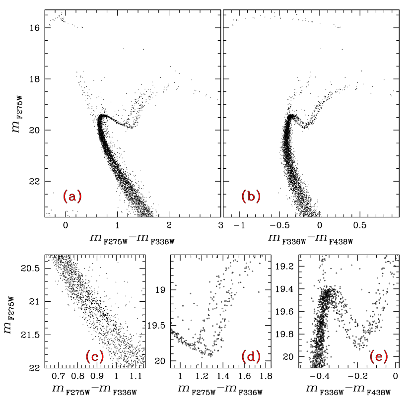
Figure 1: $m_{\rm F275W}$ versus $m_{\rm F275W}-m_{\rm F336W}$ (panel a) and $m_{\rm F275W}$ versus $m_{\rm F336W}-m_{\rm F438W}$ CMD (panel b) of NGC 288 after differential reddening correction. Panels (c), (d), and (e) are zoomed-in versions of panel (a) and (b) around the MS, RGB, and SGB, respectively.

3.1 Population ratio

In order to measure the fraction of stars in each MS, we followed the procedure illustrated in Fig. 2, again using techniques developed in previous studies (e.g. Piotto et al. 2007, 2012). The left panel shows the ${\it m}_{\rm F275W}$ vs. ${\it m}_{\rm F275W}-{\it m}_{\rm F336W}$ CMD of Fig. 1a, zoomed in around the MS region, in the interval 20.65$<m_{\rm F275W}<$23.2, where the bimodal distribution is most evident. The MS ridge line is marked in red. To determine it, we started by selecting a sample of MS stars by means of a hand-drawn, first-guess ridge line. We calculated the median color and the median magnitude of MS stars in bins that were 0.3 magnitude tall. We then interpolated these median points with a spline, and did an iterated sigma-clipping of the ’verticalized’ MS (middle panel). In order to obtain the ’verticalized’ MS of the middle panel, we subtracted from each star the color of the fiducial line at the same F275W magnitude level, obtaining a $\Delta$( $m_{\rm F275W}-m_{\rm F336W}$) value. The right panels of Fig. 2 show the histograms of the distribution of $\Delta$ ($m_{\rm F275W}-m_{\rm F336W}$) for six F275W magnitude intervals.

Finally, in each magnitude interval, we fit the histogram with a pair of Gaussians, colored green (for the redder peak) and magenta (for the bluer peak). Hereafter, these colors will be consistently used to distinguish the MSa and MSb populations and their post-MS progeny. From the areas under the Gaussians we estimate that 54$\pm$3% of the stars belong to the MSa and 46$\pm$3% to MSb. The errors were computed from the rms of the values obtained for the six intervals. In the WFC3/UVIS field of view, which includes the central part of the cluster with radial distance smaller than $\sim$1.2 core radii, the two MSs have almost the same number of stars in each magnitude interval, within the statistical uncertainties.

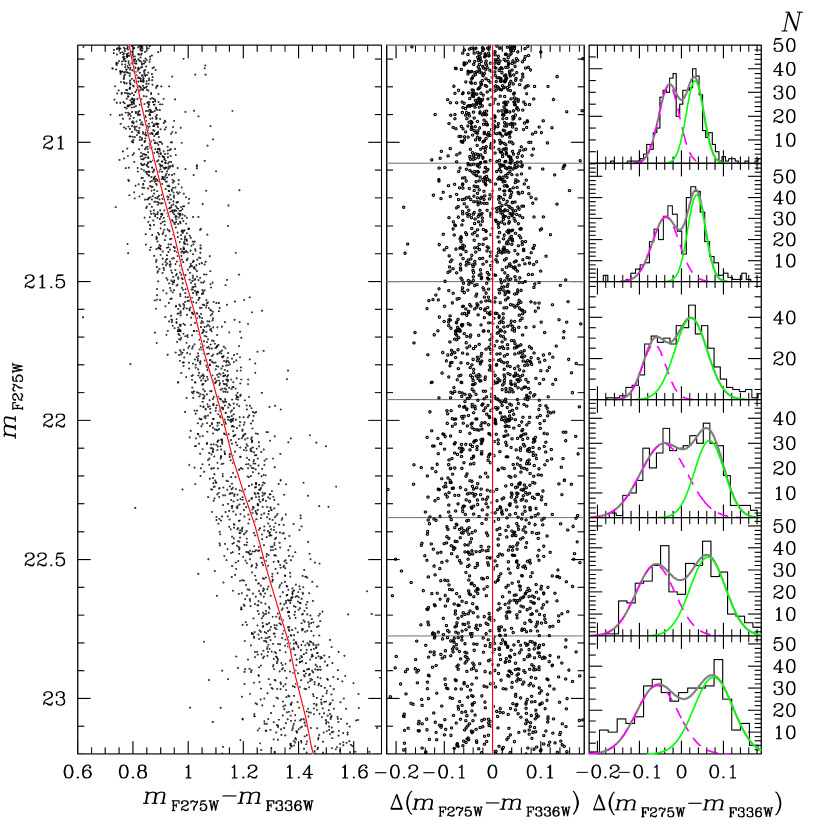
Figure 2: Left panel: CMD from Fig. 1a zoomed in around the MS region. The continuous line is a fiducial line for the MS. Middle panel: The same CMD, after subtraction of the color of the fiducial line. Right panels: Histograms of the $\Delta$ ($m_{\rm F275W}-m_{\rm F336W}$) distribution of the stars, in six magnitude intervals. The continuous gray lines show the best fit dual-Gaussian, composed by the sum of the magenta and green Gaussians.

In order to extend the study of stellar populations to the RGB and determine the fraction of RGBa and RGBb stars, in Fig. 3 we show the $m_{\rm F336W}-m_{\rm F438W}$ versus $m_{\rm F275W}-m_{\rm F336W}$ two-color diagram, where the RGB of NGC 288 is clearly split into two sequences. Here, we analyze only RGB stars with $m_{\rm F606W}<17.85$. Note that stars are selected on the basis of their F606W magnitude (in order to avoid any bias introduced to the strong luminosity difference between RGBa and RGBb stars in the ultraviolet filters). The red line is the hand-drawn fiducial line for the RGB. It separates RGBa stars (on the bottom-left side) from RGBb stars (on the upper-right side). We subtracted from the $m_{\rm F336W}-m_{\rm F438W}$ color of each star the corresponding color of the fiducial line, obtaining a $\Delta$($m_{\rm F336W}-m_{\rm F438W}$) index. The ’verticalized’ $m_{\rm F275W}-m_{\rm F336W}$ versus $\Delta$($m_{\rm F336W}-m_{\rm F438W}$) diagram is plotted in panel (b) of Fig. 3, while panel (c) shows the histogram of the $\Delta$($m_{\rm F336W}-m_{\rm F438W}$) distribution. The histogram is fitted with the sum of two Gaussians, again colored in green and magenta as above. From the area under the Gaussians we calculated that RGBa stars include 57$\pm$5% RGB stars, with the remaining 43$\pm$5% stars populating the RGBb. In this case, we simply associated a Poisson error to the fraction of stars in each population. Within one sigma uncertainty, these are the same fractions as for the MSa and MSb stars. From the weighted mean of the values obtained from the MS and RGB analysis, we obtain that population ‘a’ contains 55$\pm$3% and population ‘b’ the 45$\pm$3% of the total number of stars in the central region analyzed in this paper.

Our previous studies of 47 Tuc and NGC 6397 have demonstrated that any two-color diagram made from the combination of a near-ultraviolet filter (such as F225W or F275W), the F336W filter, and a blue filter (such as F390W, F435W, or F438W) is particularly efficient at disentangling stellar populations with different ligh-element abundances (Milone et al. 2012a, c). These photometric shifts can be interpreted in the light of spectroscopic observations.

Carretta et al. (2009) have analyzed GIRAFFE spectra of $\sim$130 stars, twenty-five of which are in common with the HST dataset of this paper. The spectroscopic targets are represented with large circles in Fig. 3 and are colored green and magenta according to their membership in the RGBa or the RGBb. The Na-O anticorrelation from Carretta and collaborators is reproduced in panel (d), while stars for which oxygen-abundance measurements are not available are arbitrarily plotted at the flagged value of [O/Fe]=0.85. The histogram distributions of [Na/Fe] for RGBa (green histogram) and RGBb stars (magenta histogram) are shown in panel (e). Similar to what is observed in the other GCs studied with a similar approach, we find that population ‘a’ stars are Na-poor and O-rich, in contrast to population ‘b’ stars, which are depleted in oxygen and enhanced in sodium.

Figure 3: Panel (a): $m_{\rm F275W}-m_{\rm F336W}$ versus $m_{\rm F336W}-m_{\rm F438W}$ two-color diagram for RGB stars. The continuous red line is the fiducial line for the RGB. Panel (b): Verticalized $m_{\rm F275W}-m_{\rm F336W}$ versus $\Delta$($m_{\rm F336W}-m_{\rm F438W}$) diagram. Panel (c): Histogram of the distribution of $\Delta$($m_{\rm F275W}-m_{\rm F336W}$) for the stars shown in the middle panel. The two components of the best-fitting dual-Gaussian function are colored green and magenta. Panel (d): Na-O anticorrelation for RGB stars by Carretta et al. (2009). Stars for which only sodium abundance are available are arbitrarily plotted at [O/Fe]=0.85 . In panels (a) and (d), RGBa and RGBb stars for which both spectroscopic and photometric measurements are available are plotted with green and magenta circles, respectively. Panel (e): Histogram of the [Na/Fe] distribution for RGBa (green) and RGBb stars (magenta).

3.2 A multiwavelength analysis of the double MS

By combining archive and proprietary data, we have access to eleven different photometric bands to build CMDs for NGC 288. We used the UV and blue photometry displayed in Figs. 1 to select the members of population ’a’ and ’b’, and then plotted their positions in the CMDs obtained with all possible color combinations. UV photometry has proven to be essential to separate the two populations, because of its sensitivity to light-element variations (Marino et al. 2008). On the other hand, optical CMDs are sensitive to He content and allow us to use the color separation of the CMD sequences (MS and RGB) to estimate their average helium difference. In particular, as shown by Sbordone et al. (2011), filters redder than F435W are marginally affected by differences in C N O abundances, while they are sensitive to the helium content of the two MSs.

Once we have selected the members of the two populations using the UV color-color diagrams, the optical photometry allows us to estimate the He content. Helium is extremely difficult to measure by spectroscopy in GC stars. Our procedure below is adapted from that in Milone et al.  (2013).

Fig. 4 shows the fiducial ridge lines for the MSa and MSb stars in the CMDs constructed with ${\it m}_{\rm F814W}$ vs. ${\it m}_{\rm X}-{\it m}_{\rm F814W}$ (where X= F275W, F336W, F395N, F435W, F438W, F467M, F547M, F606W, F625W, or F658N). A visual inspection reveals that MSa is generally redder than MSb, with the only exception of the ${\it m}_{\rm F814W}$ vs. ${\it m}_{\rm F336W}-{\it m}_{\rm F814W}$ baseline. The separation of the two sequences increases for larger color baselines in the remaining CMDs, in close analogy with what has been observed in the cases of $\omega$ Cen, NGC 6397, 47 Tuc, and NGC 6752.

Finally, we quantified the MS separation by measuring the color difference between MSa and MSb fiducials at a reference magnitude $m_{\rm F814W}^{\rm cut}$. We repeated this procedure for $m_{\rm F814W}^{\rm cut}=19.35,19.55,19.75,19.95,20.15$. As an example, we show the color differences for the case of $m_{\rm F814W}^{\rm cut}=19.75$ in Fig. 5 .

We followed the same procedure as used for the MS to analyze the color separation of RGBa and RGBb. Due to the relatively small number of RGB stars, we calculated the distance between the two RGB fiducials for the two values of $m_{\rm F814W}^{\rm cut}=17.25$ and $16.75$. In close analogy to the color behavior of the two MSs, RGBb is typically bluer than the RGBa, with the exception of CMDs based on the $m_{\rm F336W}-m_{\rm F814W}$ color. In the other filters the color distance from the RGBa of the RGBb increases with the color baseline. Results are illustrated in the right panel of Fig. 5 for $m_{\rm F814W}^{\rm cut}=16.75$.

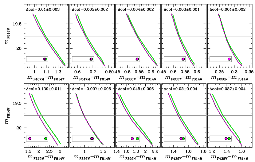
Figure 4: Color-magnitude diagrams for $m_{\rm F814W}$ versus $m_{\rm X}-m_{\rm F814W}$ for MSa (green lines) and MSb (magenta lines) fiducials (X= F275W, F336W, F395N, F435W, F438W, F467M, F547M, F606W, F625W, or F658N). At the top of each panel we give the color distance from the MSa, measured at $m_{\rm F814W}^{\rm cut}$=19.75 (solid line). The inset of each CMDs spans a total color interval of 0.17 mag and shows the relative positions of MSa and MSb represented as green and magenta circles, respectively, at $m_{\rm F814W}^{\rm cut}$=19.75.

Fig. 5 with synthetic photometry predictions. We used BaSTI isochrones (Pietrinferni et al. 2004, 2009) to calculate the surface temperature ($T_{\rm eff}$) and gravity ($\log g$) at different $m_{\rm F814W}$=$m_{\rm F814W}^{\rm cut}$ for two MS populations with helium abundances as listed in Table 2. Table 2 also gives the resulting ($T_{\rm eff}$) and gravity ($\log g$). In our calculation, we assumed $E(B-V)=0.03$ and $(m-M)_{\rm V}=14.84$ (Harris 1996, 2010 edition). We used the average [O/Fe] values for population ‘a’ and population ‘b’ stars derived by the measurements in Carretta et al. (2009): [O/Fe]=0.2 and [O/Fe]=$-$0.0 for first- and second-generation stars, respectively. Since neither carbon nor nitrogen abundance estimates were available for NGC 288, we arbitrarily assumed that the MSa has solar N and C, while MSb stars has a carbon depletion of 0.15 dex ([C/Fe]=$-0.15$) and enhanced in nitrogen by 0.7 dex ([N/Fe]=$+0.7$). To avoid the possibility that the adopted (and uncertain) values of [N/Fe] and [C/Fe] could affect our conclusions, we estimate helium only from filters redder than F435W. We assumed for the MSa primordial helium content (Y=0.246) and assumed for the MSb different helium abundances, with Y ranging from 0.246 to 0.300 in steps of $\Delta$Y=0.001.

We used the ATLAS12 program (Kurucz 2005, Castelli 2005, Sbordone et al. 2007) to account for the adopted chemical composition and performed spectral synthesis from $\sim$2,000 Å to $\sim$10,000 Å by using the SYNTHE code (Kurucz 2005). Synthetic spectra have been integrated over the transmission curves of the appropriated filters, and, for each value of Y of our grid, we calculated the color difference $m_{\rm X}-m_{\rm F814W}$.

The best fit between models and observations was determined by means of chi-square minimization. The helium difference corresponding to the best-fit models are listed in Table 2 for each adopted $m_{\rm F814W}^{\rm cut}$ value. From the average mean we obtain that population ‘b’ is helium-enhanced by $\Delta$Y=0.013$\pm$0.001, where the error is calculated from the agreement of the independent measurements. Results are shown in Fig. 5 for the case of $m_{\rm F814W}^{\rm cut}=19.75$, and $m_{\rm F814W}^{\rm cut}=16.75$. Models well match the data for the visual filters, while the agreement is poorer for the ultraviolet points, as expected since these baselines are very sensitive to C and N variations, and these abundances are not constrained by spectroscopy. A spectroscopic measure of the C and N for the two populations is clearly needed.

The C and N abundance differences between population ‘a’ and population ‘b’ stars that we arbitrarily adopted for NGC 288 are similar to those measured between first and second-generation stars of the GC M 4 and listed in Tab. 6 by Marino et al. (2008, see also Ivans et al. 1999, Villanova & Geisler 2011). In order to investigate the impact of our choice of C and N abundances on the inferred helium difference, we repeated the same procedure above by assuming that population ‘b’ stars are nitrogen enhanced by $\Delta$[N/H]=1.0 dex and carbon depleted by $\Delta$[C/H]=$-$0.5 dex with respect to population ‘a’ stars. In this case, the resulting $\Delta$Y is consistent with our previous estimate within 0.001 dex, indicating that the conclusions of this paper are not significantly affected by the choice of C and N.

Sequence	$m_{\rm F814W}^{\rm cut}$	$T_{\rm EFF}$ (Pop a)	$\log g$ (Pop a)	$T_{\rm EFF}$ (Pop b)	$\log g$ (Pop b)	Y (Pop a)	Y (Pop b)	$\Delta$Y
MS	19.35	6077	4.50	6100	4.49	0.248	0.262	0.014
MS	19.55	5966	4.54	5994	4.54	0.248	0.264	0.016
MS	19.75	5840	4.58	5861	4.58	0.248	0.259	0.011
MS	19.95	5701	4.62	5730	4.62	0.248	0.261	0.013
MS	20.15	5558	4.65	5583	4.65	0.248	0.259	0.011
RGB	16.75	5335	3.32	5347	3.31	0.248	0.265	0.017
RGB	17.25	5450	3.55	5463	3.54	0.248	0.260	0.012
AVERAGE						0.248	0.261	0.013$\pm$0.001

Table 2: Stellar parameters of the best-fitting model for population ‘a’ and population ‘b’ stars for different $m_{\rm F814W}^{\rm cut}$ values. The helium difference is listed in the last column, while the average $\Delta$Y is given in the list line.

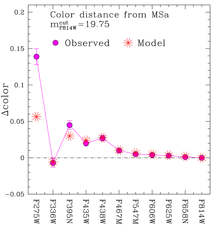
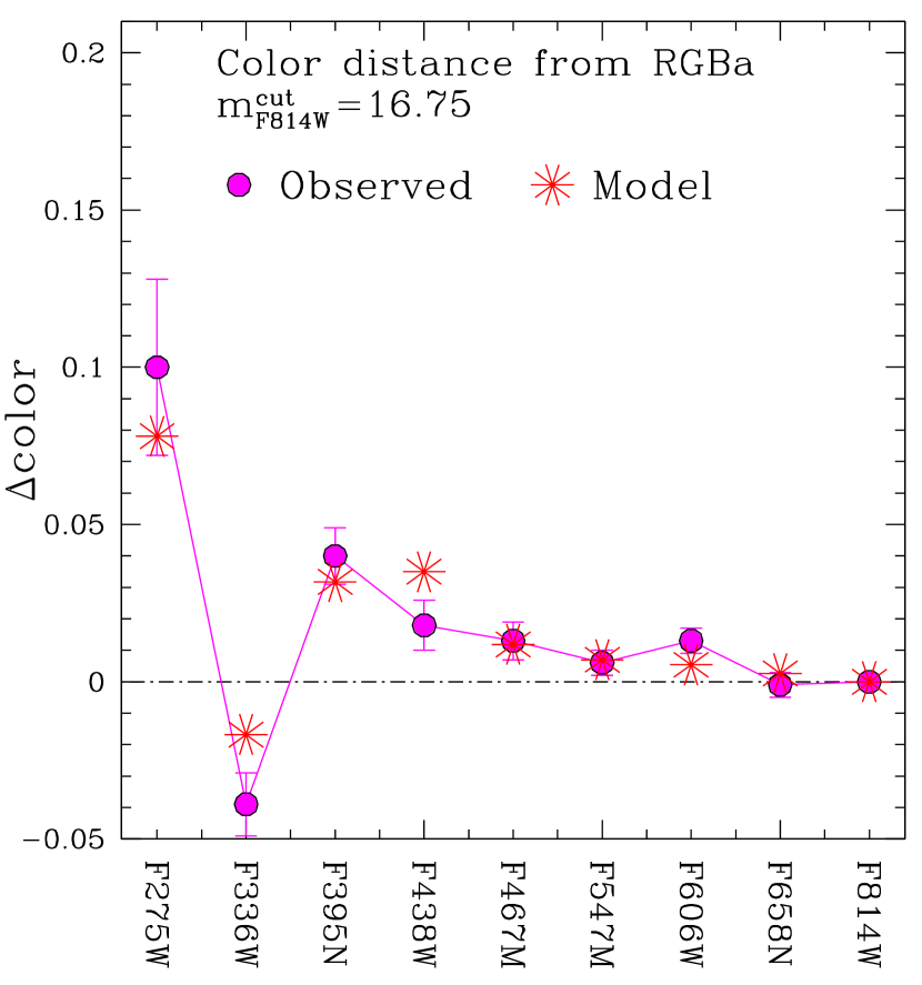
Figure 5: Observed $m_{\rm X}-m_{\rm F814W}$ color separation between MSa and MSb (left panel) and between RGBb and RGBa (right panel) for the available filters (magenta filled circles). Red asterisks indicate the synthetic colors corresponding to the best-fitting models. The color distances between the MS and RGB fiducials are measured at the reference magnitude $m_{\rm F814W}^{\rm cut}$=19.75, and $m_{\rm F814W}^{\rm cut}$=16.75, respectively.

4 Summary

We used multi-band HST photometry covering a wide range in wavelength to study the multiple stellar populations in NGC 288. Once again, UV photometry has proven essential to allow us to separate distinct stellar populations. For the first time, our photometry shows that this cluster’s MS splits into two branches, and we find that this duality is repeated along the SGB and the RGB, similar to what has been observed in other GCs. We calculated theoretical stellar atmospheres for main-sequence stars, assuming different chemical composition mixtures, and compared the predicted colors through the HST filters with our observed colors.

The observed color differences between the double MS and RGB of NGC 288 are consistent with two populations with different helium and light-element content. In particular, population ‘a’, which contains slightly more than half of the stars in NGC 288, corresponds to the first stellar generation with primordial He, and O-rich/Na-poor stars, while population ‘b’ is made of stars enriched in He by $\Delta Y=0.013\pm 0.001$ (internal error) and Na, but depleted in O. High-precision HST photometry allows us to estimate the He content difference at an accuracy beyond reach of spectroscopy.

References

- Anderson et al. (2006) Anderson, J., Bedin, L. R., Piotto, G., Yadav, R. S., & Bellini, A. 2006, A&A, 454, 1029
- Anderson & King (2006) Anderson, J., & King, I. R. 2006, Instrument Science Report ACS 2006-01, 34 pages, 1
- Anderson et al. (2008) Anderson, J., et al. 2008, AJ, 135, 2055
- Bedin et al. (2005) Bedin, L. R., Cassisi, S., Castelli, F., Piotto, G., Anderson, J., Salaris, M., Momany, Y., & Pietrinferni, A. 2005, MNRAS, 357, 1038
- Bellini & Bedin (2009) Bellini, A., & Bedin, L. R. 2009, PASP, 121, 1419
- Bellini et al. (2010) Bellini, A., Bedin, L. R., Piotto, G., Milone, A. P., Marino, A. F., & Villanova, S. 2010, AJ, 140, 631
- Bellini et al. (2011) Bellini, A., Anderson, J., & Bedin, L. R. 2011, PASP, 123, 622
- Carretta et al. (2009) Carretta, E., et al. 2009, A&A, 505, 117
- Castelli (2005) Castelli, F. 2005, Memorie della Societa Astronomica Italiana Supplementi, 8, 25
- Harris (1996) Harris, W. E. 1996, AJ, 112, 1487
- Harris (2010) Harris, W. E. 2010, arXiv:1012.3224
- Kayser et al. (2008) Kayser, A., Hilker, M., Grebel, E. K., & Willemsen, P. G. 2008, A&A, 486, 437
- Kurucz (2005) Kurucz, R. L. 2005, Memorie della Societa Astronomica Italiana Supplementi, 8, 14
- Ivans et al. (1999) Ivans, I. I., Sneden, C., Kraft, R. P., et al. 1999, AJ, 118, 1273
- Lee et al. (2009) Lee, J.-W., Kang, Y.-W., Lee, J., & Lee, Y.-W. 2009, Nature, 462, 480
- Marino et al. (2008) Marino, A. F., Villanova, S., Piotto, G., Milone, A. P., Momany, Y., Bedin, L. R., & Medling, A. M. 2008, A&A, 490, 625
- Milone et al. (2009) Milone, A. P., Bedin, L. R., Piotto, G., & Anderson, J. 2009, A&A, 497, 755
- Milone et al. (2012) Milone, A. P., Piotto, G., Bedin, L. R., et al. 2012, A&A, 540, A16
- Milone et al. (2012) Milone, A. P., Piotto, G., Bedin, L. R., et al. 2012, A&A, 540, A16
- Milone et al. (2012) Milone, A. P., Marino, A. F., Piotto, G., et al. 2012, ApJ, 745, 27
- Milone et al. (2013) Milone, A. P., Marino, A. F., Piotto, G., et al. 2013, ApJ, 767, 120
- Monelli et al. (2013) Monelli, M., Milone, A. P., Stetson, P. B., et al. 2013, MNRAS, 1005
- Pancino et al. (2010) Pancino, E., Rejkuba, M., Zoccali, M., & Carrera, R. 2010, A&A, 524, A44
- Pietrinferni et al. (2004) Pietrinferni, A., Cassisi, S., Salaris, M., & Castelli, F. 2004, ApJ, 612, 168
- (25) Pietrinferni, A., Cassisi, S., Salaris, M., Percival, S., & Ferguson, J. W. 2009, ApJ, 697, 275
- Piotto et al. (2007) Piotto, G., Bedin, L. R., Anderson, J., et al. 2007, ApJ, 661, L53
- Piotto et al. (2012) Piotto, G., Milone, A. P., Anderson, J., et al. 2012, ApJ, 760, 39
- Roh et al. (2011) Roh, D.-G., Lee, Y.-W., Joo, S.-J., et al. 2011, ApJ, 733, L45
- Sbordone et al. (2007) Sbordone, L., Bonifacio, P., & Castelli, F. 2007, IAU Symposium, 239, 71
- Sbordone et al. (2011) Sbordone, L., Salaris, M., Weiss, A., & Cassisi, S. 2011, A&A, 534, A9
- Shetrone & Keane (2000) Shetrone, M. D., & Keane, M. J. 2000, AJ, 119, 840
- Sirianni et al. (2005) Sirianni, M., et al. 2005, PASP, 117, 1049
- Smith & Langland-Shula (2009) Smith, G. H., & Langland-Shula, L. E. 2009, PASP, 121, 1054
- Villanova & Geisler (2011) Villanova, S., & Geisler, D. 2011, A&A, 535, A31