A State-Space Approach for Optimal Traffic Monitoring
via Network Flow Sampling

Abstract

The robustness and integrity of IP networks require efficient tools for traffic monitoring and analysis, which scale well with traffic volume and network size. We address the problem of optimal large-scale flow monitoring of computer networks under resource constraints. We propose a stochastic optimization framework where traffic measurements are done by exploiting the spatial (across network links) and temporal relationship of traffic flows. Specifically, given the network topology, the state-space characterization of network flows and sampling constraints at each monitoring station, we seek an optimal packet sampling strategy that yields the “best” traffic volume estimation for all flows of the network. The optimal sampling design is the result of a concave minimization problem; then, Kalman filtering is employed to yield a sequence of traffic estimates for each network flow. We evaluate our algorithm using real-world Internet2 data.

1 Introduction

Advances in networking technologies and high performance computing have led to an unprecedented growth of a vast array of applications such as cloud computing, social networking, video on demand, cloud storage, and voice over IP, to name a few. At the same time, malicious network activity remains a big concern since network attacks become more sophisticated. Therefore, it is extremely important for network operators to have an accurate global-view of their network for diagnosing anomalous activity [19], for optimal network capacity planning and quality of service considerations [5]. These can be achieved through network monitoring. However, monitoring everywhere and constantly is expensive, energy inefficient and computationally challenging. Thus, one should employ statistical tools for traffic estimation through limited collection of measurements.

Network monitoring has traditionally been done with SNMP measurements [5, 23, 32]. SNMP measurements provide link counts which give the aggregate traffic volume at the observation point of interest. Recently, more granularity can be achieved by performing flow-level measurements using tools such as Cisco’s NetFlow. The latter approach simplifies the monitoring task significantly. The idea is to sample packets from flows of interests at specific router interfaces, henceforth called observation points. For each packet sampled, several header information can be extracted and recorded for further analysis. Each packet from a flow (a flow can be an aggregate flow, i.e., flows originating from a particular subnet or an autonomous system) is sampled independently with a particular sampling probability (also known as sampling rate). Typical sampling rates are between $0.01$ (i.e., only 1 out of 100 packets is selected for sampling) and $0.20$. Higher sampling rates can also be chosen, but they amount to valuable resource consumption at each router (cache memory, CPU cycles, storage, network bandwidth and power). Thus, judicious choice of the sampling rates greatly affects the efficient operation of the network.

Regardless of the measurement technique, network monitoring aims to several objectives: a) identification of the traffic volume for network flows (known as traffic matrix) [26, 21, 23, 32, 27, 13], i.e., traffic for each origin-destination pair given the link counts and the topology of the network, b) identification of flow characteristics such as end-to-end network delay [4, 20, 6], flow length, flow distribution or other flow statistics [31, 10, 12]. To accomplish these, several interesting problems arise, such as the subset selection problem for choosing the locations of the monitoring stations [4, 6] and the sampling design problem [26].

This paper aims to address the problem of flow estimation through an optimal sampling strategy under resource constraints (see also [11]). We assume that network monitoring is performed via Netflow-alike measurements. Our framework takes into account both temporal correlations of the flows (see also [13]) as well as their spatial correlation [14]. We adapt Bernoulli sampling for our measurements at each observation site (that is, the information of a packet at each network link is recorded according to the sampling rate/probability described above), but alternative sampling techniques can aslo be considered [8, 7, 9].

The toy-example of Figure 1 provides more insights on the proposed method; assume we have flows between each network node. Further, assume flow-monitoring tools can sample with rate $20$ out of every $100$ packets. How should the network operator assign the sampling rates to each flow subject to the sampling capacity of each link? By considering the network topology, one would expect that “long-flows” do not require many samples at every single link they traverse. For example, the flow from ’Houston’ to ’NY’ needs not be sampled at every link on its path. Sampling on link ’Houston’ - ’Kansas’ may be sufficient; this will leave the resources of the intermediate link to be utilized for monitoring the “short” flow that traverses only the link ’Kansas’ to ’Chicago’. Similarly, a stochastic characterization of the “evolution” of each flow over time provides valuable information for choosing the “’best” sampling strategy. Section 2 unifies these ideas in a stochastic optimization framework.

Similar approaches for flow estimation via state-space models have also appeared in [26, 27]. However, in [26] the proposed method addresses flow estimation on a single network link and the spatial correlation between flows are not examined. In [27], the suggested state-space model considers link counts at every network link without relying on flow sampling (in particular, SNMP counts are considered). In large-scale networks this approach is not practical nor feasible. Further, compared to [27], we study a framework better-tailored to the ongoing measurement process.

The contributions of this paper are twofold: a) We present a stochastic optimization framework for finding the optimal sampling design that would yield the best traffic estimates for each flow (section 2). The model views each flow as a stochastic process. The state of the system at a particular time instance is the volume of traffic that each flow carries at that instance. Through sampling, we get a partially observed system; this observation uncertainty is captured through the measurement equations we define next. The goal is to find the “best” sampling strategy that minimizes the estimation error over the (finite) horizon of interest. This is the first attempt to model the flow estimation problem under a stochastic control framework; b) We study an approximation scheme for the solution of the above-mentioned stochastic optimization problem (section 3). The problem of obtaining the optimal sampling rates is then reduced to a deterministic optimization problem that can be solved a priori. Based on the calculated sampling rates, traffic estimation for each time-step is then performed via the Kalman filter. As illustrated in Figure 2 the proposed approach poses significant gains over existing techniques. We evaluate our approach using real-world data obtained from Internet2 (section 4).

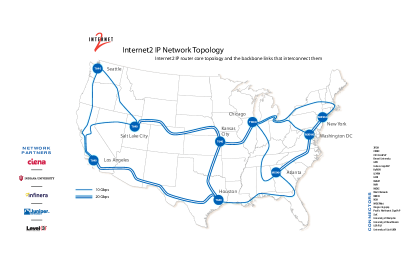
Figure 1: Backbone network of Internet2.

2 Problem Description

Consider a communication network of $N$ nodes and $L$ links. The total number of traffic flows, i.e. source and destination $(S,D)$ pairs, is denoted by $J$. We denote the set of flows as $\mathcal{J}:=\{1,2,\ldots,J\}$ and the set of all network links with $\mathcal{L}:=\{1,2,\ldots,L\}$. Traffic is routed over the network along predefined paths described by a routing matrix $R=(r_{\ell,j})_{L\times J},$ with $r_{\ell,j}=1,\mbox{when route $j$ uses link $\ell$ }$ and $0$ otherwise. Let

$$\mathbf{x}_{t}=(x_{t}(1),x_{t}(2),\ldots,x_{t}(J))^{T},t=1,2,\ldots$$

and

$$\mathbf{y}_{t}=(y_{t}(1),y_{t}(2),\ldots,y_{t}(L))^{T},t=1,2,\ldots$$

be the vector time series of traffic traversing all $J$ routes and $L$ links, respectively. We shall ignore network delays and adopt the assumption of instantaneous propagation. This is reasonable when traffic is monitored at a time-scale coarser than the round-trip time of the network, which is the case in our setting. We thus obtain that the link and route level traffic are related through the fundamental routing equation

$$\mathbf{y}_{t}=R\mathbf{x}_{t}.$$ (1)

The spatial correlation between flows encoded in the routing matrix $R$, will play an important role in determining the optimal sampling design. Before discussing the solution of our optimization problem though, we first consider in detail all the components of our stochastic control formulation.

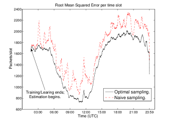
Figure 2: Estimation error per time interval: comparison of optimal versus naïve sampling for the $72$ Internet2 flows on 2009-03-17.

2.1 A State-Space Model

In this paper, we model the evolution over time of the volume of each flow as a stochastic process. In particular, we model the dynamics of each flow $j,j=1,2,\ldots,J$, as the following Markov process:

$$x_{t+1}(j)=\rho_{j}x_{t}(j)+w_{t}(j),t=0,1,2,\ldots$$ (2)

where $x_{t}(j)$ represents the state of flow $j$ at time $t$, namely the numbers of packets (or bytes) carried at time interval $t$. For the purposes of this paper we assume that each time interval has a duration of $10$ minutes. The sequence of random variables $w_{t}(j),t=1,2,\ldots$ represent random noise. They belong to the set of primitive random variables, meaning that they are mutually independent. They are also independent from the state random variables. We assume noise to be Gaussian with zero mean and variance equal to $\sigma_{\epsilon}^{2}$. To fully characterize the system evolution for flow $j$ of Eq. (2) we need initial state $x_{0}(j)$, which is also assumed to be Gaussian. Its mean and variance can be calculated during a calibration phase. To summarize, for $t=0,1,2,\ldots$, the system dynamics are described by

$$\mathbf{x}_{t+1}=F\mathbf{x}_{t}+\mathbf{w}_{t},$$ (3)

with $\mathbf{x}_{t}$ being the vector representing the “state” of each flow at time $t$, and $F$ a diagonal matrix of the coefficients $\rho_{j}$. Moreover, we have the following probability density functions for the primitive random variables described above, i.e.,

$$p(\mathbf{x}_{0}) =c_{1}{\rm exp}\{-\frac{1}{2}[(\mathbf{x}_{0}-\mathbf{\bar{x}_{0}})^{T}(\hat{P}_{0|-1})^{-1}(\mathbf{x}_{0}-\mathbf{\bar{x}_{0}})]\}$$ (4)

$$p(\mathbf{w}_{t}) =c_{2}{\rm exp}\{-\frac{1}{2}[\mathbf{w}_{t}^{T}\hat{Q}^{-1}\mathbf{w}_{t}]\}.$$ (5)

The parameters $\mathbf{x}_{0}$, $\hat{P}_{0|-1}$, $F$ and ${\hat{Q}}$ can be determined through a short calibration phase using techniques for fitting autoregressive models (see [3], Chapter 8).

2.2 Traffic Measurement

2.2.1 Bernoulli flow sampling

As mentioned above, at time $t$ the volume of flow $j$ is denoted by the state variable $x_{t}(j)$. We adopt a Bernoulli sampling scheme [12]. This says that each packet of flow $j$ passing through the observation point $\ell$ at time $t$, is sampled with probability $u_{t}(\ell,j)$. In other words, the variable $u_{t}(\ell,j)$ specifies the sampling rate at link $\ell$ for flow $j$ at time $t$.

The number of packets captured at observation point $\ell$ for flow $j$ is given by the random variable $\tilde{y}_{t}(\ell,j)$. Given $x_{t}(j)$, $\tilde{y}_{t}(\ell,j)$ follows a binomial distribution, i.e.,

$$\tilde{y}_{t}(\ell,j)\sim\rm{Binomial}(x_{t}(j),u_{t}(\ell,j)).$$ (6)

Based on the observations $\tilde{y}_{t}(\ell,j)$, the unbiased estimator for $x_{t}(\ell,j)$ – the traffic volume at link $\ell$ for flow $j$ – is given by:

$$\tilde{z}_{t}(\ell,j)=\frac{\tilde{y}_{t}(\ell,j)}{u_{t}(\ell,j)}.$$ (7)

The variance of the estimator at link $\ell$ for flow $j$ equals

$$v_{t}(\ell,j):= \mathbb{E}[(\tilde{z}_{t}(\ell,j)-\mathbb{E}\tilde{z}_{t}(\ell,j))^{2}|{x_{t}(j)}]$$

$$= \mathbb{E}[(\tilde{z}_{t}(\ell,j)-x_{t}(j))^{2}|x_{t}(j)]$$

$$= x_{t}(j)\frac{1-u_{t}(\ell,j)}{u_{t}(\ell,j)}.$$ (8)

2.2.2 Spatial combination of estimators

We seek a combined estimator for the volume of flow $j$ that uses measurements from several observation points [14]. Such an estimator can be expressed as,

$$z_{t}(j)=\sum_{\ell\in\ell(j)}w_{\ell,j}\tilde{z}_{t}(\ell,j),$$ (9)

where $\ell(j)\subseteq\mathcal{L}$ is the set of links that flow $j$ traverses. Conditioned on the state $x_{t}(j)$, the observations at different links $\tilde{y}_{t}(\ell,j)$ are independent so one can calculate the variance of the combined estimator to be

$$\rm{Var}(z_{t}(j)|x_{t}(j))=\sum_{\ell\in\ell(j)}{w^{2}_{\ell,j}}v_{t}(\ell,j),$$ (10)

where $v_{t}(\ell,j)=x_{t}(j)\frac{1-u_{t}(\ell,j)}{u_{t}(\ell,j)}$ (see Eq. (2.2.1)) and $\ell(j)$ is the set of links that flow $j$ is traversing and can be acquired from the routing matrix $R$. To obtain the best linear unbiased estimator for all $j\in\mathcal{J}$, we want to find the optimal weights $w_{\ell,j}$ that minimize the above variance subject to $\sum_{\ell\in\ell(j)}w_{\ell,j}=1$. Taking the Lagrangian and using the first-order optimality conditions we arrive to

$$w_{\ell,j}=\frac{v_{t}(\ell,j)^{-1}}{\sum_{k\in\ell(j)}v_{t}(k,j)^{-1}}.$$ (11)

Continuing from (10),

$$\rm{Var}(z_{t}(j)|x_{t}(j))=\frac{1}{\sum_{k\in\ell(j)}\frac{1}{v_{t}(k,j)}}.$$ (12)

2.2.3 The Measurement Equation

From Eqs. (6), (7), (9) we see that we have a partially observable system. In other words, the state $\mathbf{x}_{t}$ of the system – the traffic volume for each flow at $t$ – is not directly available, but can be inferred through the observations $\mathbf{z}_{t}$. Using the normal approximation to the binomial distribution we get the following relation between the state and observations for flow $j$, for $t=1,2,\ldots$

$$z_{t}(j)=x_{t}(j)+r_{t}(j),$$ (13)

where $r_{t}(j)$ is a Gaussian random variable, i.e. (see Eq. (12))

$$r_{t}(j) \sim\mathcal{N}\Big{(}0,\frac{x_{t}(j)}{\sum_{k\in\ell(j)}\frac{1}{\frac{1}{u_{t}(k,j)}-1}}\Big{)}$$ (14)

The measurement equation, for all flows becomes

$$\mathbf{z}_{t}=\mathbf{x}_{t}+\mathbf{r}_{t},$$ (15)

with the probability density function for $\mathbf{r}_{t}$ being

$$p(\mathbf{r}_{t}) =c_{3}{\rm exp}\{-\frac{1}{2}[\mathbf{r}_{t}^{T}\hat{R}_{t}(\mathbf{x}_{t},\mathbf{u}_{t})^{-1}\mathbf{r}_{t}]\},$$ (16)

where $\hat{R}_{t}(\mathbf{x}_{t},\mathbf{u}_{t})$ is a covariance matrix. Using the proposed measurement scheme, the covariance matrix is just a diagonal matrix with elements the variances shown in Eq. (14).

2.3 The Instantaneous Cost

Let $\mathbf{u}_{t}\in(0,1)^{L\times J}$ be the sampling matrix arranged in a vector form; the variable $u_{t}(\ell,j)$ specifies the sampling rate at link $\ell$ for flow $j$ at time $t$. We define the instantaneous cost to be the estimation error at time $t$ as follows:

$$c_{t}({\mathbf{x}_{t}},\mathbf{u}_{t}):={\rm{trace}}\Big{(}\mathbb{E}[(\mathbf{z}_{t}-\mathbf{x}_{t})(\mathbf{z}_{t}-\mathbf{x}_{t})^{T}]\Big{)},$$ (17)

where $\mathbf{z}_{t}:=\mathbf{z}_{t}(\mathbf{u}_{t})$ is the vector of volume estimation for each flow $j=1,2,\ldots J$ at time $t$ (see Eq. (9) and (11)).

The instantaneous cost of (17) can then be written as:

$$c_{t}({\mathbf{x}_{t}},\mathbf{u}_{t})=\sum_{j=1}^{J}\frac{1}{\sum_{k\in\ell(j)}\frac{1}{v_{t}(k,j)}}.$$ (18)

Proposition 1

The instantaneous cost function shown in (18) is concave in $\mathbf{u_{t}}$.

Proof 2.1.

Using the expanded form of Eq. (18) with $v_{t}(k,j)=x_{t}(j)(\frac{1}{u_{t}(k,j)}-1)$ we observe that this resembles the harmonic average of the terms $v_{t}(k,j)$. Using the fact that the harmonic average function is a concave and non-decreasing function [2], one can easily verify that our objective function is concave in $\mathbf{u_{t}}$ as a composition of a concave and non-decreasing function with a convex function.

3 Optimal Sampling

The problem at hand belongs to the category of measurement adaptive problems [30]. In the general case, the problem of optimal measurement control (see also sequential design of experiments [25]) can be formulated as the following discrete-time, finite-horizon, partially-observable, perfect-recall stochastic control problem (see [30, 18]).

We are given, the system evolution equation, written as

$$\mathbf{x}_{t+1}=f_{t}(\mathbf{x}_{t},\mathbf{w}_{t}),t=0,1,2,\ldots,T,$$ (19)

the measurement equation

$$\mathbf{z}_{t}=h_{t}(\mathbf{x}_{t},\mathbf{u}_{t},\mathbf{r}_{t}),t=0,1,2,\ldots,T,$$ (20)

and the probability densities for the random variables $\mathbf{x}_{0}$, $\mathbf{w}_{t}$ and $\mathbf{r}_{t}$

$$p(\mathbf{x}_{0}),p(\mathbf{w}_{t}),p(\mathbf{r}_{t}),t=0,1,2,\ldots,T.$$ (21)

The performance criterion is the expected cost over the horizon of interest

$$V=\mathbb{E}\{\sum_{t=0}^{T-1}c_{t}(\mathbf{x}_{t},\mathbf{u}_{t})+c_{T}(\mathbf{x}_{T},\mathbf{u}_{T})\},$$ (22)

where $c_{t}(\mathbf{x}_{t},\mathbf{u}_{t})$ is the instantaneous cost function and the expectation is taken with respect to the random variables $\mathbf{x}_{t}$.

The problem is to find the optimal sampling strategy

$$g:=(g_{1}(\mathbf{Z}^{1}),\ldots,g_{t}(\mathbf{Z}^{t}),\ldots,g_{T}(\mathbf{Z}^{T}))$$

that minimizes the expected cost (22) over the horizon of interest subject to “budgetary” sampling constraints. The symbol

$$\mathbf{Z}^{t}:=(\mathbf{z}_{1},\mathbf{z}_{2},\dots,\mathbf{z}_{t}),$$ (23)

represents the history of observations up to time $t$. Simi-larly, the history of sampling rates up to time $t$ will be denoted as $\mathbf{u}^{t}$. As mentioned above, we assume a system with perfect-recall which means that all this information is available. Having calculated an optimal sampling strategy, the optimal sampling action at time instance $t$ would be

$$\mathbf{u}_{t}=g_{t}(\mathbf{Z}^{t}).$$ (24)

In other words, given the history of observations, the optimal action would at time $t$ will be given by the pre-calculated optimal policy.

In the general case, applying dynamic programming is hindered by the curse of dimensionality [24]. Therefore, some sort of approximation techniques need to be involved [24, 1]. Indeed, under the following conditions, the stochastic control problem can be solved efficiently [22] by exploiting the two-way separation between estimation and control [30, 18]. The conditions are: a) The system evolution equation (see Eq. (19)) is linear; b) The measurement equation (see Eq. (20)) is linear in the state and measurement noise; c) The primitive random variables are Gaussian; and d)The instantaneous cost (in our case given by Eq. (17)) is independent of the state $\mathbf{x}_{t}$.

In the special case we have a state equation of the following form

$$\mathbf{x}_{t+1}=F_{t}\mathbf{x}_{t}+\mathbf{w}_{t},$$ (25)

a measurement equation of this form

$$\mathbf{z}_{t}=H_{t}(\mathbf{u}_{t})\mathbf{x}_{t}+\mathbf{r}_{t},$$ (26)

where $H_{t}(\mathbf{u}_{t})$ relates the measurement matrix with the measurement control. The probability density functions of the primitive random variables are

$$p(\mathbf{x}_{0}) =c_{1}{\rm exp}\{-\frac{1}{2}[(\mathbf{x}_{0}-\mathbf{\bar{x}_{0}})^{T}(\hat{P}_{0|-1})^{-1}(\mathbf{x}_{0}-\mathbf{\bar{x}_{0}})]\}$$ (27)

$$p(\mathbf{w}_{t}) =c_{2}{\rm exp}\{-\frac{1}{2}[\mathbf{w}_{t}^{T}\hat{Q}_{t}^{-1}\mathbf{w}_{t}]\}.$$ (28)

$$p(\mathbf{r}_{t}) =c_{3}{\rm exp}\{-\frac{1}{2}[\mathbf{r}_{t}^{T}\hat{R}_{t}(\mathbf{u}_{t})^{-1}\mathbf{r}_{t}]\},$$ (29)

where $\hat{R}_{t}(\mathbf{u}_{t})$ gives the relationship between measurement noise and sampling rate. The performance criterion is

$$V=\mathbb{E}\{\sum_{t=0}^{T}c_{t}(\mathbf{u}_{t})\}=\sum_{t=0}^{T}c_{t}(\mathbf{u}_{t})$$ (30)

subject to constraints on $\mathbf{u}_{t}$.

Given the above conditions and the sampling rates $\mathbf{u}_{t}$, traffic volume estimation can be performed with the Kalman filter [17]. $\hat{\mathbf{x}}_{t|t}$, the optimal estimate conditioned on $\mathbf{Z}^{t}$, is given by

$$\hat{\mathbf{x}}_{t|t}=F_{t-1}\hat{\mathbf{x}}_{t-1|t-1}+\hat{K}_{t}[\mathbf{z}_{t}-H_{t}F_{t-1}\hat{\mathbf{x}}_{t-1|t-1}],$$ (31)

where $\hat{K}_{t}$, the Kalman gain, is

$$\hat{K}_{t}=\hat{P}_{t|t-1}H_{t}^{T}(H_{t}\hat{P}_{t|t-1}H_{t}^{T}+\hat{R}_{t})^{-1}$$ (32)

and $\hat{P}_{t|t}$, the conditional covariance of the error in the estimate of $\mathbf{x}_{t}$ given $\mathbf{Z}^{t}$ can be calculated recursively for $t=0,1,\ldots,T$ by

$$\hat{P}_{t|t}=\hat{P}_{t|t-1}-\hat{P}_{t|t-1}H_{t}^{T}(H_{t}\hat{P}_{t|t-1}H_{t}^{T}+\hat{R}_{t})^{-1}H_{t}\hat{P}_{t|t-1}$$

$$\hat{P}_{t|t-1}=\hat{Q}_{t-1}+F_{t-1}\hat{P}_{t-1|t-1}F_{t-1}^{T}.$$ (33)

The computation of the optimal sampling rates can be determined a priori by calculating the solution of the following nonlinear, deterministic control problem:

$$V^{*}=\min_{\mathbf{u}_{t}}\sum_{t=0}^{T}c_{t}(\hat{\mathbf{x}}_{t|t},\mathbf{u}_{t}),$$ (34)

subject to the “budgetary” sampling constraints. $\hat{\mathbf{x}}_{t|t}$ is the “best” state estimator available at the time the optimization problem is solved.

The optimization problem (34) can be decomposed into a sequence of problems. For time $t$, and given the state estimation $\hat{\mathbf{x}}_{t|t}$ we have:

$$\mathbf{u}_{t}^{*}\in \operatorname*{arg\,min}_{u_{t}{(\ell,j)}}c_{t}({\hat{\mathbf{x}}_{t|t}},\mathbf{u}_{t})$$ (35)

$${\text{ s.t. }}B\mathbf{u_{t}}\leq\mathbf{d},$$

where $\mathbf{u_{t}}$ is the vector of sampling rates, $B\mathbf{u}_{t}\leq\mathbf{d}$ represent linear “budgetary” constraints per link, and B is a matrix of appropriate dimensions (deduced from the routing matrix R). The concavity of our objective function, along with the linearity of our constraints lead us to a minimization of a concave function. This is an NP-complete problem, known as global concave minimization.

The solution of the concave program always lies on the vertices of the convex hull defined by the convex polyhedron of our linear “budgetary” inequalities shown in Eq. (35). The proof can be found in [15]. The above proposition suggests that one way to solve our concave program – but certainly not the most efficient one – is to enumerate all the vertices of the induced convex hull, and pick the one that yields the lowest error. More sophisticated methods for solving concave programs can be found in [15, 29]. The complete traffic estimation algorithm is presented next.

Algorithm 1 (Optimal Sampling)

1. For $t=1,\ldots,t_{0}$ collect traffic data to calibrate the model; i.e., find $\mathbf{x}_{0}$, $\hat{P}_{0|-1}$, $F$ and ${\hat{Q}}$.

2. For $t=t_{0}$, set $\hat{\mathbf{x}}_{t|t}=\mathbf{x}_{0}$, and solve (34). We have now obtained $\mathbf{u}_{t}$, for $t=t_{0},\ldots,T$.

3. Using the optimal sampling rates of Step 2) and Eqs. (32) and (3) calculate the Kalman gain.

4. Using Eq. (9) get the combined observation for each flow $j$.

5. With the observations acquired from (9), use the Kalman filter (31) to obtain the traffic volume estimation for time $t$, given the past of observations.

6. Set $t=t+1$ and go to Step 3). Repeat until $t=T$.

4 Performance Evaluation

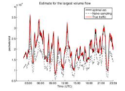
(a) Largest flow.

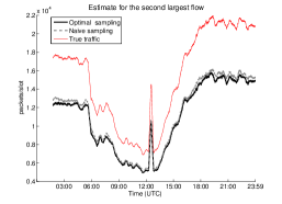
(b) Second largest flow.

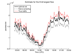
(c) Third largest flow.

Figure 3: Traffic estimation for different flows.

We use a real-world network, namely Internet2, to evaluate our algorithm. We juxtapose our method against a naïve sampling scheme (i.e., sampling rates not chosen optimally; Kalman filtering is still used though). Internet2 involves $L=26$ links, $N=9$ nodes and $J=72$ routes (see [28, 16]). In particular, we employ a dataset for traffic captured on March 17, 2009. The dataset includes the traffic volume of the $72$ flows, and the routing matrix $R$ (see Eq. (1)) which gives the path that each flow traverses in the network. In all examples that follow, a training window of $500$ time slots was applied to calibrate our model (see Step 1 of Algorithm 1).

In the naïve sampling scheme we evenly split the available sampling capacity among the competing flows of a link. We assume that the sampling capacity for each of the $26$ network links is $0.20$. Figure 2 shows the empirical root mean squared error (RMSE) for the whole network on the day of interest. RMSE is defined as, $RMSE(t)=\sqrt{\sum_{j\in\mathcal{J}}(\hat{x}_{j}(t|t)-x_{j}(t))^{2}/|J|}.$ The RMSE time average for the optimal sampling scheme is $1548$ packets per time slot, and $1773$ packets per time slot for the naïve one. This corresponds to a $13\%$ error reduction.

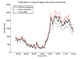
Figure 4: Long flow (4 hops), low volume.

We also examine traffic estimation for individual flows. Figures 3(a) – 3(c) present the cases for the three largest flows in terms of average traffic volume size, namely flows $19$, $66$ and $30$. Moreover, Figure 4 illustrates the estimation outcome for flow $14$, which is a “long” flow traversing $4$ links, but with relatively low traffic volume. Similarly, Figure 5, depicts the results for flow $68$, a “short” flow with low traffic volume. Clearly, the proposed approached is advantageous over the simplistic sampling scheme.

The results indicate the performance gains of our sampling scheme, being a result of considering both temporal and spatial correlation between flows. A necessary requirement, though, is the stationarity of traffic volumes. This does not always hold for Internet traffic. Ongoing work includes investigation of “richer” stochastic models, something that would allow sampling designs with even stricter sampling constraints (e.g., $1:100$ or even $1:1000$). Furthermore, one can additionally re-calibrate the model and “learn” its new parameters by increasing the frequency of the training periods (step 1 of Algorithm 1).

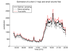
Figure 5: Short flow (1 hop), low volume.

References

- [1] D. P. Bertsekas and J. N. Tsitsiklis. Neuro Dynamic Programming. Athena Scientific, 1996.
- [2] S. Boyd and L. Vandenberghe. Convex Optimization. Cambridge University Press, 2004.
- [3] P. J. Brockwell and R. A. Davis. Time series: theory and methods. Springer-Verlag New York, Inc., New York, NY, USA, 1986.
- [4] D. Chua, E. Kolaczyk, and M. Crovella. Network kriging. Selected Areas in Communications, IEEE Journal on, 24(12):2263 –2272, dec. 2006.
- [5] K. C. Claffy, G. C. Polyzos, and H.-W. Braun. Application of sampling methodologies to network traffic characterization. SIGCOMM Comput. Commun. Rev., 23(4):194–203, Oct. 1993.
- [6] M. Coates, Y. Pointurier, and M. Rabbat. Compressed network monitoring for IP and all-optical networks. In Proc. 7th ACM SIGCOMM, pages 241–252. ACM, 2007.
- [7] E. Cohen, G. Cormode, and N. Duffield. Don’t let the negatives bring you down: sampling from streams of signed updates. In SIGMETRICS ’12, pages 343–354, New York, NY, USA, 2012. ACM.
- [8] E. Cohen, N. Duffield, H. Kaplan, C. Lund, and M. Thorup. Algorithms and estimators for accurate summarization of internet traffic. In IMC 2007, pages 265–278, NY, 2007. ACM.
- [9] N. Duffield. Fair sampling across network flow measurements. SIGMETRICS Perform. Eval. Rev., 40(1):367–378, June 2012.
- [10] N. Duffield, C. Lund, and M. Thorup. Properties and prediction of flow statistics from sampled packet streams. In In Proc. ACM SIGCOMM Internet Measurement, pages 159–171, 2002.
- [11] N. Duffield, C. Lund, and M. Thorup. Flow sampling under hard resource constraints. In SIGMETRICS 2004, pages 85–96, NY, 2004.
- [12] N. Duffield, C. Lund, and M. Thorup. Estimating flow distributions from sampled flow statistics. IEEE/ACM Trans. Net., 13(5):933–946, Oct. ’05.
- [13] N. Duffield, C. Lund, and M. Thorup. Learn more, sample less: control of volume and variance in network measurement. Information Theory, IEEE Trans, on, 51(5):1756 – 1775, may 2005.
- [14] N. Duffield, C. Lund, and M. Thorup. Optimal combination of sampled network measurements. In IMC 2005, pages 8–8, Berkeley, CA, USA, 2005. USENIX Association.
- [15] R. Horst, P. M. Pardalos, and N. V. Thoai. Introduction to Global Optimization. Kluwer Academic Publishers, The Netherlands, 1995.
- [16] Internet2. http://www.internet2.edu/observatory/.
- [17] R. E. Kalman. A New Approach to Linear Filtering and Prediction Problems. Transactions of the ASME, Journal of Basic Engineering, (82 (Series D)):35–45, 1960.
- [18] P. R. Kumar and P. Varaiya. Stochastic systems: estimation, identification and adaptive control. Prentice-Hall, Inc., NJ, USA, 1986.
- [19] A. Lakhina, M. Crovella, and C. Diot. Diagnosing network-wide traffic anomalies. SIGCOMM Comp. Comm. Rev., 34:219–230, Aug. 2004.
- [20] M. Lee, N. Duffield, and R. Kompella. Opportunistic flow-level latency estimation using consistent netflow. Networking, IEEE/ACM Transactions on, 20(1):139 –152, feb. 2012.
- [21] A. Medina, N. Taft, K. Salamatian, S. Bhattacharyya, and C. Diot. Traffic matrix estimation: existing techniques and new directions. In SIGCOMM ’02, pages 161–174, NY, 2002.
- [22] I. Meier, L., J. Peschon, and R. Dressler. Optimal control of measurement subsystems. Automatic Control, IEEE Trans. on, 12(5):528 –536, Oct ’67.
- [23] K. Papagiannaki, N. Taft, and A. Lakhina. A distributed approach to measure ip traffic matrices. In IMC 2004, pages 161–174, NY, 2004.
- [24] W. B. Powell. Approximate Dynamic Programming. John Wiley and Sons, Inc., 2007.
- [25] H. Robbins. Some Aspects of the Sequential Design of Experiments. Bulletin of the American Mathematical Society, 58(5):527–535, Sept. 1952.
- [26] H. Singhal and G. Michailidis. Optimal sampling in state space models with applications to network monitoring. In Proceedings of the 2008 ACM SIGMETRICS, pages 145–156, 2008.
- [27] A. Soule, A. Lakhina, N. Taft, K. Papagiannaki, K. Salamatian, A. Nucci, M. Crovella, and C. Diot. Traffic matrices: balancing measurements, inference and modeling. In 2005 ACM SIGMETRICS, pages 362–373, New York, NY, USA, 2005. ACM.
- [28] S. Stoev, G. Michailidis, and J. Vaughan. On global modeling of network traffic. Technical report, University of Michigan, 2010. http://www.stat.lsa.umich.edu/sstoev/global_tr.pdf.
- [29] N. V. Thoai and H. Tuy. Convergent algorithms for minimizing a concave function. Mathematics of Operations Research, 5(4):pp. 556–566, 1980.
- [30] H. Witsenhausen. Separation of estimation and control for discrete time systems. Proceedings of the IEEE, 59(11):1557 – 1566, nov. 1971.
- [31] L. Yang and G. Michailidis. Sampled based estimation of network traffic flow characteristics. In INFOCOM ’07., pages 1775 –1783, May 2007.
- [32] Y. Zhang, M. Roughan, C. Lund, and D. Donoho. An information-theoretic approach to traffic matrix estimation. In SIGCOMM 2003, pages 301–312, New York, NY, USA, 2003. ACM.