Spinon confinement: dynamics of weakly coupled Hubbard chains

Abstract

Using large-scale determinant quantum Monte Carlo simulations in combination with the stochastic analytical continuation, we study two-particle dynamical correlation functions in the anisotropic square lattice of weakly coupled one-dimensional (1D) Hubbard chains at half-filling and in the presence of weak frustration. The evolution of the static spin structure factor upon increasing the interchain coupling is suggestive of the transition from the power-law decay of spin-spin correlations in the 1D limit to long-range antiferromagnetic order in the quasi-1D regime and at $T=0$. In the numerically accessible regime of interchain couplings, the charge sector remains gapped. The low-energy momentum dependence of the spin excitations is well described by the linear spin-wave theory with the largest intensity located around the antiferromagnetic wave vector. This magnon mode corresponds to a bound state of two spinons. At higher energies the spinons deconfine and we observe signatures of the two-spinon continuum which progressively fade away as a function of interchain hopping.

I Introduction

In the realm of the solid state, controlling dimensionality implies that the thermal energy (or frequency) is larger that the effective coupling which triggers a dimensional crossover. Kivelson00 Under those circumstances, there is no coherence between the lower-dimensional units such that they effectively decouple. The dimensional crossover is particularly interesting when elementary excitations fractionalize in the lower-dimensional limit. Giamarchi_book For example, neutron scattering experiments on weakly coupled spin ladders of CaCu₂O₃ show the two-spinon continuum at frequencies larger than the interchain exchange and their confinement in the higher-dimensional ladder system emerging at lower energies. Lake10 Another experimental realization is provided by BaCu₂Si₂O₇ and KCuF₃ which consist of weakly coupled spin-1/2 chains. Zhe00 ; Zhe01 ; Lake05 At high frequencies one observes the two-spinon continuum, signalizing free spinons. In the low-frequency limit, pairs of spinons bind to form the Goldstone mode (spin-waves) of the broken-symmetry phase.

In addition to gapless transverse spin-wave excitations, nearly disordered by quantum fluctuations quasi-1D antiferromagnets are expected to exhibit anomalous (i.e., beyond the standard spin-wave theory) longitudinal mode at finite energy corresponding to fluctuations in the staggered magnetic moment. The presence of longitudinal spin excitations near the disordered transition has been predicted within the quantum Sine-Gordon field theory for weakly coupled to form an anisotropic cubic lattice spin-1/2 chains treating the interchain couplings as perturbation. Schultz96 ; Essler97 The longitudinal mode has been resolved in KCuF₃, Lake00 ; Lake05prb while so far only a broad continuum feature has been found in BaCu₂Si₂O₇. Zhe02 ; Zhe03

The dimensional crossover is not limited to spin systems but also plays the essential role in our understanding of Bechgaard salts. In these organic compounds a dimensional-crossover-driven insulator to metal Mott transition has been observed. Vescoli98 A complete theoretical description of this phenomenon is still missing and continues to capture interest. Bier01 ; Ess02 ; Tsu07 ; Rib11 ; Mou11 ; Raczkowski12

The aim of this paper is to study numerically the change in the nature of low-energy excitations on coupling one-dimensional (1D) half-filled Hubbard chains. In contrast to previous work, Raczkowski12 our aim is to study two-particle quantities: spin and charge dynamical structure factors. Since the 1D regime is dominated by strong momentum dependence of the self-energy, an accurate evaluation of the two-particle spectra requires the necessity to include vertex corrections. Hence, one faces a challenging task going beyond the dynamical cluster approximation schemes. Maier05 ; Kot06

To handle the full complexity of the problem, we have adopted the finite-temperature auxiliary-field quantum Monte Carlo (QMC) algorithm. BSS It allows us to carry out simulations on lattice sizes ranging up to $20\times 20$ in the presence of weak frustration and close to the 1D limit. Here, the limiting factor is the onset of the negative sign problem which ultimately leads to an exponential scaling of the computational time as a function of system size and inverse temperature $\beta=1/T$. We restrict our studies to the spin rotationally symmetric case and address the emergence of transverse spin-wave mode in a dimensional crossover from 1D to quasi-two-dimensional (2D) systems.

Our main results can be summarized as follows. 1D half-filled Hubbard chains are insulating due to the relevance of umklapp scattering. Below the charge gap, spin dynamics is characterized by the two-spinon continuum and absence of long-range magnetic order. Within our resolution, we shall see that this state is unstable towards interchain hopping, since down to our smallest considered values, the ground state develops long-range antiferromagnetic (AF) order. This result is consistent with the one put forward in Ref. Affleck94, and confirmed numerically in Refs. Sandvik99, ; Kim00, albeit in the absence of frustration and in the realm of quantum spin systems. This implies that for any value of interchain hopping, there is an energy scale Sandvik11 below which one will observe a crossover in the dynamical spin structure factor from a two-spinon continuum to a spin-wave mode. Our real-frequency QMC data, extracted by carrying out the stochastic analytic continuation Beach04a of the imaginary time-dependent spin-spin correlation function, provide ample support for this interpretation. In addition, our results indicate strong thermal effects in quantum magnets with weakly confined spinons. Vojta09

The paper is organized as follows. Section II defines the model Hamiltonians. Section III briefly describes approximate dynamical response of the spin system in two limiting cases: (i) the two-spinon continuum typical of the 1D spin chain can be accounted for within a SU(2) spin symmetric mean-field approximation, and (ii) spin dynamics of the 2D magnetically ordered phase at $T=0$ is conveniently described within the spin-wave theory. Anderson52 ; Kubo52 Section IV presents our main results, i.e, the dimensional-crossover-driven evolution of static as well as dynamical properties of the ground state. The conclusions are summarized in Sec. V.

II Models

We study the Hubbard model on a strongly anisotropic square lattice at half-filling,

$$H=-\sum_{\boldsymbol{ij},\sigma}t_{\boldsymbol{ij}}c^{{\dagger}}_{{\boldsymbol{i}}\sigma}c_{{\boldsymbol{j}}\sigma}+U\sum_{\boldsymbol{i}}n_{{\boldsymbol{i}}\uparrow}n_{{\boldsymbol{i}}\downarrow}-\mu\sum_{\boldsymbol{i},\sigma}n_{{\boldsymbol{i}}\sigma},$$ (1)

where the electron hopping $t_{\boldsymbol{ij}}$ is $t$ ($t_{\perp}$) on the intrachain (interchain) bonds, $\mu$ is the chemical potential and we set $U/t=3$. Due to perfect nesting of the Fermi surface, the Hubbard model (1) is expected to develop Néel order in the presence of any infinitesimally small interchain coupling in the $T=0$ limit. Affleck94 ; Sandvik99 ; Kim00 Here, we allow for a finite diagonal next-nearest neighbor hopping $t^{\prime}=-t_{\perp}/4$. It reduces nesting and makes the scenario of immediate magnetic ordering less obvious. Affleck96

Additionally, we consider the spin $S=1/2$ Heisenberg model with nearest neighbor interactions $J$ ($J_{\perp}$) along the intrachain (interchain) bonds, respectively, extended by next-nearest neighbor interaction $J^{\prime}$:

$$H_{J}=J\sum_{\langle\boldsymbol{ij}\rangle_{\parallel}}{\boldsymbol{S}}_{\boldsymbol{i}}\cdot{\boldsymbol{S}}_{\boldsymbol{j}}+J_{\perp}\sum_{\langle\boldsymbol{ij}\rangle_{\perp}}{\boldsymbol{S}}_{\boldsymbol{i}}\cdot{\boldsymbol{S}}_{\boldsymbol{j}}+J^{\prime}\sum_{\langle\langle\boldsymbol{ij}\rangle\rangle}{\boldsymbol{S}}_{\boldsymbol{i}}\cdot{\boldsymbol{S}}_{\boldsymbol{j}}.$$ (2)

The interaction $J^{\prime}$ competes with the tendency toward long-range AF order and gives rise to geometric frustration. We shall discuss in Sec. IV.2 to what extent spin-wave dispersion in the Heisenberg model describes the low-energy QMC spin excitations of the Hubbard model.

III Approximate spin dynamics

In this Section, we discuss two limiting cases of the spin dynamics: (i) two-spinon continuum typical in one-dimension, and (ii) spin-wave modes characteristic of a higher-dimensional magnetically ordered phase. The overall spectral features of the two limits can be reproduced using simple but different approximation schemes.

III.1 Two-spinon continuum in one-dimension

In the presence of any finite Hubbard interaction, the relevance of umklapp scattering in the 1D regime and at half-filling, opens a gap for charge excitations while leaving the spin sector gapless. Below the charge gap, one can model the relevant physics by a spin-only $S=1/2$ Heisenberg chain. In the 1D limit, the magnon excitation which one produces by flipping a spin decomposes into two spinons corresponding to domains walls in the AF background. Hence, the spin dynamics is characterized by the two-spinon continuum.

A simple understanding of this phenomenon is provided by a mean-field (MF) decoupling which conserves the SU(2) spin symmetry. Affleck88 Starting from the 1D Heisenberg model, one can adopt a fermion representation of the spin-operator ${\boldsymbol{S}}_{\boldsymbol{i}}=\frac{1}{2}\sum_{\sigma,\sigma^{\prime}}f^{\dagger}_{{\boldsymbol{i}},\sigma}\vec{\sigma}_{\sigma,\sigma^{\prime}}f_{{\boldsymbol{i}},\sigma^{\prime}}$ subject to the constraint,

$$\sum_{\sigma}f^{\dagger}_{{\boldsymbol{i}}\sigma}f_{{\boldsymbol{i}}\sigma}=1.$$ (3)

Next, using the relation:

$${\boldsymbol{S}}_{\boldsymbol{i}}\cdot{\boldsymbol{S}}_{\boldsymbol{j}}-\frac{1}{4}=-\frac{1}{4}\bigl{(}D^{\dagger}_{\boldsymbol{i}\boldsymbol{j}}D_{\boldsymbol{i}\boldsymbol{j}}+D_{\boldsymbol{i}\boldsymbol{j}}D^{\dagger}_{\boldsymbol{i}\boldsymbol{j}}\bigr{)},$$ (4)

with $D_{\boldsymbol{i}\boldsymbol{j}}=\sum_{\sigma}f^{\dagger}_{{\boldsymbol{i}},\sigma}f_{{\boldsymbol{j}},\sigma}$ and introducing the bond-order parameter $\chi=\langle D_{\boldsymbol{i}\boldsymbol{j}}\rangle$ yields the following MF Hamiltonian,

$$H^{\rm{MF}}_{\widetilde{J}}=-\widetilde{J}\sum_{\langle{\boldsymbol{i}}{\boldsymbol{j}}\rangle_{\parallel},\sigma}\bigl{(}f^{\dagger}_{{\boldsymbol{i}},\sigma}f_{{\boldsymbol{j}},\sigma}+f^{\dagger}_{{\boldsymbol{j}},\sigma}f_{{\boldsymbol{i}},\sigma}\bigr{)},$$ (5)

with a renormalized coupling $\widetilde{J}\equiv J\chi/2$. At the MF level, the constraint Eq. (3) is satisfied only on average, i.e., $\sum_{\sigma}\langle f^{\dagger}_{{\boldsymbol{i}},\sigma}f_{{\boldsymbol{i}},\sigma}\rangle=1$, such that the spinon Fermi wave vector reads $k_{\rm F}=\pi/2$. Finally, the corresponding spin susceptibility in the $z$-direction is given by,

$$\chi_{s}(\boldsymbol{q},\omega)=\frac{1}{4N}\sum_{{\boldsymbol{k}}}\frac{f_{\rm F}(\boldsymbol{k}+\boldsymbol{q})-f_{\rm F}(\boldsymbol{k})}{\varepsilon({\boldsymbol{k})}-\varepsilon({\boldsymbol{k}+\boldsymbol{q})-\omega-i\delta}},$$ (6)

where $f_{\rm F}(\boldsymbol{k})$ is the Fermi function and $\varepsilon({\boldsymbol{k})}$ is the 1D tight-binding dispersion of the MF Hamiltonian Eq. (5). The intensity plot of $\chi_{s}(\boldsymbol{q},\omega)$ is shown in Fig. 1. It depicts the two-spinon continuum with two gapless excitations at ${\boldsymbol{q}}=0$ and ${\boldsymbol{q}}=2k_{\rm F}=\pi$.

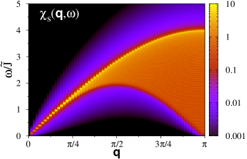
Figure 1: (Color online) Two-spinon continuum of the spin susceptibility $\chi_{s}(\boldsymbol{q},\omega)$ Eq. (6) as obtained from the SU(2) spin symmetric MF approximation of the 1D Heisenberg model.

III.2 Linear spin-wave theory

In spatial dimensions greater than one, the spinons bind and form magnons, which are nothing but the Goldstone modes of the continuous SU(2) spin broken symmetry. The magnons are well accounted within the linear spin-wave theory (LSWT) in the leading $1/S$ order. Anderson52 ; Kubo52 The spin-wave expansion is valid about the ground state with a finite classical order parameter. In contrast, there is no long-range order in one-dimension and the magnons decay into pairs of spinons. The signature of spin fractalization is then seen as continuum of excited states. Clearly, the dimensional crossover must affect the nature of elementary spin excitations. In particular, when spinons bind, the continuum of excitations in the dynamical spin structure factor is expected to give way to well defined sharp magnon peaks described by the LSWT.

Below we discuss the LSWT magnon dispersion as well as quantum corrections to the magnetic order parameter $\langle S^{z}\rangle$. We focus on the AF phase within the anisotropic Heisenberg model defined in Eq. (2). The starting point is the Holstein-Primakoff transformation expressing the spin operators in terms of bosonic operators $\{a_{i}^{\dagger},a_{i}\}$,

$$S_{i}^{z}=S-a_{i}^{\dagger}a_{i},\hskip 14.22636ptS_{i}^{+}\simeq\sqrt{2S}a_{i},\hskip 14.22636ptS_{i}^{-}\simeq\sqrt{2S}a_{i}^{\dagger}.$$ (7)

The effective bosonic problem is then solved by employing subsequent Fourier and Bogoliubov transformations. The latter diagonalizes a $2\times 2$ dynamical matrix at each momentum q. The corresponding magnon dispersion reads,

$$\omega_{\boldsymbol{q}}=2S\sqrt{\xi^{2}_{\boldsymbol{q}}-\gamma^{2}_{\boldsymbol{q}}},$$ (8)

with 2D structure factors,

$$\xi_{\boldsymbol{q}} =J+J_{\perp}-2J^{\prime}(1-\cos q_{x}\cos q_{y}),$$ (9)

$$\gamma_{\boldsymbol{q}} =J\cos q_{x}+J_{\perp}\cos q_{y}.$$ (10)

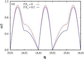
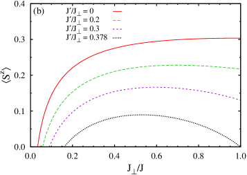
Figure 2: (Color online) (a) Spin-wave dispersion in the AF phase within the anisotropic $S=1/2$ Heisenberg model (2) with $J_{\perp}/J=0.1$; (b) Effective magnetic order parameter Eq. (13) within the LSWT as a function of increasing interchain interaction $J_{\perp}$.

Spin-wave dispersion of the Heisenberg model (2) with $J^{\prime}=0$ is displayed for a representative value of $J_{\perp}/J=0.1$ in Fig. 2(a). The low-energy part of the spectrum is given by gapless Goldstone modes with a linear momentum dependence,

$$\omega_{\alpha}({\boldsymbol{q}})\simeq D_{\alpha}{{\boldsymbol{q}}},$$ (11)

with $D_{\parallel}$ ($D_{\perp}$) being the spin-wave stiffness along (perpendicular to) the chains, respectively. We compare it with the dispersion obtained with a finite frustrated interaction $J^{\prime}$. One observes in Fig. 2(a) that even small $J^{\prime}/J_{\perp}=0.2$ modifies the magnon dispersion. In particular, the frustration manifests itself as: (i) flattening of the magnon band around momenta ${\boldsymbol{q}}=(\pi,0)$ and ${\boldsymbol{q}}=(0,\pi)$, and (ii) reduction of the stiffness constant $D_{\perp}$ leaving $D_{\parallel}$ almost intact.

It is instructive to consider the effect of quantum fluctuations on the classical order parameter $S$ in the presence of frustrated interaction $J^{\prime}$. Using the standard scheme of the LSWT, Raczkowski02 one can show that the size of quantum corrections in the $T\to 0$ limit is given by,

$$\delta\langle S^{z}\rangle=S\int\frac{d^{2}{\boldsymbol{q}}}{(2\pi)^{2}}\frac{\xi_{\boldsymbol{q}}}{\omega_{\boldsymbol{q}}}-\frac{1}{2}.$$ (12)

The effective magnetic order parameter,

$$\langle S^{z}\rangle=S-\delta\langle S^{z}\rangle,$$ (13)

for spin $S=1/2$ is plotted as a function of $J_{\perp}$ in Fig. 2(b). On the one hand, previous QMC studies of weakly coupled $S=1/2$ Heisenberg chains, Sandvik99 ; Kim00 reveal that a finite critical value $J_{\perp}^{*}/J\simeq 0.03$ required for the onset of long-range AF order is an artifact of the LSWT. The failure follows from the increased importance of higher-order corrections to the local order parameter $\langle S^{z}\rangle$ in the 1D limit. Iga05 On the other hand, the LSWT captures the frustrating role of next-nearest neighbor coupling $J^{\prime}$ and predicts noticeable enhancement of $J_{\perp}^{*}$. We list critical $J_{\perp}^{*}$ for a few representative values of $J^{\prime}$ in Table 1. Among them, $J^{\prime}/J_{\perp}=0.378$ is expected within the LSWT to fully suppress long-range AF order in the isotropic 2D limit. The same tendency has been found in the QMC simulations of the half-filled 2D Hubbard model when the next-nearest neighbor hopping is sufficiently large. Hirsch87

Table 1: Critical value $J_{\perp}^{*}$ required to stabilize long-range AF order in the quasi-1D regime in the presence of frustrated coupling $J^{\prime}$.

$J^{\prime}/J_{\perp}$		0		0.2		0.3		0.378
$J_{\perp}^{*}/J$		0.033		0.058		0.09		0.162

IV Results

We proceed now to present our QMC results for the Hubbard model (1). The results were obtained using a finite-temperature implementation of the auxiliary-field QMC algorithm (see Ref. Assaad08_rev, and references therein). It involves a separation of the one-body kinetic $H_{t}$ and two-body Hubbard interaction $H_{U}$ terms with the help of the Trotter decomposition,

$$e^{-\Delta\tau\left(H_{U}+H_{t}\right)}\simeq e^{-\Delta\tau H_{U}}e^{-\Delta\tau H_{t}}.$$ (14)

Typically, we have used a finite imaginary time step $\Delta\tau t=1/6$. This introduces an overall controlled systematic error of order $(\Delta\tau)^{2}$. Finally, we have opted for a discrete, Ising, Hubbard-Stratonovitch field coupling to the $z$-component of the magnetization. With this setup, we have carried out simulations for lattice sizes ranging from $L=8$ to $L=20$ and in the broad range of temperatures $t/5\leq T\leq t/30$. Severe minus-sign problem arising due to a finite next-nearest neighbor hopping $t^{\prime}=-t_{\perp}/4$ disabled QMC simulations beyond $t_{\perp}/t=0.35$.

IV.1 Equal time spin-spin correlation

A salient feature of the 1D interacting system is the power-law decay of all correlation functions. Giamarchi_book To investigate dimensional-crossover-driven effects in the nature of spin degrees of freedom, we calculate Fourier transform of the equal-time spin-spin correlations,

$$S({\boldsymbol{q}})=\frac{4}{3}\sum_{{\boldsymbol{r}}}e^{i{\boldsymbol{q}}\cdot{\boldsymbol{r}}}\langle{\boldsymbol{S}}({\boldsymbol{r}})\cdot{\boldsymbol{S}}({\boldsymbol{0}})\rangle.$$ (15)

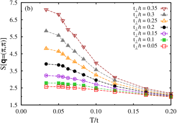
Figure 3: (Color online) Temperature dependence of the static spin structure factor $S({\boldsymbol{q}})$ found on the 16$\times 16$ lattice at momentum: (a) ${\boldsymbol{q}}=(\pi,0)$ and (b) ${\boldsymbol{q}}=(\pi,\pi)$.

Figure 3(a) illustrates temperature dependence of the static spin structure factor $S(\pi,0)$. This observable measures spin-spin correlations along the chains. One finds that the low-$T$ enhancement of $S(\pi,0)$ in the 1D limit is progressively replaced by a flat behavior on increasing $t_{\perp}$. The observed change is consistent with a transition from the power-law decay of spin-spin correlations in the isolated chains to an exponential falloff in the system of weakly coupled chains. However, sufficiently high temperature, i.e., larger than warping of the Fermi surface, should restore the 1D behavior of the spin-spin correlations. This indeed happens close to $T=t/5$ since the value of the spin structure factor $S(\pi,0)$ for $t_{\perp}/t=0.05$ almost matches that of the 1D regime, see Fig. 3(a).

The low-$T$ increase of staggered spin structure factor $S(\pi,\pi)$ shown in Fig. 3(b), is suggestive of the transition triggered by $t_{\perp}$ to the AF phase. To provide further support for the onset of broken-symmetry ground state, we plot in Fig. 4 finite-size scaling of the staggered magnetic moment,

$$m_{s}=\lim_{L\to\infty}\sqrt{\frac{S(\pi,\pi)}{L^{2}}}.$$ (16)

Down to our smallest considered values $t_{\perp}/t=0.05$ and in the effective zero-temperature limit, a finite value of $m_{s}$ is found in the thermodynamic limit. Clearly, the weak frustration brought by small $t^{\prime}=-t_{\perp}/4$ does not prevent the formation of long-range AF order. The absence of finite critical interchain coupling is supported by neutron scattering data on Sr₂CuO₃, a quasi-1D $S=1/2$ antiferromagnet with a very small Néel temperature $T_{N}/J\simeq 5K$. In this case a continuous reduction of the magnetic moment in the limit of vanishing interchain interactions has been found. Shirane97

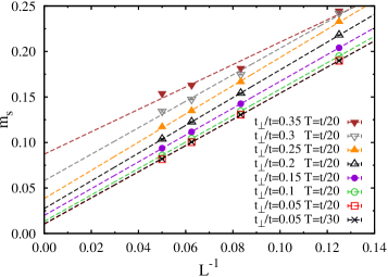
Figure 4: (Color online) Finite size extrapolation of the staggered magnetic moment $m_{s}$.

IV.2 Spin and charge dynamics

Having found the signatures of long-range AF order in the static spin-spin correlation function $S(\pi,\pi)$, we proceed to discuss spin $S({\boldsymbol{q}},\omega)$ and charge $C({\boldsymbol{q}},\omega)$ dynamical structure factors defined as:

$$S({\boldsymbol{q}},\omega)=\frac{\chi_{s}^{\prime\prime}({\boldsymbol{q}},\omega)}{1-e^{-\beta\omega}}\;\;{\rm and}\;\;C({\boldsymbol{q}},\omega)=\frac{\chi_{c}^{\prime\prime}({\boldsymbol{q}},\omega)}{1-e^{-\beta\omega}}.$$ (17)

Here, $\chi_{c}$ and $\chi_{s}$ correspond to the generalized charge and spin susceptibilities. The susceptibilities can be obtained from imaginary-time displaced two-particle correlation functions,

$$\langle S^{z}({\boldsymbol{q}},\tau)S^{z}(-{\boldsymbol{q}},0)\rangle =\frac{1}{\pi}\int{\rm d}w\;\frac{e^{-\omega\tau}}{1-e^{-\beta\omega}}\;\chi_{s}^{\prime\prime}({\boldsymbol{q}},\omega),$$ (18)

$$\langle N({\boldsymbol{q}},\tau)N(-{\boldsymbol{q}},0)\rangle =\frac{1}{\pi}\int{\rm d}w\;\frac{e^{-\omega\tau}}{1-e^{-\beta\omega}}\;\chi_{c}^{\prime\prime}({\boldsymbol{q}},\omega),$$ (19)

where,

$$S^{z}({\boldsymbol{q}}) =\frac{1}{\sqrt{L}}\sum_{\boldsymbol{r}}e^{i{\boldsymbol{q}}\cdot{\boldsymbol{r}}}\left(n_{{\boldsymbol{r}}\uparrow}-n_{{\boldsymbol{r}}\downarrow}\right),$$ (20)

$$N({\boldsymbol{q}}) =\frac{1}{\sqrt{L}}\sum_{\boldsymbol{r}}e^{i{\boldsymbol{q}}\cdot{\boldsymbol{r}}}\left(n_{{\boldsymbol{r}}\uparrow}+n_{{\boldsymbol{r}}\downarrow}-n\right).$$ (21)

with $n=\sum_{\sigma}\langle n_{{\boldsymbol{r}},\sigma}\rangle$ being the average filling level. We extracted the real-frequency two-particle spectra by analytically continuing the imaginary-time QMC data with the use of a stochastic version of the Maximum Entropy method. Beach04a

The dynamical spin structure factor $S({\boldsymbol{q}},\omega)$ is related to the static one $S({\boldsymbol{q}})$ through the sum rule:

$$S({\boldsymbol{q}})=\frac{1}{\pi}\int{\rm d}w\;S({\boldsymbol{q}},\omega).$$ (22)

Hence, we shall resolve in $S({\boldsymbol{q}},\omega)$ redistribution of magnetic spectral weight in the thermally-driven dimensional crossover. The latter was anticipated in Sec. IV.1 from the evolution of the static spin-spin correlation function $S({\boldsymbol{q}})$, see Fig. 3. However, our primary goal is to elucidate the evolution of the two-spinon continuum typical of the $S=1/2$ Heisenberg chain into the single-magnon mode known as a low-energy magnetic excitation in a 2D antiferromagnetically ordered phase at $T=0$. Jarrell92 ; Sandvik01 ; Scalettar02

IV.2.1 1D limit: deconfined spinons

We begin with the system of isolated ($t_{\perp}=0$) half-filled 1D Hubbard chains. The corresponding intensity plots of the spin and charge excitation spectrum are shown in Figs. 5 and 6. In the realm of bosonization, spin and charge degrees of freedom decouple. The energy scale, as measured from the Fermi energy, up to which this picture survives depends on the strength of the interaction. For example, in the single-particle spectra signatures of spin-charge separation are detected up to very high energies for interactions of the order of the bandwidth. Abend06 Beyond this energy scale, one would expect to recover the noninteracting picture where the spin and charge dynamical structure factors have equivalent supports. This regime corresponds to the particle-hole continuum. With this in mind, we can analyze the data of Figs. 5 and 6. At first glance, one will not detect a particle-hole continuum – as defined above – within the plotted energy range indicative of dominant role of vertex corrections. Hence the data, again in the considered energy range, should be understood in terms of collective spin and charge excitations.

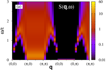
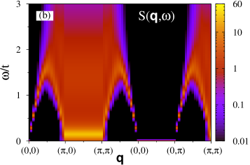
Figure 5: (Color online) Dynamical spin structure factor $S({\boldsymbol{q}},\omega)$ obtained on: (a) 16-site chain at $T=t/10$ and (b) 32-site chain at $T=t/20$.

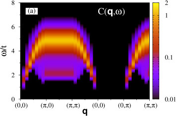
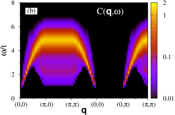
Figure 6: (Color online) Dynamical charge structure factor $C({\boldsymbol{q}},\omega)$ obtained on: (a) 16-site chain at $T=t/10$ and (b) 32-site chain at $T=t/20$.

The dynamic charge structure factor $C({\boldsymbol{q}},\omega)$ shows features similar to those seen in Ref. Penc12, using time-dependent density matrix renormalization group. The charge sector is gapped with a relatively large charge gap $\Delta/t>1$ (c.f. Fig. 6). Above the charge gap, one can detect aspects of the charge dynamics of Luttinger liquids, with low-lying charge excitations located at long wavelengths as well as at ${\boldsymbol{q}}=2k_{\rm F}=\pi$. Since the charge is fully gapped, the spin dynamics can be understood predominantly with a spin-only model which we will approximate by the $S=1/2$ Heisenberg chain. Its most prominent feature is the two-spinon continuum of states bounded from below and above by,  Clo62 ; Yam69

$$\frac{\pi}{2}J|\sin({\boldsymbol{q}})|\leq\omega({\boldsymbol{q}})\leq\pi J|\sin({\boldsymbol{q}}/2)|.$$ (23)

The upper bound corresponds to two spinons with the same momentum ${\boldsymbol{q}}/2$. The lowest-lying excited states come from two-spinons in which one spinon has momentum ${\boldsymbol{q}}$ and the other has zero or $\pi$. As shown in Fig. 5(b), these excitations carry the main spectral weight at low-$T$ as expected in the strong coupling regime $U/t\gg 1$ dominated by virtual hopping of electrons. Jarrell93 ; Sandvik97 ; Essler05 ; Ben07 ; Barthel09 This should be contrasted with the MF spectrum in Fig. 1. Although the latter reproduces the overall form of $S({\boldsymbol{q}},\omega)$, it is biased with respect to the distribution of weight since the MF approximation does not capture the criticality of the SU(2) spin-chain correctly. In this respect, the MF spectrum is similar to $S({\boldsymbol{q}},\omega)$ obtained in the weak coupling limit $U/t\ll 1$ with strong electron itinerancy effects. Essler05

The presence of zero-frequency magnetic weight at ${\boldsymbol{q}}=\pi$ and equivalent momenta shall give rise to immediate binding of spinons on coupling the 1D chains. This conjecture, supported by the analysis of the static spin structure factor $S(\pi,\pi)$ in Sec. IV.1, is suggestive of the emergence of low-energy spin-waves characteristic of the magnetically ordered phase. In contrast, no spectral weight in the charge and spin sector is found along the $(0,0)\to(0,\pi)$ direction, i.e., perpendicular to the chains. Hence, the dynamics of the dimensional crossover should be particularly clearly visible in this part of the Brillouin zone.

IV.2.2 Spinon confinement in the quasi-1D limit

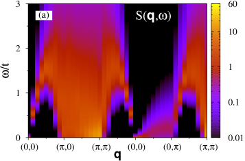
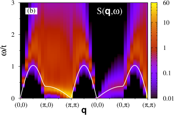
Figure 7: (Color online) Dynamical spin structure factor $S({\boldsymbol{q}},\omega)$ obtained on the $16\times 16$ lattice with $t_{\perp}/t=0.2$ at: (a) $T=t/10$ and (b) $T=t/20$. Solid line in the lower plot gives a LSWT fit Eq. (8) with $J_{\perp}/J=0.06$ and $J^{\prime}/J_{\perp}=0.2$.

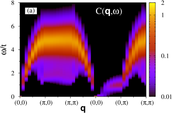
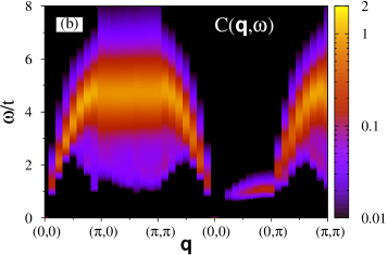
Figure 8: (Color online) Dynamical charge structure factor $C({\boldsymbol{q}},\omega)$ obtained on the $16\times 16$ lattice with $t_{\perp}/t=0.2$ at: (a) $T=t/10$ and (b) $T=t/20$.

We turn now to spin and charge excitation spectra of weakly coupled Hubbard chains. Coupling the chains affects first the low-frequency spin excitations. However, due to a small velocity, the spin-wave mode in the small regime of $t_{\perp}$ might be resolved only at sufficiently low-$T$. Hence, we begin the discussion by showing the data at $t_{\perp}/t=0.2$, and $T=t/10$, see Fig. 7(a). In this case one clearly observes: (i) reduction of $S({\boldsymbol{q}},\omega)$ around momentum ${\boldsymbol{q}}=(\pi,0)$ with respect to the 1D regime; (ii) buildup of the magnetic weight at the AF wave vector ${\boldsymbol{q}}=(\pi,\pi)$, and (iii) emergence of a broad incoherent feature along the $(0,0)\to(0,\pi)$ direction. Upon decreasing temperature down to $T=t/20$, the features (i) and (ii) evolve into a gapless spin-wave mode, see Fig. 7(b). It replaces the low-energy part of the two-spinon continuum. This should be contrasted with spinon confinement in a two-leg Hubbard Hur01 or spin $S=1/2$ Heisenberg Dagotto92 ; Shelton96 ; Greiter02a ; Greiter02b ladder systems with a finite interchain coupling leading to a singlet ground state with gapped magnons.

Spinon confinement is also reflected in the overall loss of spectral weight of the two-spinon continuum. This effect is particularly strong around the AF wave vector ${\boldsymbol{q}}=(\pi,\pi)$ where the low-energy magnetic intensity quickly fades away on moving to higher frequencies.

As shown in Fig. 7(b), the LSWT dispersion relation Eq. (8) provides quite a good description of the low-energy part of the magnon spectrum along the $(\pi,\pi)\to(\pi,0)$ path. However, a certain discrepancy emerges at higher energies. Note, that for the chosen fitting parameters $J_{\perp}/J=0.06$ and $J^{\prime}/J_{\perp}=0.2$, the LSWT yields a finite magnetic order parameter $\langle S^{z}\rangle$ (see Table 1) consistent with the long-range AF order in the system. Spectral weight is also found along the $(0,0)\to(0,\pi)$ direction. However, its intensity is low and vanishes in the $|{\boldsymbol{q}}|\to 0$ limit. Furthermore, there is a clear anisotropy in the spin-wave velocity. The small velocity associated with the interchain dispersion relation, i.e., from $(0,0)\to(0,\pi)$, renders thermal effects stronger, and could provide an explanation for the broad line shape even in the low-energy limit. On the other hand and at higher energies, the magnon can decay into spinons, thus providing a damping mechanism of the magnon mode.

The dimensional crossover is also seen in the charge dynamics shown in Fig. 8. Indeed, the comparison with the 1D case (see Fig. 6) reveals: (i) disappearance of the 1D 2$k_{\rm F}$ feature observed in Fig. 6, and (ii) emergence of a broad charge mode dispersing along the $(0,0)\to(0,\pi)$ direction. As depicted in Fig. 8(b), its low-frequency weight is washed out on decreasing temperature down to $T=t/20$. This is consistent with the localization of charges as appropriate for the insulating state.

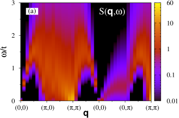
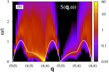
Figure 9: (Color online) Same as in Fig. 7 but for $t_{\perp}/t=0.3$. Solid line in the lower plot gives a LSWT fit Eq. (8) with $J_{\perp}/J=0.1$ and $J^{\prime}/J_{\perp}=0.2$.

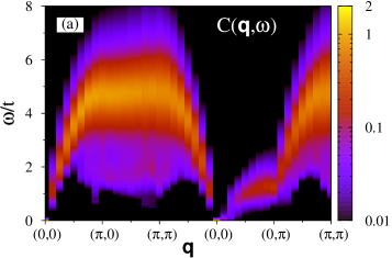
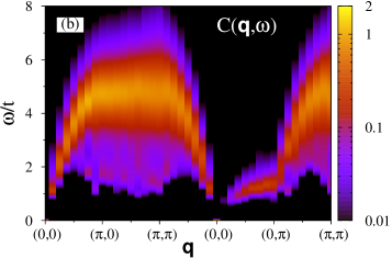
Figure 10: (Color online) Same as in Fig. 8 but for $t_{\perp}/t=0.3$.

The inspection of both the dynamical spin, $S({\boldsymbol{q}},\omega)$, and charge, $C({\boldsymbol{q}},\omega)$, structure factors allows us to identify essentially two frequency regimes dominated by magnetic excitations of different nature: (i) low-frequency magnons, and (ii) intermediate-frequency two-spinon excitations. We interpret this energy-scale separation as follows. Coupling the chains triggers binding of spinons into low-energy spin-waves. However, deconfinement of spinons still occurs above a threshold energy set up by the strength of attractive potential between the spinons. In proximity to the 1D regime, this potential might be easily overcome by thermal fluctuations. This accounts for the observed transfer magnetic weight out of the magnon peak into the two-spinon continuum. We illustrate this effect in Fig. 7 which compares $S({\boldsymbol{q}},\omega)$ for two different temperatures $T=t/10$ and $T=t/20$.

Let us now make a comparison between the spin excitation spectra $S({\boldsymbol{q}},\omega)$ found at $t_{\perp}/t=0.2$ and $t_{\perp}/t=0.3$. The latter is shown in Fig. 9. It may be seen that at low temperature $T=t/20$ the spin-wave mode acquires progressively increasing damping on going from $(\pi,\pi)$ to $(\pi,0)$, see Fig. 9(b). This should be contrasted with $S({\boldsymbol{q}},\omega)$ at $t_{\perp}/t=0.2$ where the magnon dispersion is clearly resolved across the whole $(\pi,\pi)\to(\pi,0)$ path, see Fig. 7(b). We ascribe this enhanced decay rate to larger bandwidth of the spin-wave dispersion. As a result, magnon excitations reach frequencies high-enough to couple with charge excitations. Hence, in contrast to $t_{\perp}/t=0.2$ with a single decay chanel, i.e., into pairs of spinons, spin-waves at $t_{\perp}/t=0.3$ might also spontaneously decay into charge excitations. Nevertheless, the low-energy part of the magnon dispersion is fairly well accounted within the LSWT, see Fig. 9(b).

Stronger spinon confinement expected for $t_{\perp}/t=0.3$ is consistent with larger amount of the magnon weight perpendicular to the chains, i.e., along the $(0,0)\to(0,\pi)$ path. Accumulation of spectral weight along the same $(0,0)\to(0,\pi)$ direction is also observed in the charge excitation spectrum $C({\boldsymbol{q}},\omega)$, see Fig. 10. It reflects development of charge correlations between the chains. In contrast, there are no zero-frequency charge excitations in the low-temperature regime $T=t/20$ typical of the insulating phase, see Fig. 10(b). However, this finite-energy charge mode might be considered as a precursor feature of electron deconfinement, i.e., possibility of the charge transfer across the chains in the dimensional-crossover-driven Mott transition. Raczkowski12 Finally, a weak momentum dependence of charge excitations may be resolved along the $(\pi,0)\to(\pi,\pi)$ path.

V Conclusions

We have systematically studied the evolution of spin and charge degrees of freedom upon coupling the 1D Hubbard chains with frustrating hopping matrix elements. From the technical point of view, we tackled the problem with the numerically exact finite-temperature auxiliary-field QMC algorithm on lattice sizes up to $20\times 20$. At the considered value of $U/t=3$ and up to $t_{\perp}/t=0.35$, the sign problem turned out to be manageable down to $T=t/20$. In this parameter regime, the low-temperature dynamical charge structure factor shows that the system remains insulating.

The 1D limit is very well understood. Giamarchi_book The relevance of umklapp processes at half-filling opens a charge gap and results in critical equal-time spin-spin correlations. The spin dynamical structure factor exhibits the two-spinon continuum with gapless excitations at long wavelengths and at ${\boldsymbol{q}}=\pi$. Upon coupling the chains, our results support the direct onset of a broken-symmetry AF ground state. This result implies that spinons will bind into magnons as soon as the chains are coupled.

Our numerical results for the dynamical spin structure factor resolve the frequency and temperature dependence of the transition from deconfined to confined spinons. In particular, a transverse spin-wave mode emerges in the low-energy sector of the dynamical spin structure factor. This spin-wave mode is heavily damped since it can decay into pair of spinons present at higher energies. The overall high-energy features of the dynamical spin structure factor show clear signatures of the two-spinon continuum which progressively fade away as the interchain coupling is enhanced. The same is valid for the dynamical charge structure factor which shows robust 1D features at energy scales beyond the charge gap and up to our largest value of the interchain coupling.

Finally, let us discuss a possible experimental relevance of our results. A similar crossover in the nature of spin excitations from dispersive scattering continua to sharp magnon modes at the lowest energies has been observed below the ordering temperature $T_{N}$ in a moderately anisotropic triangular lattice of a $S=1/2$ antiferromagnet Cs₂CuCl₄. Coldea01 ; Coldea03 The complex structure of magnetic excitations has been ascribed in this case to the proximity of Cs₂CuCl₄ to a fractionalized spin liquid phase which sets up as a result of an effective dimensional reduction by the strong geometric frustration. Kohno07

The coexistence of the one- and higher-dimensional transverse spin dynamics operating at different frequency scales, has also been resolved in the inelastic neutron scattering data on BaCu₂Si₂O₇ and KCuF₃, both of them consisting of weakly coupled $S=1/2$ chains. Zhe00 ; Zhe01 ; Lake05 A detailed comparison of the dynamical spin correlation function $S({\boldsymbol{q}},\omega)$ for the anisotropic $A$-type antiferromagnetic ($A$-AF) phase of KCuF₃ should take into account a weak ferromagnetic superexchange between the AF chains. The latter is expected to facilitate the formation of spin-waves by reducing quantum corrections to the order parameter in the $A$-AF phase. Raczkowski02 As such, it might shift a threshold energy above which one recovers the two-spinon continuum towards higher energies as compared to the antiferromagnet with solely AF interactions.

We conclude that the simultaneous observation of low-energy magnons and high-energy spinons is a fingerprint of magnetically ordered phase coexisting with strong quantum fluctuations brought by reduced dimensionality.

- (1) E. W. Carlson, D. Orgad, S. A. Kivelson, and V. J. Emery, Phys. Rev. B 62, 3422 (2000)
- (2) T. Giamarchi, Quantum Physics in One Dimension (Oxford University, Oxford, 2004)
- (3) B. Lake, A. M. Tsvelik, S. Notbohm, D. A. Tennant, T. G. Perring, M. Reehuis, C. Sekar, G. Krabbes, and B. Büchner, Nat. Phys. 6, 50 (2010)
- (4) A. Zheludev, M. Kenzelmann, S. Raymond, E. Ressouche, T. Masuda, K. Kakurai, S. Maslov, I. Tsukada, K. Uchinokura, and A. Wildes, Phys. Rev. Lett. 85, 4799 (2000)
- (5) M. Kenzelmann, A. Zheludev, S. Raymond, E. Ressouche, T. Masuda, P. Böni, K. Kakurai, I. Tsukada, K. Uchinokura, and R. Coldea, Phys. Rev. B 64, 054422 (2001)
- (6) B. Lake, D. A. Tennant, C. D. Frost, and S. E. Nagler, Nat. Mater. 4, 329 (2005)
- (7) H. J. Schulz, Phys. Rev. Lett. 77, 2790 (1996)
- (8) F. H. L. Essler, A. M. Tsvelik, and G. Delfino, Phys. Rev. B 56, 11001 (1997)
- (9) B. Lake, D. A. Tennant, and S. E. Nagler, Phys. Rev. Lett. 85, 832 (2000)
- (10) B. Lake, D. A. Tennant, and S. E. Nagler, Phys. Rev. B 71, 134412 (2005)
- (11) A. Zheludev, K. Kakurai, T. Masuda, K. Uchinokura, and K. Nakajima, Phys. Rev. Lett. 89, 197205 (2002)
- (12) A. Zheludev, S. Raymond, L.-P. Regnault, F. H. L. Essler, K. Kakurai, T. Masuda, and K. Uchinokura, Phys. Rev. B 67, 134406 (2003)
- (13) V. Vescoli, L. Degiorgi, W. Henderson, G. Grüner, K. Starkey, and L. K. Montgomery, Science 281, 1181 (1998)
- (14) S. Biermann, A. Georges, A. Lichtenstein, and T. Giamarchi, Phys. Rev. Lett. 87, 276405 (2001)
- (15) F. H. L. Essler and A. M. Tsvelik, Phys. Rev. B 65, 115117 (2002)
- (16) M. Tsuchiizu, Y. Suzumura, and C. Bourbonnais, Phys. Rev. Lett. 99, 126404 (2007)
- (17) P. Ribeiro, P. D. Sacramento, and K. Penc, Phys. Rev. B 84, 045112 (2011)
- (18) S. Moukouri and E. Eidelstein, Phys. Rev. B 84, 193103 (2011)
- (19) M. Raczkowski and F. F. Assaad, Phys. Rev. Lett. 109, 126404 (2012)
- (20) T. Maier, M. Jarrell, T. Pruschke, and M. H. Hettler, Rev. Mod. Phys. 77, 1027 (2005)
- (21) G. Kotliar, S. Y. Savrasov, K. Haule, V. S. Oudovenko, O. Parcollet, and C. A. Marianetti, Rev. Mod. Phys. 78, 865 (2006)
- (22) R. Blankenbecler, D. J. Scalapino, and R. L. Sugar, Phys. Rev. D 24, 2278 (1981)
- (23) I. Affleck, M. P. Gelfand, and R. R. P. Singh, J. Phys. A: Math. Gen. 27, 7313 (1994)
- (24) A. W. Sandvik, Phys. Rev. Lett. 83, 3069 (1999)
- (25) Y. J. Kim and R. J. Birgeneau, Phys. Rev. B 62, 6378 (2000)
- (26) Y. Tang and A. W. Sandvik, Phys. Rev. Lett. 107, 157201 (2011)
- (27) K. S. D. Beach, e-print arXiv:cond-mat/0403055 (2004)
- (28) R. L. Doretto and M. Vojta, Phys. Rev. B 80, 024411 (2009)
- (29) P. W. Anderson, Phys. Rev. 86, 694 (1952)
- (30) R. Kubo, Phys. Rev. 87, 568 (1952)
- (31) I. Affleck and B. I. Halperin, J. Phys. A: Math. Gen. 29, 2627 (1996)
- (32) I. Affleck and J. B. Marston, Phys. Rev. B 37, 3774 (1988)
- (33) M. Raczkowski and A. M. Oleś, Phys. Rev. B 66, 094431 (2002)
- (34) J. I. Igarashi and T. Nagao, Phys. Rev. B 72, 014403 (2005)
- (35) H. Q. Lin and J. E. Hirsch, Phys. Rev. B 35, 3359 (1987)
- (36) F. F. Assaad and H. G. Evertz, in Computational Many Particle Physics, Lecture Notes in Physics, Vol. 739, edited by H. Fehske, R. Schneider, and A. Weiße (Springer Verlag, Berlin, 2008) pp. 277–356
- (37) K. M. Kojima, Y. Fudamoto, M. Larkin, G. M. Luke, J. Merrin, B. Nachumi, Y. J. Uemura, N. Motoyama, H. Eisaki, S. Uchida, K. Yamada, Y. Endoh, S. Hosoya, B. J. Sternlieb, and G. Shirane, Phys. Rev. Lett. 78, 1787 (1997)
- (38) M. Makivić and M. Jarrell, Phys. Rev. Lett. 68, 1770 (1992)
- (39) A. W. Sandvik and R. R. P. Singh, Phys. Rev. Lett. 86, 528 (2001)
- (40) P. Sengupta, R. T. Scalettar, and R. R. P. Singh, Phys. Rev. B 66, 144420 (2002)
- (41) A. Abendschein and F. F. Assaad, Phys. Rev. B 73, 165119 (2006)
- (42) R. G. Pereira, K. Penc, S. R. White, P. D. Sacramento, and J. M. P. Carmelo, Phys. Rev. B 85, 165132 (2012)
- (43) J. des Cloizeaux and J. J. Pearson, Phys. Rev. 128, 2131 (1962)
- (44) T. Yamada, Prog. Theor. Phys. 41, 880 (1969)
- (45) J. Deisz, M. Jarrell, and D. L. Cox, Phys. Rev. B 48, 10227 (1993)
- (46) O. A. Starykh, A. W. Sandvik, and R. R. P. Singh, Phys. Rev. B 55, 14953 (1997)
- (47) M. J. Bhaseen, F. H. L. Essler, and A. Grage, Phys. Rev. B 71, 020405 (2005)
- (48) H. Benthien and E. Jeckelmann, Phys. Rev. B 75, 205128 (2007)
- (49) T. Barthel, U. Schollwöck, and S. R. White, Phys. Rev. B 79, 245101 (2009)
- (50) Assuming the strong coupling relation with the intrachain (interchain) coupling meV ( meV),Lake05 respectively, one finds for KCuF3 .
- (51) K. Le Hur, Phys. Rev. B 63, 165110 (2001)
- (52) E. Dagotto, J. Riera, and D. Scalapino, Phys. Rev. B 45, 5744 (1992)
- (53) D. G. Shelton, A. A. Nersesyan, and A. M. Tsvelik, Phys. Rev. B 53, 8521 (1996)
- (54) M. Greiter, Phys. Rev. B 65, 134443 (2002)
- (55) M. Greiter, Phys. Rev. B 66, 054505 (2002)
- (56) R. Coldea, D. A. Tennant, A. M. Tsvelik, and Z. Tylczynski, Phys. Rev. Lett. 86, 1335 (2001)
- (57) R. Coldea, D. A. Tennant, and Z. Tylczynski, Phys. Rev. B 68, 134424 (2003)
- (58) M. Kohno, O. A. Starykh, and L. Balents, Nat. Phys. 3, 790 (2007)