The imprint of inhomogeneous He ii reionization on the H i and He ii Ly$\alpha$ forest

Abstract

We use a set of adaptive mesh refinement hydrodynamic simulations post-processed with the radiative-transfer code RADAMESH to study how inhomogeneous He ii reionization affects the intergalactic medium (IGM). We propagate radiation from active galactic nuclei (AGNs) characterized by a finite lifetime and located within massive dark matter haloes. We consider two scenarios for the time evolution of the ionizing sources. In all cases, we find that He ii reionization takes place in a very inhomogeneous fashion, through the production of well-separated bubbles of the ionized phase that subsequently percolate. Overall, the reionization process is extended in time and lasts for a redshift interval $\Delta z\gtrsim 1$. At fixed gas density, the temperature distribution is bimodal during the early phases of He ii reionization and cannot be described by a simple effective equation of state. When He ii reionization is complete, the IGM is characterized by a polytropic equation of state with index $\gamma\simeq 1.20$. This relation is appreciably flatter than at the onset of the reionization process ($\gamma=1.56$) and also presents a much wider dispersion around the mean. We extract H i and He ii Ly$\alpha$ absorption spectra from the simulations and fit Voigt profiles to them. Our results are fully consistent with the observed evolution in the mean transmission and the flux power spectrum. We find that the regions where helium is doubly ionized are characterized by different probability density functions of the curvature and of the Doppler $b$ parameters of the H i Ly$\alpha$ forest as a consequence of the bimodal temperature distribution during the early phases of He ii reionization. The column-density ratio in He ii and H i shows a strong spatial variability. Its probability density function rapidly evolves with time reflecting the increasing volume fraction in which ionizing radiation is harder due to the AGN contribution. Finally, we show that the number density of the flux-transmission windows per unit redshift and the mean size of the dark gaps in the He ii spectra have the potential to distinguish between different reionization scenarios.

1 INTRODUCTION

Observations of the rest-frame ultraviolet (UV) spectra of quasars at redshift $z>2$ show that hydrogen and helium atoms in the intergalactic medium (IGM) have been nearly fully ionized within the first few Gyr of cosmic history (see Fan et al., 2006a; Meiksin, 2009, for a detailed review). The epoch witnessing the transition from a primarily neutral to an ionized IGM is generally called cosmic reionization. Photoionization due to sources of hard electromagnetic radiation is believed to be the physical process responsible for it. This is the most dramatic manifestation of the feedback occurring between luminous sources and the IGM.

Given the increasing ionization potential of H i, He i and He ii, the reionization of these species may have occurred at different epochs, depending on the density, luminosity and spectral hardness of the photon sources. Uncovering when and how these processes took place can therefore provide key information for both the study of the high-redshift IGM and the luminous component of the Universe, e.g. galaxies and active galactic nuclei (AGNs).

The reionization of H i was likely completed within the redshift interval $6<z<12$, as evidenced by the transmission of Ly$\alpha$ photons in the spectra of $z\sim 6$ quasars (e.g. Fan et al., 2006b) and by the polarization of the cosmic microwave background on large angular scales (e.g. Komatsu et al., 2011). During this epoch, H i and He i ionizing photons were likely provided by the abundant Population II stars associated with the early stages of galaxy formation (e.g. Sokasian et al., 2003). These sources, however, are much less efficient to doubly ionize helium, given the substantial lack of photons at energies above $4\,\textrm{ryd}$ in their spectra. It is thus believed that He ii reionization is delayed to later epochs, when sources with harder spectra, like quasars and other AGNs, become more readily available (see e.g. Haardt & Madau, 2012).

Several lines of evidence based on astronomical observations support this picture. The Gunn–Peterson test applied to the quasar Ly$\alpha$ forest – the most direct way to probe the final stages of both H i and He ii reionization – shows a larger opacity in He ii than in H i at $z\sim 3$ (e.g. Syphers et al., 2009a; Shull et al., 2010; Worseck et al., 2011). Unfortunately, this comparison is difficult because of the challenges to directly observe the He ii Ly$\alpha$ forest of high-$z$ quasars. In fact, He ii studies are restricted to space-based observations (given the He ii Ly$\alpha$ rest-frame wavelength of $304\,\mathrm{\AA}$) and also by the paucity of bright quasars for which the far-UV is not extinguished by intervening H i absorption (the so called ‘He ii quasars’). Cross-matching quasar catalogues with space-based UV imaging has recently increased by a large factor the number of He ii quasars (e.g. Syphers et al., 2009b; Worseck & Prochaska, 2011; Worseck et al., 2011; Syphers et al., 2012). However, the number of He ii quasars bright enough for high signal-to-noise ratio studies remains very limited, consisting of a handful of sources to date (see e.g. Jakobsen et al., 1994; Davidsen et al., 1996; Hogan et al., 1997; Reimers et al., 1997; Zheng et al., 2004; Reimers et al., 2005; Fechner et al., 2006). Observations of these quasars suggest a patchy reionization history with high He ii optical depths, on average, at $z>3$ and a slow recovery of transmitted flux at $z<2.7$ (e.g. Shull et al., 2010; Worseck et al., 2011). A large scatter between sightlines and the presence of several flux-transmission windows together with long absorption troughs at $2.7<z<3.0$ have been interpreted as evidence for an extended reionization process.

Indirect information on the redshift and duration of He ii reionization may be also obtained from the thermal state of the IGM (e.g. Miralda-Escudé & Rees, 1994; Hui & Gnedin, 1997; Ricotti et al., 2000; Schaye et al., 2000; McDonald et al., 2001; Theuns et al., 2002; Lidz et al., 2010; Becker et al., 2011). In fact, the photoionization of He ii may contribute substantially to the heating of the IGM, especially at low densities, thus resulting in an overall increase of the IGM temperature. When reionization is completed, the thermal evolution will asymptotically reach a state in which the adiabatic cooling of the IGM is nearly balanced by photoheating (e.g. Hui & Gnedin, 1997). Early estimates of the IGM temperature evolution from the width of the H i Ly$\alpha$ forest absorption lines in quasar spectra suggested a rapid change at $z\sim 3$ (e.g. Schaye et al., 2000). The analysis by Theuns et al. (2002) of the average H i optical depth along the lines of sight of about a thousand quasars evidenced the presence of a narrow dip at $z\sim 3.2$ in the evolution of the H i optical depth. This feature was interpreted as an effect of the increased IGM temperature due to He ii reionization. However, several subsequent studies did not confirm this result (e.g. McDonald et al., 2005; Kim et al., 2007; Dall’Aglio et al., 2009). Also, later theoretical analyses argued that such a transition in the H i optical depth would have been too rapid to be due to IGM photoheating and adiabatic cooling alone (e.g. Bolton et al., 2009b; McQuinn et al., 2009). Recently, Becker et al. (2012) have presented a measurement of the mean IGM temperature evolution using a new statistics based on the curvature of the H i Ly$\alpha$ forest spectra and calibrated against numerical simulations of spatially homogeneous He ii reionization. When applied to 61 high-resolution quasar spectra, this new statistics suggests a much more extended and gradual increase in the mean IGM temperature between $3<z<4$. This result is consistent with an extended He ii reionization process as inferred from the analysis of the He ii optical depth.

Although these methods provide a consistent picture of the onset and global duration of He ii reionization, very little is known about the detailed geometry, topology and patchiness of this process. Indeed, past investigations based on the measurement of the IGM temperature have focused mostly on the detection of a global signal, while studies of the He ii optical depth still suffer from small-sample statistics. How inhomogeneous was He ii reionization? What are the relevant physical scales associated with this process? Is the topology of He ii reionization consistent with the current understanding of the AGN population? In this paper, we use hydrodynamical simulations post-processed with radiative-transfer calculations in order to address these key questions and study the impact of He ii reionization on to both the H i and the He ii Ly$\alpha$ forests. This is a demanding task due to the multiscale nature of the reionization process. AGNs have typical comoving separations of tens of Mpc and each of them can produce an ionized region with a similar characteristic size. On the other hand, single absorption features of the H i Ly$\alpha$ forest are produced on much smaller scales, $\sim 100\,\textrm{kpc}$. Resolving these structures while accounting for the statistics of the quasar population therefore requires simulations with a large dynamic range, i.e. encompassing a sizable volume which is partitioned into small computational elements. Given the limitations of current computational facilities and algorithms, previous work on the subject has mostly focused either on small (e.g. Bolton et al., 2009b; Meiksin & Tittley, 2012) or on large (Sokasian et al., 2002; Paschos et al., 2007; McQuinn et al., 2009) scales using various numerical schemes to follow (or mimic) the gas dynamics and the propagation of the ionization fronts. While high-resolution simulations within volumes with a linear size of $\sim 30\,\textrm{Mpc}$ (e.g. Meiksin & Tittley, 2012) have the advantage of resolving the physical scales associated with the H i Ly$\alpha$ forest, they are not able to fully capture the patchiness of the He ii reionization process and to study the effects of the inhomogeneous radiation field on the He ii Ly$\alpha$ forest. On the other hand, larger computational boxes that extend for several hundreds of Mpc (e.g. McQuinn et al., 2009) provide realistic He ii Ly$\alpha$ forest spectra but necessarily lack the spatial resolution for a detailed study of the IGM heating on the H i Ly$\alpha$ forest, even more so if the distribution of the baryons is ‘painted’ a posteriori on to the dark matter one. We take the unprecedented step of using adaptive mesh refinement (AMR) techniques for both the hydrodynamic and radiative-transfer calculations, which allow us to delve into the multiscale nature of He ii reionization. Specifically, to overcome the above-mentioned limitations, we combine AMR simulations with different characteristics: large, statistically representative volumes are analysed together with smaller, high-resolution regions which have been extracted from larger boxes with the ‘zoom-in’ technique. In all cases, the hydrodynamic output is post-processed with the radiative-transfer code RADAMESH (Cantalupo & Porciani, 2011) which has been specifically developed to be computationally efficient on AMR structures. This approach gives us the necessary dynamic range to study the imprint of He ii reionization on both the He ii and H i Ly$\alpha$ forest and to explore different statistical tools based on the joint analysis of these two observables.

The paper is organized as follows. We describe our simulations in Section 2 and present some basic results in Section 3 where we focus on the He ii reionization history and the temperature–density relation. Simulated absorption spectra are also presented there. A clear prediction of our model is the presence of an evident bimodality in the IGM temperature at fixed density during the early phases of inhomogeneous He ii reionization. In Section 4, we discuss the global He ii reionization signal in terms of the H i and He ii optical depths together with the statistics of dark gaps and flux-transmission windows in the He ii Ly$\alpha$ forest. On the other hand, in Section 5, we focus on smaller scales and explore the patchiness of He ii reionization. In particular, we discuss proxies for the IGM temperature and present different statistical methods to distinguish ‘cold’ (He ii) from ‘hot’ (He iii) regions in the H i Ly$\alpha$ forest during He ii reionization. This study suggests that it should be possible to detect the predicted temperature bimodality with high-resolution quasar spectra. We summarize our results and conclude in Section 6.

2 NUMERICAL METHODS

2.1 Hydrodynamical simulations

We perform three hydrodynamical simulations using an upgraded version of the publicly available AMR code RAMSES (Teyssier, 2002). In all cases, we consider a flat $\Lambda$ cold dark matter cosmology in accordance with the Wilkinson Microwave Anisotropy Probe results by Jarosik et al. (2011). Specifically, we adopt a matter density parameter $\Omega_{\textrm{m}}=0.2726$, a baryon density parameter $\Omega_{\textrm{b}}=0.0456$ and a present-day value of the Hubble constant $H_{0}=100\,h\leavevmode\nobreak\ \textrm{km}\,\textrm{s}^{-1}\,\textrm{Mpc}^{-1}$ with $h=0.704$. Primordial density perturbations form a Gaussian random field with a scale invariant spectrum characterized by the spectral index $n=0.963$ and a linear rms value within $8\,\textrm{$h^{-1}\textrm{Mpc}$}$ spheres of $\sigma_{8}=0.809$. We assume that the gas has an ideal equation of state with adiabatic index $\gamma=5/3$ and a chemical composition produced by big bang nucleosynthesis with a helium mass fraction of $0.24$. We model the ionizing radiation emitted by stars in galaxies in terms of a time-varying but spatially uniform background for which we adopt the recent results by Haardt & Madau (2012). No contribution from AGNs is considered until redshift $z_{\rm AGN}$. We generally adopt $z_{\rm AGN}=4$ but we also explore an early He reionization scenario in which $z_{\rm AGN}=5$. In this work, the latter model will be only used to perform simple tests on the reliability of our main simulations. Its detailed results will be presented in a separate paper.

We evolve the initial conditions generated with the GRAFIC package (Bertschinger, 2001) from redshift $120$ to redshift $4$ accounting for photoheating and radiative cooling. We neglect small-scale phenomena like star formation, supernova feedback and metal enrichment, which have little impact on the H i and He ii Ly$\alpha$ absorption lines due to intergalactic gas.

To account for a large statistically representative volume, we consider a periodic cubic box of $100\,\textrm{$h^{-1}\textrm{Mpc}$}$ (hereafter dubbed the ‘L’ box) originally discretized into a regular Cartesian mesh with $256^{3}$ elements (corresponding to a dark matter particle mass of $m_{\rm DM}\simeq 3.76\times 10^{9}\,\textrm{$h^{-1}\textrm{M}_{\textrm{\sun}}$}$). We adopt a quasi-Lagrangian AMR strategy based on local density: cells are tagged for refinement whenever they contain more than 8 dark matter particles or their baryonic mass exceeds a pre-fixed value. As a result, 6 further levels of refinement on top of the base grid are added at $z=4$ reaching an effective resolution of $16\kern 1.66672pt384^{3}$ in the densest regions (corresponding to a cell size of $6\,\textrm{$h^{-1}\textrm{kpc}$}$). In what follows, we will use this box to produce mock absorption-line spectra, which are considerably extended in wavelength but have a relatively poor spectral resolution.

Species	Bins	Energy (ryd)
H i	10	$1$	$-$	$1.81$
He i	10	$1.81$	$-$	$4$
He ii	30	$4$	$-$	$40$

Table 1: Number of spectral bins and corresponding energy ranges used to sample the spectra of AGNs.

Authors	Redshift	AGN lifetime
Haiman & Hui (2001)	$2\lesssim z\lesssim 4$	$1-100$ Myr
Martini & Weinberg (2001)	$z\simeq 2$	$10-100$ Myr
Jakobsen et al. (2003)	$z\simeq 3$	$>10$ Myr
Porciani et al. (2004)	$z\simeq 2$	$\sim 100$ Myr
Cantalupo et al. (2007)	$z\simeq 3$	$\gtrsim 60$ Myr
Shen et al. (2007)	$2.9\leq z\leq 3.5$	$4-50$ Myr
Bolton et al. (2012)	$z\simeq 6$	$>3$ Myr

Table 2: Observational estimates of quasar lifetime.

Simulation	$L_{\textrm{box}}$	$\Delta L_{\textrm{min}}$ a	$\Delta L_{\textrm{max}}$ b	AGN model	$z_{\textrm{AGN}}$	Comments
	($h^{-1}\textrm{Mpc}$)	($h^{-1}\textrm{kpc}$)	($h^{-1}\textrm{kpc}$)
L1	$100$	$390$	$6$	PLE	$4$	Reference simulation
L1b	$100$	$390$	$6$	PLE	$4$	Same as L1 but with a different reionization history
L1E	$100$	$390$	$6$	PLE	$5$	Early ionization scenario
L2	$100$	$390$	$6$	PDE	$4$	Different AGN model
S1H	$14\leavevmode\nobreak\ ^{c}$	$109$	$7$	PLE	$4$	High-resolution region of a $56\,\textrm{$h^{-1}\textrm{Mpc}$}$ box (S1)
S2H	$14\leavevmode\nobreak\ ^{c}$	$109$	$7$	PLE	$4$	High-resolution region of a second $56\,\textrm{$h^{-1}\textrm{Mpc}$}$ box (S2)
S2Hb	$14\leavevmode\nobreak\ ^{c}$	$109$	$7$	PLE	$4$	Same as S2H but with a different reionization history
LHO	$100$	$390$	$6$	Hom	$4$	Homogeneous UV background

Notes:

^aSize of a resolution element associated with the base grid.

^bSize of a resolution element associated with the highest level of refinement.

^cNote that we neglect $1\,\textrm{$h^{-1}\textrm{Mpc}$}$ from each side of these volumes, so that the effective length is $12\,\textrm{$h^{-1}\textrm{Mpc}$}$.

Table 3: Summary of the simulations used in this work.

In order to better resolve the low-density regions that generate the Ly$\alpha$ forest, we also perform two independent simulations with a box size of $56\,\textrm{$h^{-1}\textrm{Mpc}$}$ adopting a zoom-in technique (dubbed the S1 and S2 boxes). We consider three nested levels in the initial conditions with increasing spatial resolution. The outer region has an effective resolution of $128^{3}$ cells (within the entire box) while the innermost $14\,\textrm{$h^{-1}\textrm{Mpc}$}$ reach $512^{3}$ (corresponding to a dark matter particle mass of $m_{\rm DM}\simeq 1.29\times 10^{6}\,\textrm{$h^{-1}\textrm{M}_{\textrm{\sun}}$}$). The AMR technique adds four additional levels in the high-resolution region where the mesh size ranges between $109\,\textrm{$h^{-1}\textrm{kpc}$}$ at low densities and $7\,\textrm{$h^{-1}\textrm{kpc}$}$ at the densest spots. The outer layers of the high-resolution region are contaminated with dark matter particles coming from the mid-resolution buffer zone. For this reason, we exclude $1\,\textrm{$h^{-1}\textrm{Mpc}$}$ from each edge of the high-resolution mesh, thus reducing its effective size to $(12\,\textrm{$h^{-1}\textrm{Mpc}$})^{3}$ (hereafter we will refer to these regions as the S1H and S2H boxes). Note that both these volumes are slightly underdense as expected for most randomly selected volumes of relatively small size. At $z=4$, their mean density matches 82.6 and 84.2 per cent of the cosmic value, respectively.

In all cases, we resolve the Jeans length of the gas with several computational mesh points.

2.2 Numerical radiative transfer

We model the soft UV radiation emitted by hot stars in terms of a uniform background computed as in Haardt & Madau (2012). At redshifts $z<z_{\rm AGN}$, harder radiation from AGNs is also considered. For the latter, we first distribute a set of point sources throughout the entire simulation domains (see §2.3 for a detailed description) and then propagate the photons they emit by solving the radiative-transfer equation until He reionization is completed. As current computing facilities cannot handle the complexity of radiation transport fully coupled to gas hydrodynamics in cosmological volumes, photons from the discrete sources are propagated in post-processing throughout a pre-computed snapshot of the hydro simulations (taken at $z=4$). In Appendix A, we show that the systematic effects due to neglecting the hydrodynamical response of the gas to photoionization heating are generally small. This justifies our approach.

We follow the propagation of ionizing radiation using the three-dimensional radiative-transfer code RADAMESH, specifically developed to be computationally efficient with AMR simulations and presented in Cantalupo & Porciani (2011). The code is based on a photon-conserving ray-tracing scheme which is adaptive in space and time and limits the propagation of the ionization fronts to the speed of light. The number density of six species (H i, H ii, He i, He ii, He iii and $e^{-}$) and the gas temperature are computed with a time-dependent, non-equilibrium chemistry solver.

We sample the spectra of discrete radiation sources using $50$ logarithmically spaced frequency bins in the energy interval $1-40\,\textrm{ryd}$, distributed as in Table 1 [see Appendix B and Cantalupo & Porciani (2011) for convergence tests]. Following McQuinn et al. (2009), we do not consider secondary ionizations due to X-ray photons as nearly all the excess energy of the ionizing photons goes into heating the gas (Shull & van Steenberg, 1985).

In order to account for the large mean free path of ionizing photons, we propagate radiation using periodic boundary conditions. When a photon exits the computational box for the second time, it is excluded from subsequent calculations and added to a homogeneous background.

The accuracy of the radiative-transfer scheme, the implicit chemistry solver, and the calculation of the gas temperature in RADAMESH depend on the time step size. Short time steps are required to resolve the ionization history in those cells that lie in the vicinity of AGNs, where the flux of ionizing radiation is extremely high. This could result in prohibitive execution times. We find that the optimal trade-off between computational speed and accuracy is achieved by using time steps ranging between $1$ and $5\,\textrm{$\textrm{Myr}$}$. The exact value is chosen according to the fastest evolving cell in the simulation.

The radiative transfer is performed in the L box and in the entire $(56\,\textrm{$h^{-1}\textrm{Mpc}$})^{3}$ volume of the S boxes so that we can account for the influence of distant sources on to the high-resolution region. A statistically representative sample of low-resolution mock absorption spectra is extracted from the L box. On the other hand, we use the S boxes to achieve a spectral resolution (corresponding to $\sim 12\,\textrm{$\textrm{km}\,\textrm{s}^{-1}$}$ at $z=3.5$) which is sufficient to identify typical lines of the H i Ly$\alpha$ forest (e.g. Becker et al., 2011).

2.3 Sources of hard UV radiation

We use the HOP halo finder (Eisenstein & Hut, 1998) with standard parameters to identify dark matter haloes within our simulation domains at $z=4$. We then assume that each halo can potentially host an AGN at its centre (the maximum halo mass in the L volume is $1.06\times 10^{13}\,\textrm{$h^{-1}\textrm{M}_{\textrm{\sun}}$}$ and AGNs are rare, so it is unlikely that multiple occupancy is relevant for our work). AGNs are randomly switched-on with a probability that is independent of the properties of the host haloes and is related only to the mean fraction of ionizing sources and to their lifetime. The latter is assumed to be equal to $45$ Myr, consistent with the recent observational estimates summarized in Table 2. This procedure allows us to fill our computational volumes with a population of AGNs that realistically trace the large-scale structure formed by gravitational instability.

We also make sure that our mock AGN population at $z=4$ reproduces the quasar luminosity function measured by Glikman et al. (2011). Following Silk & Rees (1998) and Wyithe & Loeb (2002), we assume that the mean AB magnitude of an AGN in the $1450\leavevmode\nobreak\ \textrm{\AA}$ band depends on the mass of its host halo (as more massive haloes will harbour more massive black holes on average):

$$\langle M_{1450}|M_{\rm halo}\rangle=\epsilon-2.5\,\frac{4}{3}\,\log\frac{M_{\rm halo}}{h^{-1}M_{\textrm{\sun}}},$$ (1)

where $\epsilon$ is a constant. We also assume that $M_{1450}$ follows a Gaussian distribution with rms value $\sigma_{M}$. The parameters $\epsilon$ and $\sigma_{M}$ are determined by imposing that the halo mass function in the simulations is mapped on to the quasar luminosity function by Glikman et al. (2011). The preferred values lie along a one-dimensional sequence: changing $\epsilon$ and $\sigma_{M}$ along the sequence slightly modifies the range of luminosities associated with our haloes. We adopt $\epsilon=18.5$ and $\sigma_{M}=1.2$. This implies that AGNs with magnitude $M_{1450}<-25$ are located in haloes with average mass of $4.37\times 10^{12}\,\textrm{$h^{-1}\textrm{M}_{\textrm{\sun}}$}$, in accordance with recent results from clustering measurements (e.g. Porciani et al., 2004) and semi-analytic models of galaxy formation (e.g. Fanidakis et al., 2013).

Figure 1: Top: AGN luminosity function in the L box at $z=4$ (blue) compared with data points (purple) from Glikman et al. (2011). The shaded region shows the statistical uncertainty in the number counts for our choice of the $\epsilon$ and $\sigma_{M}$ parameters. The double power-law best-fitting model of Glikman et al. (2011) is also reported for comparison (green dashed line). Bottom: distribution of the spectral indices $\alpha_{1}$ (blue) and $\alpha_{2}$ (red) for the sources in the L box. The dashed lines represent Gaussian distributions with mean $-0.44$ and rms value of $0.35$ (blue) and with mean $-1.57$ and rms value of $0.50$ (red). The average of the distributions is indicated with a vertical dotted line.

Because of the finite mass resolution in the simulations, the halo mass function is underestimated at the low-mass end. Comparing with previous studies (e.g. Jenkins et al., 2001), we find that the minimum halo mass at which the mass function in the L box is robustly determined equals $2.5\times 10^{11}\,\textrm{$h^{-1}\textrm{M}_{\textrm{\sun}}$}$. This conservative limit approximately corresponds to $66$ dark matter particles. We therefore decide to consider only AGNs with $M_{1450}\leq-19.5$ obtaining $80$ sources in the L box at $z=4$ (out of $1805$ dark matter haloes that could potentially host AGNs fulfilling the magnitude threshold) and $10$ in the S simulations. Assuming that the best-fitting model to the luminosity function given in Glikman et al. (2011) holds also for (unobserved) faint AGNs, our sample would then account for $83$ per cent of the total emissivity of AGNs at $z=4$. Note, however, that it includes all the observed sources (see top panel of Fig. 1).

We approximate the spectral energy distribution of the AGNs with a broken power law

$$L_{\nu}\propto\left\{\begin{array}[]{l l}\nu^{\alpha_{1}}&\quad\lambda\geq 1300\leavevmode\nobreak\ \textrm{\AA}\\ \nu^{\alpha_{2}}&\quad\lambda<1300\leavevmode\nobreak\ \textrm{\AA},\end{array}\right.$$ (2)

where the spectral indices $\alpha_{1}$ and $\alpha_{2}$ are randomly drawn from two independent Gaussian distributions with mean and rms value of $-0.44\pm 0.35$ (Vanden Berk et al., 2001) and $-1.57\pm 0.50$ (Telfer et al., 2002), respectively (see bottom panel of Fig. 1).

To account for the redshift evolution of the sources, we compute the relative change of the AGN monochromatic emissivity, $I(z)$ (number of photons with an energy of $13.6$ eV released per unit time per unit comoving volume), with respect to redshift 4 using equation 37 in Haardt & Madau (2012): $R(z)=I(z)/I(z=4)$ (see Fig. 30). This only determines a global property of the AGN population while we need information for each single source to perform the radiative transfer. A further complication is that our halo population is identified in the snapshot at $z=4$, where we also assign AGN magnitudes to the haloes. For these reasons, we consider two approximated schemes. In the first one, that we dub Pure Luminosity Evolution or PLE, we simply modify the luminosity of each newly active source that turns on at redshift $z$ by a factor $R(z)$ (with respect to what would be assigned to the same halo at $z=4$) without altering the mean number of AGNs present in the simulated volume at a given time. As an alternative, we modify the average number of active sources in the box by a factor $R(z)$ keeping the potential luminosity of each halo fixed as determined at $z=4$. We call this scheme Pure Density Evolution or PDE.

Finally, we also perform a simulation of homogeneous reionization in the L box using the photoionization and photoheating rates reported in Haardt & Madau (2012).

The main characteristics of our simulations are summarized in Table 3.

3 RESULTS

3.1 Initial conditions at $z=4$

Before presenting our main results on helium reionization, we briefly introduce the output of the hydro simulations at $z=4$ that form the starting point of our radiative-transfer calculations. Due to the presence of the galactic component of the UV background, hydrogen is nearly completely ionized with an H i filling factor (the volume-weighted average of the local H i fraction) of $\sim 2\times 10^{-5}$ while helium is mostly in the form of He ii. Less than $0.1$ per cent of helium atoms are ionized twice due to collisions while the fraction of neutral atoms is smaller than $\sim 4\times 10^{-5}$. In Fig. 2, we show the density distribution of the baryonic material (plotted in terms of the overdensity $\Delta_{\rm b}(\boldsymbol{x})=\rho_{\rm b}(\boldsymbol{x})/\langle\rho_{\rm b}\rangle$) and the temperature in a slice of the L1 simulation.

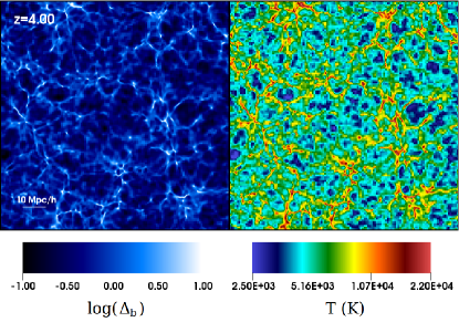
Figure 2: Overdensity (left) and temperature (right) distribution in a slice of the L1 simulation at $z=4$.

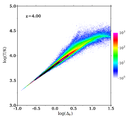
Figure 3: Temperature–density relation for low-density IGM in the L1 simulation at $z=4$ when the volume filling factor of He iii is less than $0.1$ per cent. The colour scale indicates the gas mass per pixel (in arbitrary units normalized to 1000 at maximum). Overplotted contours correspond to 10, 30, 50, 70 and 90 per cent of the maximum value. Note that the different levels are hardly distinguishable as most of the gas follows a very tight temperature–density relation.

At low densities, the IGM shows a tight temperature–density relation (see Fig. 3) determined primarily by the balance between photoheating, adiabatic cooling/heating and Compton cooling (e.g. Miralda-Escudé & Rees, 1994; Hui & Gnedin, 1997). As a result of these effects, we can write an ‘effective equation of state’ of the form

$$T=T_{0}\,\Delta_{\textrm{b}}^{\gamma-1},$$ (3)

where the gas temperature at mean density, $T_{0}\simeq 6300\,\textrm{K}$, and the polytropic index, $\gamma\simeq 1.56$, are determined by the cosmological model and the ionization history of the gas. The scatter around this relation is very small, i.e. the rms temperature variation at $\Delta_{\textrm{b}}=1$ is $\sigma_{0}\simeq 140\,\textrm{K}$.

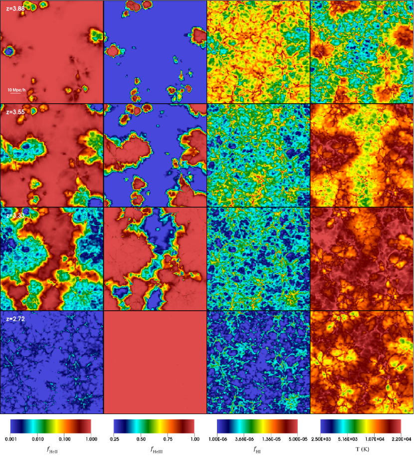
Figure 4: Slices through the L1 simulation. Each column refers to a different physical quantity: the fraction of singly ionized helium ($f_{\textrm{He\,{ii}}}$, left), the fraction of He iii  ($f_{\textrm{He\,{iii}}}$, centre left), the fraction of neutral hydrogen ($f_{\textrm{H\,{i}}}$, centre right) and the IGM temperature (right). Each row, instead, corresponds to a different stage of He ii reionization at redshift 3.88 (top), 3.55 (top-centre), 3.33 (bottom-centre) and 2.72 (bottom) corresponding to an He iii filling factor, $f_{\textrm{He\,{iii}}}$, of $0.10,\leavevmode\nobreak\ 0.51,\leavevmode\nobreak\ 0.80$ and $\leavevmode\nobreak\ 0.99$, respectively.

3.2 Reionization history

A cartoon sketching the propagation of ionizing radiation from AGNs through the L1 simulation is shown in Fig. 4. This refers to the same slice presented in Fig. 2. Each row corresponds to a given epoch ($z=3.88,3.55,3.33$ and $2.72$ from top to bottom) and is characterized by a specific value of the total He iii filling factor ($0.10,0.51,0.80$ and $0.99$, respectively). On the other hand, each column refers to a different property of the IGM (from left to right: the He ii fraction, the He iii fraction, the H i fraction and the gas temperature).

When an AGN turns on in a medium devoid of He iii, it carves during its lifetime an He iii region in the IGM with a characteristic size of several $h^{-1}\textrm{Mpc}$ (depending on the luminosity of the ionizing source) before switching off. The ionized bubbles have irregular shapes mainly determined by the underlying distribution of matter. Ionization fronts propagate faster at low densities, where the time-scale for recombination is larger, and thus rapidly sweep the volume-filling underdense regions. At first, He iii bubbles are well separated by extended He ii regions. When their central source switches off, the internal He iii fraction decreases due to recombinations until a new AGN becomes active in the surroundings. After different generations of AGNs have shined, bubbles overlap and the He iii phase percolates. At this point, the topology of the different ionized states of helium has reversed: small pockets of He ii – which are shielded from ionizing radiation by high-density clumps – emerge from an ‘ocean’ of He iii.

	$f_{\textrm{He\,{iii}}}\leq 0.1$			$f_{\textrm{He\,{iii}}}\geq 0.9$
$z$	$\gamma$	$\log(T_{0}/\textrm{K})$	Vol	$\gamma$	$\log(T_{0}/\textrm{K})$	Vol
$3.77$	$1.4412\pm 0.0001$	$3.8506\pm 0.0002$	$0.65$	$1.2625\pm 0.0001$	$4.1723\pm 0.0007$	$0.08$
$3.59$	$1.3568\pm 0.0001$	$3.9006\pm 0.0002$	$0.28$	$1.2408\pm 0.0001$	$4.1847\pm 0.0004$	$0.19$
$3.48$	$1.3148\pm 0.0001$	$3.9372\pm 0.0004$	$0.06$	$1.2104\pm 0.0001$	$4.2058\pm 0.0003$	$0.36$
$3.33$	$1.2834\pm 0.0003$	$3.9808\pm 0.0013$	$2\cdot 10^{-3}$	$1.1977\pm 0.0001$	$4.2145\pm 0.0003$	$0.61$
$3.15$	$1.42\pm 0.10$	$3.93\pm 0.21$	$5\cdot 10^{-5}$	$1.1958\pm 0.0001$	$4.2014\pm 0.0003$	$0.78$
$2.94$	$-$	$-$	$0$	$1.2048\pm 0.0001$	$4.1906\pm 0.0003$	$0.98$

Table 4: To emphasize and quantify the bimodal distribution of the gas temperature that forms during He ii reionization in the L1 simulation, we fit the temperature–density relation of highly ionized gas ($f_{\textrm{He\,{iii}}}\geq 0.9$) and lowly ionized gas ($f_{\textrm{He\,{iii}}}\leq 0.1$) in the density range $-1.5\leq\log(\Delta_{\textrm{b}})\leq 0.5$ with two separate power laws of the form given in Equation (3). The volume fraction in the two ionization states is also given.

Figure 5: Temperature evolution (red curve, left-hand axis) and evolution of the fraction of He ii (blue curve, right-hand axis) in terms of the simulation time for two different cells (top and bottom panels) at mean density in the L1 simulation.

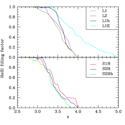
Figure 6: Redshift evolution of the He iii filling factor in our simulations. Top: L1 (green), L1b (black), L1E (cyan) and L2 (purple) simulations. Bottom: high-resolution regions probed by the S1H (red), S2H (blue) and S2Hb (green) volumes.

The passage of an ionization front is also associated with an increase in the temperature of the medium due to the thermalization of the photoelectrons. As an example, in Fig. 5 we show the evolution of the He ii fraction and of the gas temperature in two different cells at mean density in the L1 simulation. The top panel shows that helium is singly ionized at a temperature of $T\sim 6400\,\textrm{K}$ when a front reaches the cell. The He ii fraction rapidly decreases and the transition to a completely ionized state requires $\sim 250\,\textrm{$\textrm{Myr}$}$. Since this time exceeds the lifetime of a single AGN, the ionization process takes place because of the contribution of multiple sources that switch on at different times. A consequence of this phenomenon is evident in the figure: at the simulation time of $\sim 100$ Myr, a nearby source switches off. Both the temperature and the He ii fraction thus reach a plateau that lasts for a few Myr, i.e. until the ionizing photons from other sources reach the cell . Later on, ionization equilibrium is established and the temperature reaches a maximum value of $T\sim 17\kern 1.66672pt000\,\textrm{K}$. After the front has swept the cell, the temperature decreases monotonically according to Hubble cooling with a time-scale of $\sim 1$ Gyr. The bottom panel of Fig. 5 depicts a similar scenario where the contribution from multiple sources is necessary to completely ionize the cell.

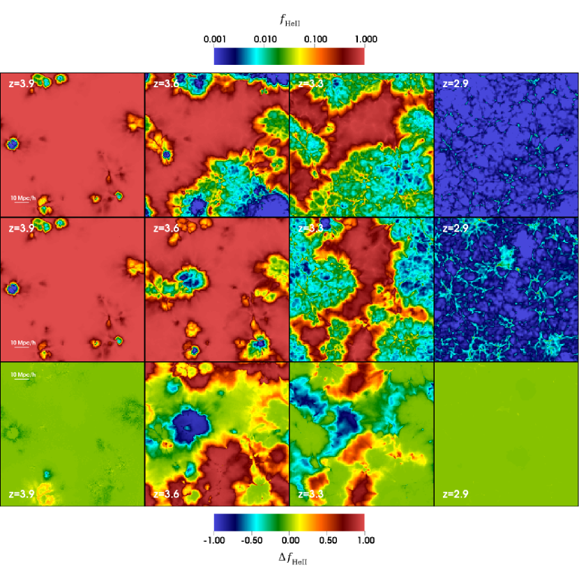
Figure 7: Comparison between the source models adopted in the L1 and L2 simulations at different redshifts (as indicated in the labels). Top: distribution of the He ii fraction in a slice from the L2 simulation. Centre: distribution of the He ii fraction in a slice of the L1 simulation as also shown in Fig. 4. Bottom: difference between the He ii fractions in the L1 and L2 simulations, $\Delta f_{\textrm{He\,{ii}}}=f_{\textrm{He\,{ii}}}^{\textrm{(L1)}}-f_{\textrm{He\,{ii}}}^{\textrm{(L2)}}$. Note that, to ease comparison, both simulations start with the same distribution of sources at $z=4$.

In Fig. 6, we show the time evolution of the He iii filling factor in the simulations. In the L series, the filling factor approaches unity between $2.9\lesssim z\lesssim 3.1$, in good agreement with high-quality Cosmic Origin Spectrograph observations (e.g. Shull et al., 2010; Worseck et al., 2011). Even in the L1b box, where He reionization proceeds at a faster pace due to the presence of very luminous sources, the fraction of He ii drops below $1$ per cent only at $z\simeq 3.0$, analogously to what happens in the L1 and L2 simulations. Overall, He ii ionization and the corresponding heating of the IGM are extended processes that take place within a redshift interval $\Delta z\gtrsim 1$ in line with the observational evidence based on the curvature of quasar absorption lines presented in Becker et al. (2011). This result is even more evident in the L1E simulation where the He iii filling factor at $z=4$ is equal to $0.425$ but the reionization is completed only at $z<3.4$.

Additional insight on how He ii reionization takes place at a local level is provided by the S simulations. In fact, the S1H, S2H and S2Hb boxes provide us with a few realizations of a small portion of the Universe, characterized by different reionization histories. The detailed evolution of the He iii filling factor depends on the actual distribution of AGNs around and within the boxes. For instance, at $z\sim 3.8$ roughly $20$ per cent of He in the S1H volume is already fully ionized while in the S2Hb box $f_{\textrm{He\,{iii}}}<0.05$.

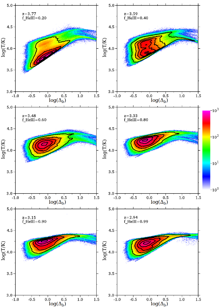
Figure 8: Evolution of the temperature–density relation during He ii reionization in the L1 simulation. The style of the plot is as in Fig. 3.

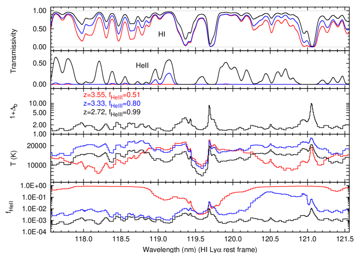
Figure 9: Typical H i and He ii Ly$\alpha$ absorption spectra along a line of sight extracted from our L1 simulation for three different redshifts: $z=3.55$ (red), $3.33$ (blue) and $2.72$ (black). From top to bottom, we show, respectively: the H i and He ii transmitted flux (both convolved with a Gaussian profile with a FWHM of $88\,\textrm{$\textrm{km}\,\textrm{s}^{-1}$}$), the gas overdensity, the gas temperature and the fraction of singly ionized helium, $f_{\textrm{He\,{ii}}}$. The wavelength along the $x$-axis has been rescaled to the H i Ly$\alpha$ transition in the rest frame of the gas appearing at the extreme right of the plot.

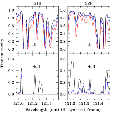
Figure 10: Sample H i and He ii Ly$\alpha$ absorption spectra along a line of sight extracted from the S1H (left) and the S2H (right) simulations at different redshifts: $z=3.5$ (red), $3.2$ (blue) and $2.9$ (black). The synthetic spectra have been convolved with a Gaussian profile with a FWHM of $12\,\textrm{$\textrm{km}\,\textrm{s}^{-1}$}$.

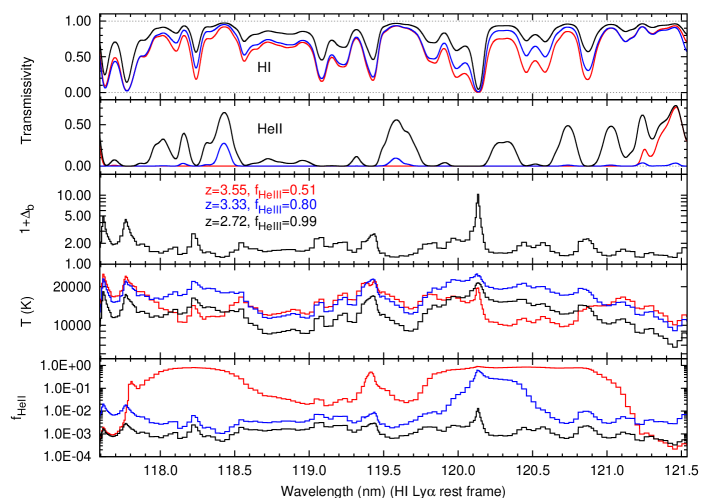
Figure 11: As in Fig. 9 but along a particular line of sight which has impact parameters $\simeq 4.7$ and $\simeq 7.2\,\textrm{$h^{-1}\textrm{Mpc}$}$ with respect to a pair of closely spaced ($\sim 4.2\,\textrm{$h^{-1}\textrm{Mpc}$}$) sources active between $z=3.6$ and $3.52$ with magnitude $M_{1450}\simeq-22.4$ and $-22.9$, respectively. An intense transmission peak in the He ii spectrum is evident around $\lambda\simeq 121.4\leavevmode\nobreak\ \textrm{nm}$ both at redshift $z=3.55$ and $2.72$ while it is not present at intermediate redshifts.

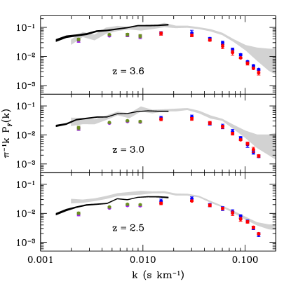
Figure 12: Line-of-sight power spectrum of the H i transmitted flux at different redshifts. Points with $1\sigma$ error bars have been extracted from our simulations and different colours refer to the various computational boxes: L1 (green), L2 (purple, hardly visible because almost perfectly overlapping with the green points), S1H (red) and S2H (blue). The shaded regions mark the observational constraints by McDonald et al. (2006, black) and Croft et al. (2002, grey).

Contrary to the global ionization history, the detailed geometry of the reionization process (e.g. the size of the ionized bubbles and their spatial distribution) depends on the model which is adopted for the evolution of the ionizing sources. This is emphasized in Fig. 7, where we compare the He ii distribution in the same slice of the L1 and L2 simulations as a function of redshift.

The PLE model, which contains fewer but more luminous sources at $z<4$, at early times presents on average more extended ionization fronts than the PDE model, which is characterized by smaller and more numerous ionization bubbles. During the initial stages of the reionization process the discrepancies are due to the properties and the location of the active sources at that particular time step. At later times, when the bubbles start percolating, the differences between the two models are less evident, as shown in the third column of Fig. 7. Both scenarios end up producing nearly complete He ii ionization at $z\sim 2.9$.

3.3 Temperature–density relation

Line-fitting studies of absorption features in quasar spectra indicate that the temperature–density relation of the IGM is characterized by a ‘normal’ equation of state with $\gamma>1$ (Bryan & Machacek, 2000; Ricotti et al., 2000; Schaye et al., 2000; McDonald et al., 2001; Zaldarriaga et al., 2001; Rudie et al., 2012). On the contrary, using the probability density function (PDF) of the transmitted flux, wavelet analysis, or a combination of both, other authors find evidence for an ‘inverted’ equation of state with $\gamma<1$ (Bolton et al., 2008; Viel et al., 2009; Calura et al., 2012; Garzilli et al., 2012).

In Fig. 8, we show how the temperature–density relation of the IGM is altered as He ii reionization progresses in the L1 box. As discussed above, gas elements are rapidly heated when they are invested by a photoionization front. Therefore, while He ii reionization is ongoing, an ever increasing fraction of gas leaves the original temperature–density relation and form a new, hotter and less tight sequence ($\sigma_{0}\simeq 3300\,\textrm{K}$ at $z=3.5$). As reionization proceeds, two well-defined and unequally populated $T$–$\Delta_{\textrm{b}}$ relations are present. We fit two different polytropic relations in the density interval $-1.5\leq\log(\Delta_{\textrm{b}})\leq 0.5$ by separately considering gas elements with a low ($f_{\textrm{He\,{iii}}}\leq 0.1$) and a high ($f_{\textrm{He\,{iii}}}\geq 0.9$) level of ionization. The best-fitting values for $\gamma$ and $T_{0}$ are reported in Table 4 together with the volume fraction of the gas in the two ionization states for all the redshifts appearing in Fig. 8. Eventually, when reionization is complete at $z\simeq 2.9$, a new $T$–$\Delta_{\textrm{b}}$ relation emerges with a value of $\gamma\simeq 1.20$ which is smaller than the initial one. At this time the gas temperature at mean density is $T_{0}\sim 15\kern 1.66672pt600\,\textrm{K}$ and the rms temperature variation decreases to $\sigma_{0}\simeq 2800\,\textrm{K}$. At low densities, we find no evidence for an inverted equation of state of the IGM (e.g. $\gamma<1$) while we detect it for early times and $\Delta_{\rm b}>10$ as expected from arguments of thermal balance (e.g. Meiksin, 1994; Miralda-Escudé & Rees, 1994; Tittley & Meiksin, 2007; Meiksin & Tittley, 2012).

3.4 Simulated spectra

We produce mock Ly$\alpha$ absorption spectra based on the distribution and velocity of H i and He ii along different lines of sight in our computational volumes. We use resolution elements of $1\,\textrm{$\textrm{km}\,\textrm{s}^{-1}$}$ and select lines of sight which are parallel to one of the main axes of the computational box. In order to mimic the instrumental response of a real spectrograph, we convolve each spectrum with a Gaussian profile. For the S1H, S2H and S2Hb boxes, we use a kernel with a full width at half-maximum (FWHM) of $12\,\textrm{$\textrm{km}\,\textrm{s}^{-1}$}$. On the other hand, we adopt $88\,\textrm{$\textrm{km}\,\textrm{s}^{-1}$}$ for the L1, L1b, L1E, L2 and LHO simulations which have lower spatial resolution. In the latter case, our synthetic spectra are not able to resolve single H i lines of the Ly$\alpha$ forest but still give information on the coarse-grained properties of the medium.

Sample spectra corresponding to the same line of sight in the L1 simulation at different redshifts are shown in Fig. 9. To ease the comparison, wavelengths are given for the H i Ly$\alpha$ transition in the rest frame of the gas that appears at the extreme right of the plot. Together with the H i and the He ii absorption spectra, the density, temperature and He ii ionization fraction of the gas are also displayed. Since we perform the radiative transfer in post-processing on a single snapshot of the AMR simulations, the density field evolves simply as $(1+z)^{3}$ and overdensities do not change. On the other hand, temperatures vary with time showing the expected behaviour: the passage of an He ii ionization front rapidly heats up the medium that then smoothly cools down. Overall, helium second ionization makes the IGM less opaque to both H i and He ii Ly$\alpha$ photons. As expected, the spectra of the two elements present some qualitative differences. In the redshift range, $3.55<z<2.72$, H i spectra show a constant increase in the transmitted flux but preserve the same pattern of absorption features. On the contrary, He ii spectra show a much more dramatic change transiting from complete absorption (at $z=3.55$) to the appearance of small regions of transmitted flux (at $z=3.33$) that subsequently increase in size and number as He ii reionization proceeds. Spectra obtained in the S1H and S2H volumes present similar features but resolve single H i absorption lines, as shown in Fig. 10.

In Fig. 11, we focus on a particular line of sight in the L1 simulation which has been selected because of its vicinity to a pair of closely spaced ($\sim 4.2\,\textrm{$h^{-1}\textrm{Mpc}$}$) luminous sources. It has an impact parameter of $\simeq 4.7\,\textrm{$h^{-1}\textrm{Mpc}$}$ with respect to a source with magnitude $M_{1450}\simeq-22.4$ and $\simeq 7.2\,\textrm{$h^{-1}\textrm{Mpc}$}$ with respect to a second AGN with magnitude $M_{1450}\simeq-22.9$ that are active between $z=3.60$ and $3.52$. For this reason, at redshift $z=3.55$ (red line), a transmission peak in the He ii spectrum is present around $\lambda\simeq 121.4\leavevmode\nobreak\ \textrm{nm}$. After the sources switch off, He iii starts recombining, thus reducing the transmissivity in the spectrum. In the absence of additional sources of ionizing radiation in the surroundings, the medium recombines enough to produce an almost complete absorption. This effect occurs at $z=3.33$ (blue line) when the transmission peak is extremely weak. Only at $z=2.72$, when reionization is completed, the fraction of He ii is again small enough to allow some flux to be transmitted. We will discuss extensively the implications of this kind of features in Section 4.3.

3.4.1 Flux power spectrum

Line-of-sight power spectra of the H i transmitted flux extracted from our simulations are shown in Fig. 12 together with the observational data by McDonald et al. (2006) and Croft et al. (2002). Our results are in qualitative agreement with observations and reproduce the expected shape of the power spectrum at all redshifts. The overall amplitude of the simulated spectra slightly underestimates the observational results. This might be a consequence of the fact that our S boxes are mildly underdense while hydrogen in the L boxes tends to be slightly more ionized than expected (see Section 4.1). Note that the L1 and L2 boxes produce nearly identical power spectra as the differences in their AGN models do not affect the largest scales.

4 GLOBAL REIONIZATION SIGNAL

4.1 Effective optical depth

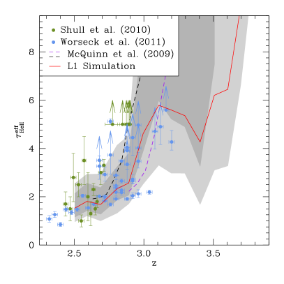
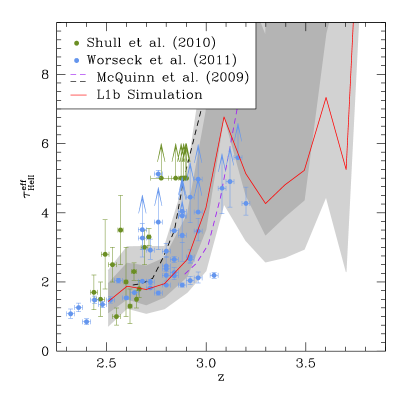
Figure 13: Redshift evolution of the mean He ii effective optical depth (red line) evaluated in identical bins of $\Delta z=0.04$ in the L1 (left) and L1b (right) simulations. Shaded areas denote the regions of the $\tau_{\textrm{He\,{ii}}}^{\textrm{eff}}$ distribution enclosed between the $16\textrm{th}$ and $84\textrm{th}$ percentile (dark grey) and between the $2\textrm{nd}$ and $98\textrm{th}$ percentile (light grey). Observational data by Shull et al. (2010) (green points, $\Delta z=0.1$) and Worseck et al. (2011) (blue points, $\Delta z=0.04$) are overplotted for comparison. The dashed lines indicate the mean $\tau^{\textrm{eff}}_{\textrm{He\,{ii}}}$ extracted from the radiative-transfer simulations by McQuinn et al. (2009) (their L3 simulation is drawn in black and their D1 simulation in purple) as computed in Worseck et al. (2011) with $\Delta z=0.04$. The dip at $z\sim 3.4$ in the L1 volume is generated by a positive fluctuation in the total number of ionizing photons. Similarly, the L1b simulation presents a deficit of ionizing photons at $z\sim 3.1$ that momentarily increases the effective optical depth in the volume (see Appendix C for details).

In order to quantify the evolution in the transmissivity of the IGM and compare our simulations against observations, we compute the effective optical depth $\tau^{\textrm{eff}}=-\ln\langle F(z)\rangle_{\textrm{los}}$, where $F$ is the transmitted flux ($0\leq F\leq 1$) and the symbols $\langle\cdot\rangle_{\textrm{los}}$ denote the average over many lines of sight. In Figs 13 and 14, we show the mean He ii effective optical depth, $\tau^{\textrm{eff}}_{\textrm{He\,{ii}}}$, evaluated from $100$ random spectra in the L1, L1b and L2 simulations using spectral bins with a size of $\Delta z=0.04$ as in Worseck et al. (2011). Data obtained from observations of high-redshift quasars (Shull et al., 2010; Worseck et al., 2011) and simulations (McQuinn et al., 2009, as computed in Worseck et al., 2011 with bins $\Delta z=0.04$) are also displayed for comparison. For $z<3.2$, our results lie in the same ballpark as the experimental data. At higher redshifts, not yet probed by observations, the effective optical depth in the L1, L1b and L2 simulations presents strong oscillations connected to the fluctuating number of ionizing photons in the volumes. Note that the skewness of the distribution of $\tau^{\textrm{eff}}_{\textrm{He\,{ii}}}$ implies that the evaluation of the mean optical depth is mostly influenced by those regions of He ii spectra with lower opacity therefore the mean is substantially different from the median. Our results for $\tau^{\textrm{eff}}_{\textrm{He\,{ii}}}$ are in good agreement with those presented by McQuinn et al. (2009) at low redshifts ($z<3$) especially once the uncertainties of the models are taken into account, but in our simulations $\tau^{\textrm{eff}}_{\textrm{He\,{ii}}}$ increases more gradually at higher redshifts. We do not show analogous results from the S boxes because of the limited wavelength range covered by these simulations which corresponds to $\Delta z\simeq 0.02$.

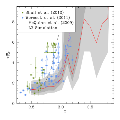
Figure 14: As in Fig. 13 but for the L2 simulation.

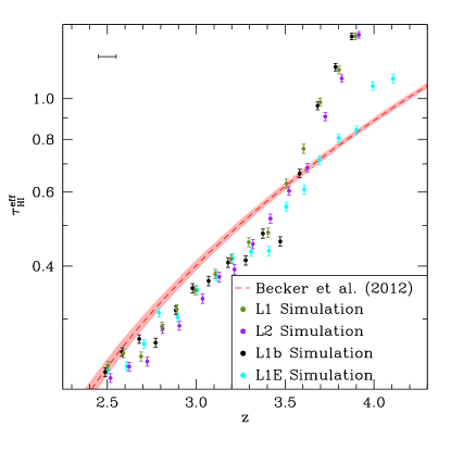
Figure 15: Redshift evolution of the H i effective optical depth in the L1 (green), L1b (black), L2 (purple) and L1E (cyan) simulations evaluated using bins of $\Delta z=0.1$ (as indicated by the horizontal error bar in the top-left corner of the plot). The analytic fit to observational data (red dashed line) by Becker et al. (2012) together with their $1\sigma$ uncertainty (shaded region) are also reported for comparison. Data from the L1b and L2 simulations have been slightly shifted in redshift ($-0.02$ and $+0.02$, respectively) to ease readability. Error bars indicate the standard error of the mean.

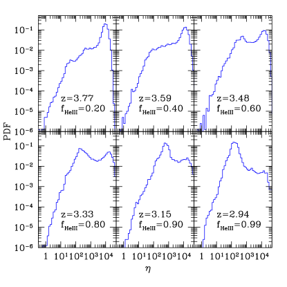
Figure 16: PDF of the column-density ratio $\eta=\frac{N_{\textrm{He\,{ii}}}}{N_{\textrm{H\,{i}}}}$ at different redshifts from $100$ lines of sight in the L1 simulation.

In Fig. 15, the H i effective optical depth, $\tau^{\textrm{eff}}_{\textrm{H\,{i}}}$, evaluated from our L volumes is compared with the most recent measurements of the mean transmitted flux in the Ly$\alpha$ forest by Becker et al. (2012):

$$\tau^{\textrm{eff}}_{\textrm{H\,{i}}}(z)=\tau_{0}\left(\frac{1+z}{1+z_{0}}\right)^{\beta}+C,$$ (4)

with $z_{0}=3.5$, $\tau_{0}=0.751$, $\beta=2.90$ and $C=-0.132$. At $z>3.7$, the effective optical depth in the L1, L1b and L2 simulations is higher than observed and shows a steep evolution. This is not surprising since we start our radiative-transfer calculations in these volumes at $z_{\textrm{AGN}}=4$ and no AGN contribution to the UV background has been considered before. In fact, measurements of the effective optical depth in the L1E simulation show a better agreement with the observed $\tau^{\textrm{eff}}_{\textrm{H\,{i}}}$ already at $z\simeq 3.9$. For $2.5<z<3.7$, the effective optical depth for all simulated volumes departs by less than 10 per cent from the observational results even though it tends to be systematically lower. This is remarkable as we do not need to artificially rescale the H i optical depth of our spectra to match observations as often done in the literature.

4.2 The He ii/H i column-density ratio

Absorption features in H i and He ii spectra trace the same underlying density field. Therefore, the ratio of the column densities $\eta=N_{\textrm{He\,{ii}}}/N_{\textrm{H\,{i}}}$ tracks the ratio of ionizing fluxes at $1$ and $4\,\textrm{ryd}$ and can be considered a measurement of the hardness of the UV background. Fig. 16 presents the PDF of $\eta$ along $100$ lines of sight at different redshifts in our L1 simulation. Instead of fitting Voigt profiles to the mock spectra, the value of $\eta$ is obtained directly from the ratio of the number densities in each cell of the simulation. This way we can also probe optically thick regions. At high redshift, the distribution is dominated by a single peak at $\eta\simeq 10^{4}$, corresponding to spectra where the He ii flux is highly absorbed while the H i spectra show some transmission. As He ii reionization progresses, a second peak between $\eta\simeq 10^{2}$ and $10^{3}$ forms due to the increasing AGN contribution to the UV background. When the reionization is close to completion ($z\simeq 2.9$), only the broad peak centred at $\eta\simeq 100$ is present: by this time, the UV background is completely dominated by the AGN contribution. Finally, at $z<2.7$ (not shown in the figure) $\eta$ shows a small scatter around a central value of $\sim 50$ and is never larger than a few hundred. Current observations are likely able to identify only the peak at low $\eta$. In fact, complete absorption in He ii (within the noise level) precludes precise measurements of very large values of $\eta$. Only lower limits can be given in this situation. Note that at high redshift, some cells in our simulations are characterized by a value of $\eta$ smaller than unity.

4.3 Flux-transmission windows and dark gaps

At high redshift, the regions of transmitted flux in He ii spectra are relatively narrow in wavelength and are clearly bounded by complete absorption. In the following, we will refer to each of these regions as a ‘Flux-Transmission Window’ (FTW). We operatively define an FTW as a region in the He ii spectrum where the flux is above $0.2$ times the continuum level. Within the local Gunn–Peterson approximation, a $1$ per cent fraction of singly ionized helium is enough to completely saturate, with $\tau\gg 10$, the Ly$\alpha$ absorption, even in the underdense regions where $\Delta_{\textrm{b}}\simeq 0.1$. Therefore, we expect to detect FTWs only if the medium is very highly ionized and the recombination time is sufficiently long. Our simulations reveal that, depending on redshift and the extent of the ionization fronts, FTWs can occupy mildly overdense regions surrounding AGNs or can be found in low-density environments, even at large distances from any source of ionizing photons.

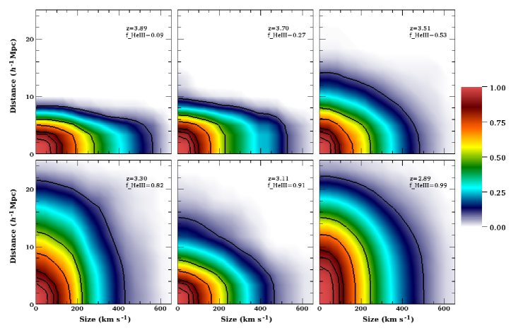
Figure 17: Bivariate cumulative distribution function for the FTW size (in $\textrm{km}\,\textrm{s}^{-1}$) and the distance (in $h^{-1}\textrm{Mpc}$) from the nearest source computed using $2500$ spectra extracted from the L1 simulation (PLE model). Contour levels enclose $5$, $10$, $15$, $30$, $50$ and $90$ per cent of the total number of points.

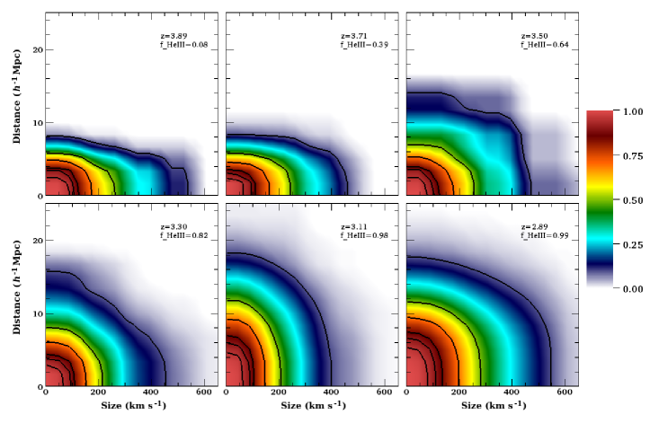
Figure 18: As in Fig. 17 but for the L2 simulation (PDE model).

In Figs 17 and 18, we present the cumulative joint distribution of the FTW size (in $\textrm{km}\,\textrm{s}^{-1}$) and of the distance from the nearest active source (in $h^{-1}\textrm{Mpc}$) in the L1 and L2 simulations. The colour of the pixel located at coordinates $(x,y)$ describes the probability that an FTW has size greater than $x$ and distance $y$ or higher from an active source. The PDE and PLE models produce very similar results at all redshifts. At the onset of He ii reionization, spectra from the L1 and L2 simulations are characterized by extended ($\sim 300\,\textrm{$\textrm{km}\,\textrm{s}^{-1}$}$) FTWs at moderate distance from the ionizing sources. However, no FTWs appear at distances $>10\,\textrm{$h^{-1}\textrm{Mpc}$}$ from any AGN. As reionization proceeds, the size of the transmission windows evolves only marginally, while more and more FTWs can be found at large distances from the nearest active source. When He ii reionization is completed, FTWs typically extend for $\sim 250\,\textrm{$\textrm{km}\,\textrm{s}^{-1}$}$, with a characteristic distance from the nearest active source of $\simeq 15\,\textrm{$h^{-1}\textrm{Mpc}$}$ for the L1 simulation and $\simeq 12\,\textrm{$h^{-1}\textrm{Mpc}$}$ for the L2 volume. A transient feature is seen in the L1 box around $z=3.1$ and is related to a negative fluctuation in the number of ionizing photons in the simulation (see Appendix C). The properties of the FTWs strictly correlate with the spectral characteristics of the active sources and do not depend on the past ionization history of the medium. Only sources undergoing an active phase leave a detectable imprint on the IGM, even during the last stages of the reionization, when the medium is expected to be less influenced by the adopted AGN model.

At redshift $z\gtrsim 3.5$, regions with a low optical depth in the Ly$\alpha$ forest are very rare. An alternative method to analyse the statistical properties of He ii spectra is the distribution of dark gaps in the transmitted flux. We operationally define a dark gap as a region in the He ii spectrum where the flux is below 20 per cent of the continuum level. Figs 19 and 20 show the evolution with redshift of FTWs and dark gaps in the L1 and L2 simulations, compared with the homogeneous reionization scenario provided by the LHO simulation. Data are extracted from $2500$ spectra taken along random lines of sight. The characteristic size of the FTWs presents a similar evolution with redshift in the L1 and L2 simulations. Minor differences can be related to fluctuations in the number of ionizing photons in the two volumes. At $z\geq 2.8$, the number density of FTWs per unit redshift comes out to be a promising statistic to investigate the degree of patchiness of He ii reionization: in the PLE and PDE models, this quantity is more than one order of magnitude larger than what is expected for a reionization scenario with homogeneous UV background. Note that for $z>3.1$ no FTWs are detected in the homogeneous-reionization run where the He ii effective optical depth is slightly higher than what is found with observations.

At later times, when He ii ionization is nearly complete, both inhomogeneous models and the homogeneous reionization produce a comparable number of FTWs. On the other hand, the number density of dark gaps (Fig. 20) presents only small deviations between the different reionization scenarios at high redshifts. However, as it might be expected, the median length of the dark gaps in the PLE and PDE scenarios drops to $\sim 1000$ $\textrm{km}\,\textrm{s}^{-1}$ much earlier than in the homogeneous case. Note that the properties and the distribution in size of FTWs and dark gaps are only marginally influenced by the adopted inhomogeneous model: evolving with redshift the luminosity or the number density of the sources of ionizing radiation does not produce significant differences in the FTWs and dark gaps statistics, once random fluctuations in the number of ionizing photons are taken into account.

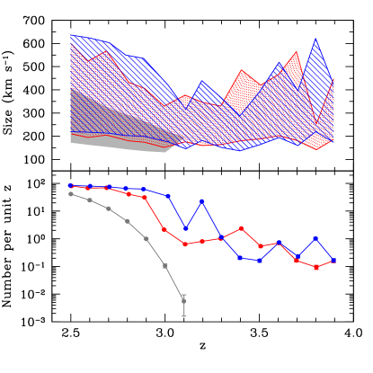
Figure 19: Comparison between the FTWs in 2500 He ii spectra generated by different reionization scenarios. Top: characteristic size of the FTWs in the L1 (red), L2 (blue) and LHO (grey) simulations. The shaded area marks the region enclosed between the first and the third quartile. Bottom: number density of FTWs per unit redshift (error bars show the standard error of the mean). We neglect FTWs with size smaller than $88\,\textrm{$\textrm{km}\,\textrm{s}^{-1}$}$, corresponding to the nominal resolution of our simulations. No FTWs are detected for $z>3.1$ in the LHO box.

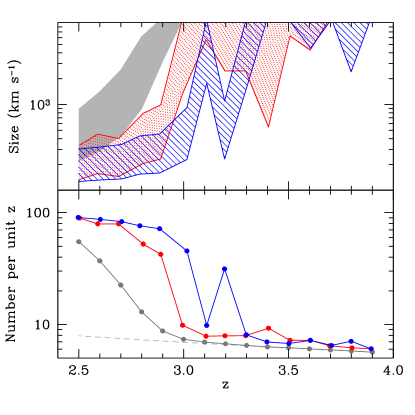
Figure 20: As in Fig. 19 but for the dark gaps. Note that the top panel shows the range between the median and the $10^{\textrm{th}}$ percentile. The dashed line represents the minimum number of dark gaps that can be detected in our volume (one per line of sight).

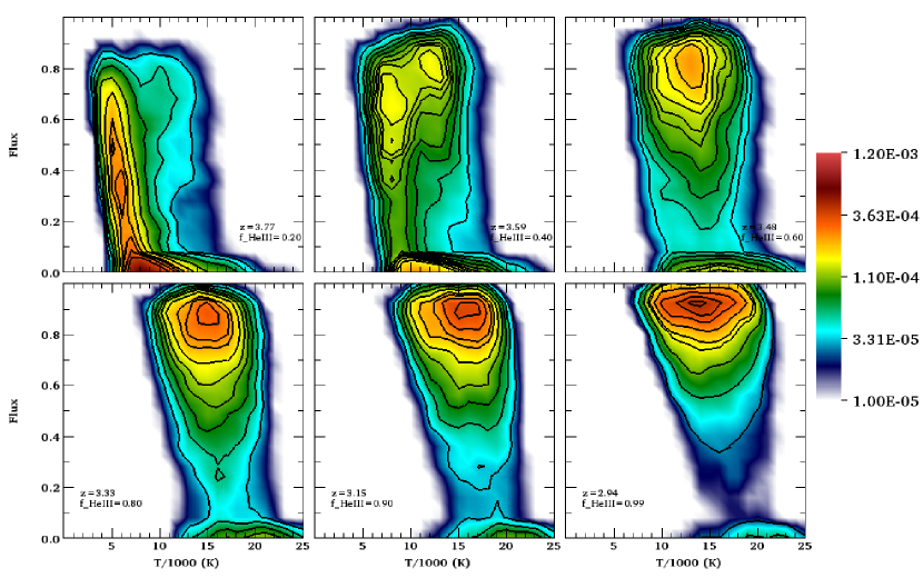
Figure 21: Bivariate joint-probability density (in $\textrm{K}^{-1}$) of the temperature and the corresponding H i transmitted flux measured from $100$ simulated spectra in the L1 simulation. Contour levels enclose from 10 to 90 per cent probability in steps of 10 per cent.

5 PROBING THE LOCAL IONIZATION HISTORY

5.1 Temperature bimodality

During the initial stages of He ii ionization, the IGM can be envisaged as being composed of two phases (see Fig. 8): at fixed density, hot, already ionized patches can be identified around the locations where AGNs have been shining while regions that have never been crossed by ionization fronts tend to be colder. This temperature bimodality at fixed density leaves an imprint in quasar spectra. In Fig. 21, we present the joint probability distribution of the temperature and the H i transmitted flux (the matching is made at fixed wavelength in the spectra as in Fig. 9) obtained considering $100$ random sightlines in the L1 simulation. At the onset of helium reionization ($z\simeq 4$), characteristic temperatures scatter around $T\simeq 6\times 10^{3}\,\textrm{K}$ and the flux transmissivity is limited to less than a few tens of per cent. However, when the He iii filling factor reaches 40 per cent or so, a strong bimodal behaviour is established: high transmissivity tends to be associated with high-temperature elements, while higher opacity corresponds to lower temperatures. At later times, when $f_{\textrm{He\,{iii}}}\geq 0.6$, the distribution becomes again unimodal and is characterized by hot gas and relatively large transmissivity. When the reionization is complete, the gas progressively cools down to lower temperatures.

It is not trivial to make a connection between Figs 8 and 21. One needs to relate the gas density to the transmitted flux. In Fig. 22, we show how the joint probability density of these quantities evolves during He ii reionization. The peak of the distribution progressively shifts towards lower overdensities and higher transmissivities with time. In other words, gas elements at fixed overdensity are associated with higher fluxes as reionization proceeds. At fixed transmitted flux, He ii reionization shifts the characteristic overdensity sampled by spectra towards higher $\Delta_{\textrm{b}}$ and $T$.

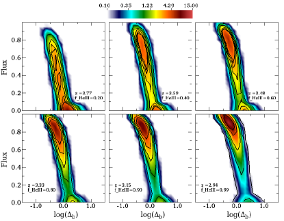
Figure 22: Bivariate joint-probability density of the baryonic overdensity and the H i transmitted flux. Contour levels enclose $50$, $60$, $70$, $80$ and $90$ per cent probability.

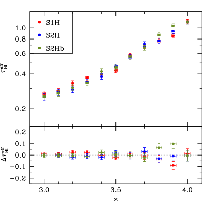
Figure 23: Top: H i effective optical depth in the S1H (red), S2H (blue) and S2Hb (green) volumes. Data have been obtained from $150$ spectra using bins of $\Delta z=0.02$. Error bars reflect the standard error of the mean flux. Bottom: difference between the effective optical depth evaluated in the S1H, S2H and S2Hb simulations and the mean of the three, $\Delta\tau_{\textrm{H\,{i}}}^{\textrm{eff}}=\tau_{\textrm{H\,{i}}}^{\textrm{S}_{\textrm{i}}}-\langle\tau_{\textrm{H\,{i}}}^{\textrm{eff}}\rangle$.

5.2 Observational probes of patchy reionization

As a consequence of the patchiness of He ii reionization, widely separated volume elements get ionized at slightly different times and this produces the above mentioned temperature bimodality of the IGM. Can high-resolution quasar spectra distinguish between He iii regions and volumes that have yet to be ionized? As an example, let us consider the two high-resolution simulations that differ most in the ionization history: in the S1H box, the volume filling factor of He iii reaches 20 per cent nearly $185\,\textrm{$\textrm{Myr}$}$ earlier than in the S2Hb volume (corresponding to $\Delta z\sim 0.35$, see Fig. 6). In Fig. 23, we compare the evolution of $\tau_{\textrm{H\,{i}}}^{\textrm{eff}}$ in the high-resolution boxes. The effective optical depth in the S1H simulation drops very rapidly when the volume is reached by ionization fronts and shows a milder evolution at later times. When this box is already substantially ionized at $z\simeq 3.9$, ionization fronts have yet to reach the S2Hb volume while the S2H simulation has an intermediate ionization state. At this point, the scatter in $\tau_{\textrm{H\,{i}}}^{\textrm{eff}}$ reaches a maximum. As reionization proceeds in all simulations, the evolution of the effective optical depth in the three volumes is very similar ($z\leq 3.7$), with small fluctuations related to the different properties of the ionizing sources in the boxes. All this suggests that an increased scatter in transmissivity between different lines of sight can be used as an indicator of the onset of He ii reionization.

In the remainder of this section, we investigate how a patchy reionization process and the temperature bimodality of the IGM make an impact on to different statistical probes that are commonly used to analyse the H i Ly$\alpha$ forest in quasar spectra. In order to resolve the scales associated with these absorption features we mainly focus on the high-resolution simulations S1H and S2Hb.

5.2.1 Distribution of the Doppler $b$ parameters

Using the VPFIT package, we fit multiple Voigt profiles to the mock H i absorption-line spectra extracted from the S1H and S2Hb simulations. In Fig. 24, we compare the cumulative distributions of the Doppler $b$ parameters measured in the two simulations. Only absorption lines with low column density, $\log{N_{\textrm{H\,{i}}}}<14.0\,\textrm{cm}^{-2}$, and a small error on the $b$ parameter, $\Delta b<10\,\textrm{$\textrm{km}\,\textrm{s}^{-1}$}$, are considered. We report in the figure also the probability that the two samples are extracted from the same parent distribution according to the Kolmogorov–Smirnov statistics ($P_{\rm ks}$). The difference between the distributions becomes statistically significant (at the $95$ per cent confidence level) at $z=3.9$ and increases even further at $z=3.8$, when the gas in the S1H box is being heated by the ionization fronts while the He iii filling factor in the S2Hb volume is still smaller than a few per cent. The maximum discrepancy between the cumulative distributions is recorded for $b\simeq 56\,\textrm{$\textrm{km}\,\textrm{s}^{-1}$}$. Later on, as He ii reionization proceeds also in the S2Hb volume, the distributions become more and more similar. This analysis shows that the Doppler parameter of lines with low column density is very sensitive to the temperature increase associated with the initial stages of the reionization process. During the initial phases of He ii reionization the mean and the standard deviation of the $b$ parameter distribution move from $50.5\pm 29.2\,\textrm{$\textrm{km}\,\textrm{s}^{-1}$}$ (with a median of $\simeq 43.2\,\textrm{$\textrm{km}\,\textrm{s}^{-1}$}$) to $55.8\pm 37.7\,\textrm{$\textrm{km}\,\textrm{s}^{-1}$}$ (with a median of $\simeq 45.1\,\textrm{$\textrm{km}\,\textrm{s}^{-1}$}$) as seen in observations for higher column densities (Rauch, 1998).

5.2.2 The curvature statistic

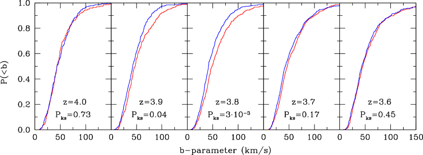
Figure 24: Cumulative distributions of the Doppler $b$ parameters for Ly$\alpha$ lines with H i column density $\log(N_{\textrm{H\,{i}}})<14.0\,\textrm{cm}^{-2}$ and statistical error $\Delta b<10\,\textrm{$\textrm{km}\,\textrm{s}^{-1}$}$. Data extracted from $150$ spectra in the S1H and S2Hb volumes are plotted in red and blue, respectively. The probability that the two samples are extracted from the same parent distribution according to the Kolmogorov–Smirnov test is given in each panel together with the corresponding redshift.

An alternative method that has been proposed to measure the imprint of He ii ionization on the IGM is the curvature statistic. This is defined in terms of the transmitted H i flux, $F_{\textrm{H\,{i}}}$, as (Becker et al., 2011)

$$\kappa\equiv\frac{F^{\prime\prime}_{\textrm{H\,{i}}}}{\left[1+(F^{\prime}_{\textrm{H\,{i}}})^{2}\right]^{3/2}}\,,$$ (5)

where the prime denotes differentiation with respect to the velocity separation in the spectrum. The curvature essentially coincides with $F^{\prime\prime}_{\textrm{H\,{i}}}$ as the denominator in Equation (5) is always very close to unity. This statistic does not require the decomposition of the Ly$\alpha$ forest into single absorption features and is thus suitable also when the absorption lines are strongly blended. We consider $450$ mock absorption spectra extracted from the S1H and S2Hb simulations. In order to measure the curvature, we first fit each spectrum with a cubic spline and normalize the flux to the maximum value of the fit. The evolution with redshift of the mean absolute curvature, $\langle|\kappa|\rangle$, reproduces the trend seen in observational data (Becker et al., 2011) for $z<3.5$, as shown in Fig. 25 for the S1H volume. In Fig. 26, we compare the evolution with redshift of the mean absolute curvature evaluated in the S1H and in the S2Hb simulations. As soon as the He ii ionization fronts have swept a small fraction of the volume, the mean absolute curvature in the S1H box departs from the results in the S2Hb simulation, when considering bins of high transmissivity. Later on, when the local He iii filling factor in the S2Hb box increases ($z\leq 3.7$), the two distributions are again very similar. Although it is a small effect, the redshift evolution of $\langle|\kappa|\rangle$ might be able to identify the onset of He ii reionization. Probing different lines of sight, one should be able to distinguish regions with different ionization histories by measuring the mean absolute curvature in narrow redshift bins of high transmissivity. For instance, we expect that the temperature bimodality which arises in our models at $3.6<z<4.0$ should be reflected in a broad and possibly bimodal distribution of the mean absolute curvature in real data.

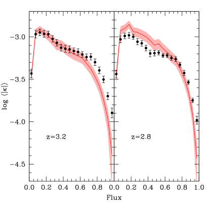
Figure 25: Distribution of the mean absolute curvature as a function of the normalized flux near the end of He ii reionization in the S1H simulation. The solid lines and the shaded regions show the values extracted from $450$ spectra and $2\sigma$ error bars, respectively. Points with error bars ($2\sigma$) are observational data from Becker et al. (2011).

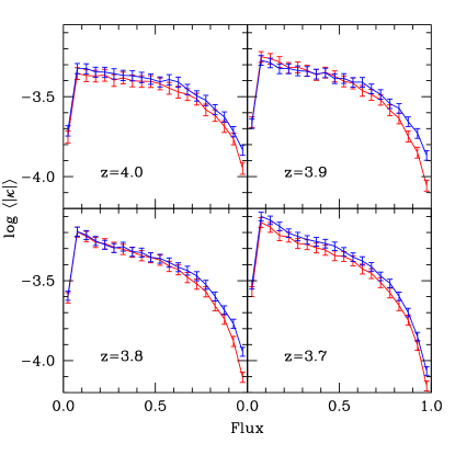
Figure 26: Evolution with redshift of the mean absolute curvature as a function of the normalized flux. The curvature is evaluated using $450$ spectra extracted from the S1H (red) and the S2Hb (blue) simulations. Error bars show the standard error of the mean.

6 CONCLUSIONS

We have investigated the epoch of He ii reionization using a suite of AMR hydrodynamic simulations with different box sizes. AGNs with a lifetime of $45\,\textrm{$\textrm{Myr}$}$ have been associated with dark matter haloes using a Monte Carlo method designed to reproduce the observed luminosity function at redshift $z=4$. For simplicity, the change in the AGN emissivity with time has been modelled assuming either pure density or pure luminosity evolution of the sources. Numerical radiative transfer of the ionizing radiation emitted by AGNs has been carried out in post-processing through a snapshot of the simulations. The UV emission by galaxies has been represented with a time-evolving but spatially uniform background.

We have studied how He ii reionization alters the thermal state of the IGM as well as its impact on the H i and He ii Ly$\alpha$ forest. Several statistics have been employed to probe into the topology of the reionization process in the redshift range $2.5<z<4$. Our main results can be summarized as follows.

1. In agreement with observations (Shull et al., 2010; Worseck et al., 2011), we find that He ii reionization is a process extended in redshift ($\Delta z\gtrsim 1$) characterized by a large sightline-to-sightline variance in He ii absorption. Well-separated ionized bubbles inflate around the location of the hard UV sources and start recombining when AGN activity terminates. Over time, bubbles percolate and the complete ionization of the IGM takes place. The He iii fraction and the temperature of the ionized IGM strongly correlate with the properties (luminosity and hardness) of the nearest AGNs, quickly losing memory of the previous ionization history of the gas. Within a single bubble, the gas properties are heterogeneous and depend on the underlying density distribution with a tight temperature–density relation. Small neutral islands form due to self-shielding of high-density regions which ionize last and reach the highest temperatures. The degree of patchiness in the He iii distribution is affected by the lifetime of the sources and the properties (number density and luminosity distribution) of the AGN population. On the other hand, the overall duration of the reionization epoch is rather model independent and only depends on the total emissivity of the UV sources.

2. The evolution of the H i and He ii effective optical depths in our simulations match data from high-resolution observations (e.g. Shull et al., 2010; Worseck et al., 2011; Becker et al., 2012). The He ii to H i column-density ratio, $\eta$, shows a strong spatial variability during He ii reionization and assumes values ranging between $0.5$ and $5\times 10^{4}$. Its PDF evolves with redshift reflecting the increasing volume fraction in which the UV radiation field is harder due to the AGN emission. The contribution of the ionized regions creates a peak at $\eta\simeq 50-100$ which becomes more and more prominent between $2.5<z<4$. This peak should be detectable from real data once a significant number of He ii quasars is available for spectral studies. In our simulations, the H i effective optical depth evolves smoothly during He ii reionization. In agreement with previous work (Bolton et al., 2009a, b; McQuinn et al., 2009), we do not recognize any sharp feature reminding of the narrow dip observed at $z\simeq 3.2$ (Theuns et al., 2002; Bernardi et al., 2003; Dall’Aglio et al., 2008; Faucher-Giguère et al., 2008). This is likely a consequence of the long duration of the reionization process.

3. The number density of the flux-transmission windows and the mean size of the dark gaps in the He ii spectra provide a powerful diagnostic tool to distinguish between different reionization scenarios (e.g. homogeneous versus inhomogeneous). Albeit these statistics encode information about the luminosity, number density and clustering properties of the sources responsible for reionization, they cannot discriminate between our PDE and PLE models. Fluctuations in the transmitted flux correlate with the local intensity of ionizing radiation. Very extended regions of transmitted flux are generally located next to bright AGNs even though there are rarer cases where flux-transmission windows with moderate size (100 $\textrm{km}\,\textrm{s}^{-1}$) can lie up to 22 $h^{-1}\textrm{Mpc}$ away from the nearest AGN.

4. The IGM is heated during He ii reionization: gas at mean density experiences a temperature jump of $\sim 12\kern 1.66672pt000\,\textrm{K}$ and cools afterwards. We find that the typical temperature increment from $z=4$ to $3$ (at mean density) ranges between $9000$ and $10\kern 1.66672pt000\,\textrm{K}$. This value is in good agreement with results based on the curvature of H i Ly$\alpha$ spectra (Becker et al., 2011).

5. The patchiness of the He ii reionization process gives rise to a bimodal distribution of the IGM temperature. Gas elements populate two distinct sequences in the temperature–density plane depending on their He iii fraction. At fixed density, ionized gas is hotter. The scatter around these effective equations of state is much smaller than the separation between the sequences. This is a transient feature which is particularly evident when $f_{\textrm{He\,{iii}}}\sim 0.4$. As reionization proceeds, more and more gas moves from the cold to the hot sequence. When He ii reionization is completed, only a single and well-defined temperature–density relation is present. At $z\simeq 2.9$, this is characterized by a polytropic index $\gamma\simeq 1.20$ which is lower than the corresponding value at the onset of reionization ($\gamma\simeq 1.56$). The average temperature at mean density is $T_{0}\simeq 1.56\times 10^{4}$ K, in agreement with observations (Becker et al., 2011) but slightly lower than in previous theoretical work (McQuinn et al., 2009; Meiksin & Tittley, 2012). We find no evidence for an inverted equation of state of the IGM at low densities $\Delta_{\rm b}<5$.

6. As a consequence of the bimodality in the temperature, neutral and ionized patches of the IGM are characterized by different probability distributions of the Doppler $b$ parameters and of the curvature of H i spectra. Therefore, we predict that He iii regions should generate H i spectra with higher $b$ parameters and a reduced mean absolute curvature in bins characterized by high transmissivity. These statistics are particularly sensitive during the initial stages of the reionization process, when the He iii volume filling factor is not too large.

This work presents a detailed theoretical study of the epoch of He ii reionization. Our analysis is based on the current understanding of the subject and uses the most advanced numerical tools. Many details of the model, however, are still prone to improvement. The properties of the sources of radiation and their time evolution, for instance, are still described with a toy model. Radiation transport is decoupled from hydrodynamic processes. In spite of this, our simulations provide a realistic description of the history of reionization which is compatible with all observational data. Our results, albeit more qualitative than quantitative, provide a starting point for novel investigations of the IGM. For instance, it would be interesting to analyse existing data on the H i forest at $3<z<4$ in light of the temperature bimodality seen in our simulations. Times are mature for investing in this challenge. In the next few years, studies of new sightlines towards He ii quasars will provide tighter constraints on many observables. At the same time, hydrodynamical simulations of cosmological volumes with increasing spatial resolution and more sophisticated radiative transfer (hopefully fully coupled to hydrodynamics) will become available. The reciprocal feedback between theory and observations will be key to shed new light on the physics of He ii reionization.

Appendix A Hydrodynamic Response

Our study is based on numerical simulations post-processed with a radiative-transfer code and thus neglects the hydrodynamical response of the gas to the heating due to He ii reionization. In order to estimate the accuracy of our approximations, we compare the output of two periodic AMR simulations with identical initial conditions. The first box (T1) is illuminated with the UV background radiation computed as in Haardt & Madau (2012) considering only the galaxy contribution. In the second one (T2), instead, an extra contribution from AGNs is turned on for $z<4$. In both cases, the computational volume has a linear size of $25\,\textrm{$h^{-1}\textrm{Mpc}$}$ and the mesh structure matches the spatial resolution of our L simulations.

The distribution of the relative difference between the densities at the same spatial location in the two simulations,

$$\xi(\boldsymbol{x},z)=\frac{\Delta_{\rm b}^{\textrm{T2}}(\boldsymbol{x},z)-\Delta_{\rm b}^{\textrm{T1}}(\boldsymbol{x},z)}{\Delta_{\rm b}^{\textrm{T2}}(\boldsymbol{x},z)},$$ (6)

is shown in Fig. 27 for two different redshifts. Overdense regions with $\Delta_{\rm b}\sim 10$ get less dense during He ii reionization while underdense regions with $\Delta_{\rm b}\sim 0.1$ are basically unaffected by it. The regions around mean density are the most altered by He ii reionization: they get denser and denser with time. A detailed inspection of the velocity and density changes (see Fig. 28) reveals that during He ii reionization dense filaments are heated and expand thus making their central regions thinner and their outer layer denser. Volume-filling voids experience minor changes. For the vast majority of the gas, neglecting the hydrodynamical response produces an error in the density which is smaller than $8$ per cent by $z=2.4$. Our results are in line with the parallel analysis by Meiksin & Tittley (2012).

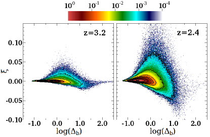
Figure 27: Hydrodynamical response of the gas to He ii reionization. Joint distribution of the gas overdensity ($\Delta_{\rm b}$) and the relative change of the local gas density between the T2 and T1 simulations ($\xi$). The color scale indicates the gas mass in each pixel (normalized to unity at maximum). Contour levels correspond to $0.1$, $1$, $5$, $10$, $15$, $30$, $50$ and $90$ per cent of the maximum value.

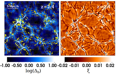
Figure 28: Left: density distribution in a slice of the T2 simulation. The transverse size is of $25\,\textrm{$h^{-1}\textrm{Mpc}$}$ and the yellow arrows indicate the velocity difference between cells in the T2 and in the T1 simulations. Right: spatial distribution of the variable $\xi$ in the same slice.

Appendix B Number of spectral bins

	H i	He i	He ii
Minimum energy (ryd)	1	1.8088	4
Maximum energy (ryd)	1.8088	4	40
No. of spectral bins:
Run 1	5	5	10
Run 2	7	7	22
Run 3	10	10	30
Run 4	15	15	45
Run 5	20	20	60

Table 5: Number of spectral bins used to test the convergence of the radiative-transfer scheme.

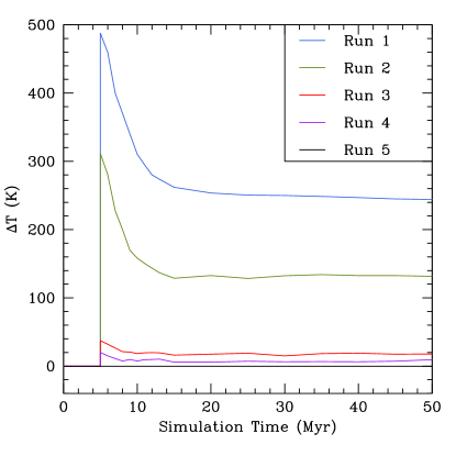
Figure 29: Influence of the frequency binning in the radiative-transfer scheme on to the temperature of a cell at mean density (see the main text for details). The variable $\Delta T$ indicates the difference between the actual temperature in a simulation and what is measured in the reference case, Run 5. Each curve corresponds to one of the simulations in Table 5 as indicated by the label.

RADAMESH samples the UV spectrum of the ionizing sources with a finite number of frequency bins which are logarithmically spaced. In order to optimize this choice, we perform a convergence study by considering a simulation box with a linear size of $25\,\textrm{$h^{-1}\textrm{Mpc}$}$. We start with a base grid of $64^{3}$ elements and add four levels of refinement during the evolution. The box is uniformly illuminated with a soft UV background generated by galaxies. At $z=3$, a single AGN (with a steady magnitude of $M_{1450}=-20.3$ and located at the centre of a massive dark matter halo) is turned on. We run a series of simulations by varying the binning strategy as detailed in Table 5. For each simulation, we follow the propagation of radiation for $50\,\textrm{Myr}$. To illustrate our results, we focus on a cell at mean density which is located $\simeq 1.1\,\textrm{$h^{-1}\textrm{Mpc}$}$ away from the active AGN.

In Fig. 29, we show the evolution of the temperature difference between each run and Run 5 which uses the largest number of spectral bins. Using too few bins overestimates the temperature of the gas, especially during the passage of the ionization front. For the number of spectral bins adopted in this work, the temperature increment with respect to the reference case is negligible.

Finally, it is interesting to quantify the impact of soft X-rays with energies above $40\,\textrm{ryd}$ that have been neglected in our study. For this reason, we run an additional simulation in which we extend the maximum photon energy to $80\,\textrm{ryd}$ and partition the He ii ionizing photons into 60 spectral bins. The extra heating caused by the energetic photons produces an early temperature increment of $\approx 150\,\textrm{K}$ (due to their long mean free path) which reduces to less than $50\,\textrm{K}$ a few Myr after the passage of the ionization front. We conclude that considering only photons with energies below $40\,\textrm{ryd}$ does not affect our results.

Appendix C Comparison between PLE and PDE source models

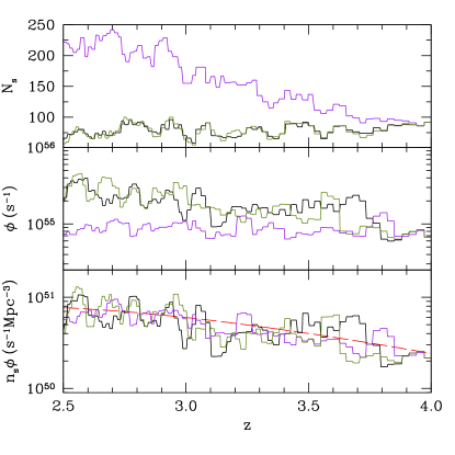
Figure 30: Comparison between different AGN models used in the L1 (green), L1b (black) and L2 (purple) simulations. Top: number of active sources. Centre: mean number of H i ionizing photons emitted by a single source per unit time. Bottom: total number of ionizing photons emitted per unit time and volume. The red dashed line shows the model predictions by Haardt & Madau (2012) that we use to calibrate the time evolution of the AGN emissivity.

As discussed in Section 2.3, we model the redshift evolution of the AGN emissivity either by modifying the number density of the sources (PDE model) or by altering their luminosity (PLE model). For illustrative purposes and to facilitate understanding, we show in Fig. 30 how the number of active sources (top panel), the mean number of ionizing photons (with energy above $1\,\textrm{ryd}$) emitted by a single source per unit time (middle panel) and the total emissivity of ionizing photons per unit time and volume (bottom panel) evolve in the L1, L1b and L2 simulations.

References

- Becker et al. (2011) Becker, G. D., Bolton, J. S., Haehnelt, M. G., & Sargent, W. L. W. 2011, MNRAS, 410, 1096
- Becker et al. (2012) Becker, G. D., Hewett, P. C., Worseck, G., & Prochaska, J. X. 2012, arXiv:1208.2584
- Bernardi et al. (2003) Bernardi, M., Sheth, R. K., SubbaRao, M., et al. 2003, AJ, 125, 32
- Bertschinger (2001) Bertschinger, E. 2001, ApJS, 137, 1
- Bolton et al. (2008) Bolton, J. S., Viel, M., Kim, T.-S., Haehnelt, M. G., & Carswell, R. F. 2008, MNRAS, 386, 1131
- Bolton et al. (2009a) Bolton, J. S., Oh, S. P., & Furlanetto, S. R. 2009a, MNRAS, 395, 736
- Bolton et al. (2009b) Bolton, J. S., Oh, S. P., & Furlanetto, S. R. 2009b, MNRAS, 396, 2405
- Bolton et al. (2012) Bolton, J. S., Becker, G. D., Raskutti, S., et al. 2012, MNRAS, 419, 2880
- Bryan & Machacek (2000) Bryan, G. L., & Machacek, M. E. 2000, ApJ, 534, 57
- Calura et al. (2012) Calura, F., Tescari, E., D’Odorico, V., et al. 2012, MNRAS, 422, 3019
- Cantalupo et al. (2007) Cantalupo, S., Lilly, S. J., & Porciani, C. 2007, ApJ, 657, 135
- Cantalupo & Porciani (2011) Cantalupo, S., & Porciani, C. 2011, MNRAS, 411, 1678
- Croft et al. (2002) Croft, R. A. C., Weinberg, D. H., Bolte, M., et al. 2002, ApJ, 581, 20
- Dall’Aglio et al. (2008) Dall’Aglio, A., Wisotzki, L., & Worseck, G. 2008, A&A, 491, 465
- Dall’Aglio et al. (2009) Dall’Aglio, A., Wisotzki, L., & Worseck, G. 2009, arXiv:0906.1484
- Davidsen et al. (1996) Davidsen, A. F., Kriss, G. A., & Zheng, W. 1996, Nature, 380, 47
- Eisenstein & Hut (1998) Eisenstein, D. J., & Hut, P. 1998, ApJ, 498, 137
- Fan et al. (2006a) Fan, X., Carilli, C. L., & Keating, B. 2006a, ARA&A, 44, 415
- Fan et al. (2006b) Fan, X., Strauss, M. A., Becker, R. H., et al. 2006b, AJ, 132, 117
- Fanidakis et al. (2013) Fanidakis, N., Maccio, A. V., Baugh, C. M., Lacey, C. G., & Frenk, C. S. 2013, arXiv:1305.2199
- Faucher-Giguère et al. (2008) Faucher-Giguère, C.-A., Prochaska, J. X., Lidz, A., Hernquist, L., & Zaldarriaga, M. 2008, ApJ, 681, 831
- Fechner et al. (2006) Fechner, C., Reimers, D., Kriss, G. A., et al. 2006, A&A, 455, 91
- Garzilli et al. (2012) Garzilli, A., Bolton, J. S., Kim, T.-S., Leach, S., & Viel, M. 2012, MNRAS, 424, 1723
- Glikman et al. (2011) Glikman, E., Djorgovski, S. G., Stern, D., et al. 2011, ApJL, 728, L26
- Haardt & Madau (2012) Haardt, F., & Madau, P. 2012, ApJ, 746, 125
- Haiman & Hui (2001) Haiman, Z., & Hui, L. 2001, ApJ, 547, 27
- Hogan et al. (1997) Hogan, C. J., Anderson, S. F., & Rugers, M. H. 1997, AJ, 113, 1495
- Hui & Gnedin (1997) Hui, L., & Gnedin, N. Y. 1997, MNRAS, 292, 27
- Jakobsen et al. (1994) Jakobsen, P., Boksenberg, A., Deharveng, J. M., et al. 1994, Nature, 370, 35
- Jakobsen et al. (2003) Jakobsen, P., Jansen, R. A., Wagner, S., & Reimers, D. 2003, A&A, 397, 891
- Jarosik et al. (2011) Jarosik, N., Bennett, C. L., Dunkley, J., et al. 2011, ApJS, 192, 14
- Jenkins et al. (2001) Jenkins, A., Frenk, C. S., White, S. D. M., et al. 2001, MNRAS, 321, 372
- Kim et al. (2007) Kim, T.-S., Bolton, J. S., Viel, M., Haehnelt, M. G., & Carswell, R. F. 2007, MNRAS, 382, 1657
- Komatsu et al. (2011) Komatsu, E., Smith, K. M., Dunkley, J., et al. 2011, ApJS, 192, 18
- Lidz et al. (2010) Lidz, A., Faucher-Giguère, C.-A., Dall’Aglio, A., et al. 2010, ApJ, 718, 199