A Scalable Approximate Model Counter

Abstract

Propositional model counting ($\#\mathsf{SAT}$), i.e., counting the number of satisfying assignments of a propositional formula, is a problem of significant theoretical and practical interest. Due to the inherent complexity of the problem, approximate model counting, which counts the number of satisfying assignments to within given tolerance and confidence level, was proposed as a practical alternative to exact model counting. Yet, approximate model counting has been studied essentially only theoretically. The only reported implementation of approximate model counting, due to Karp and Luby, worked only for DNF formulas. A few existing tools for CNF formulas are bounding model counters; they can handle realistic problem sizes, but fall short of providing counts within given tolerance and confidence, and, thus, are not approximate model counters.

We present here a novel algorithm, as well as a reference implementation, that is the first scalable approximate model counter for CNF formulas. The algorithm works by issuing a polynomial number of calls to a SAT solver. Our tool, $\mathsf{ApproxMC}$, scales to formulas with tens of thousands of variables. Careful experimental comparisons show that $\mathsf{ApproxMC}$ reports, with high confidence, bounds that are close to the exact count, and also succeeds in reporting bounds with small tolerance and high confidence in cases that are too large for computing exact model counts.

1 Introduction

Propositional model counting, also known as $\#\mathsf{SAT}$, concerns counting the number of models (satisfying truth assignments) of a given propositional formula. This problem has been the subject of extensive theoretical investigation since its introduction by Valiant [35] in 1979. Several interesting applications of $\#\mathsf{SAT}$ have been studied in the context of probabilistic reasoning, planning, combinatorial design and other related fields [24, 4, 9]. In particular, probabilistic reasoning and inferencing have attracted considerable interest in recent years [12], and stand to benefit significantly from efficient propositional model counters.

Theoretical investigations of $\#\mathsf{SAT}$ have led to the discovery of deep connections in complexity theory [3, 29, 33]: $\#\mathsf{SAT}$ is $\#\mathsf{P}$-complete, where $\#\mathsf{P}$ is the set of counting problems associated with decision problems in the complexity class $\mathsf{NP}$. Furthermore, $\mathsf{P}^{\#\mathsf{SAT}}$, that is, a polynomial-time machine with a $\#\mathsf{SAT}$ oracle, can solve all problems in the entire polynomial hierarchy. In fact, the polynomial-time machine only needs to make one $\#\mathsf{SAT}$ query to solve any problem in the polynomial hierarchy. This is strong evidence for the hardness of $\#\mathsf{SAT}$.

In many applications of model counting, such as in probabilistic reasoning, the exact model count may not be critically important, and approximate counts are sufficient. Even when exact model counts are important, the inherent complexity of the problem may force one to work with approximate counters in practice. In [31], Stockmeyer showed that counting models within a specified tolerance factor can be achieved in deterministic polynomial time using a $\Sigma_{2}^{p}$-oracle. Karp and Luby presented a fully polynomial randomized approximation scheme for counting models of a DNF formula [18]. Building on Stockmeyer’s result, Jerrum, Valiant and Vazirani [16] showed that counting models of CNF formulas within a specified tolerance factor can be solved in random polynomial time using an oracle for $\mathsf{SAT}$.

On the implementation front, the earliest approaches to $\#\mathsf{SAT}$ were based on DPLL-style $\mathsf{SAT}$ solvers and computed exact counts. These approaches consisted of incrementally counting the number of solutions by adding appropriate multiplication factors after a partial solution was found. This idea was formalized by Birnbaum and Lozinkii [6] in their model counter $\mathsf{CDP}$. Subsequent model counters such as $\mathsf{Relsat}$ [17], $\mathsf{Cachet}$ [26] and $\mathsf{sharpSAT}$ [32] improved upon this idea by using several optimizations such as component caching, clause learning, look-ahead and the like. Techniques based on Boolean Decision Diagrams and their variants [23, 21], or d-DNNF formulae [8], have also been used to compute exact model counts. Although exact model counters have been successfully used in small- to medium-sized problems, scaling to larger problem instances has posed significant challenges in practice. Consequently, a large class of practical applications has remained beyond the reach of exact model counters.

To counter the scalability challenge, more efficient techniques for counting models approximately have been proposed. These counters can be broadly divided into three categories. Counters in the first category are called $(\varepsilon,\delta)$ counters, following Karp and Luby’s terminology [18]. Let $\varepsilon$ and $\delta$ be real numbers such that $0<\varepsilon\leq 1$ and $0<\delta\leq 1$. For every propositional formula $F$ with $\#F$ models, an $(\varepsilon,\delta)$ counter computes a number that lies in the interval $[(1+\varepsilon)^{-1}\#F,(1+\varepsilon)\#F]$ with probability at least $1-\delta$. We say that $\varepsilon$ is the tolerance of the count, and $1-\delta$ is its confidence. The counter described in this paper and also that due to Karp and Luby [18] belong to this category. The approximate-counting algorithm of Jerrum et al. [16] also belongs to this category; however, their algorithm does not lend itself to an implementation that scales in practice. Counters in the second category are called lower (or upper) bounding counters, and are parameterized by a confidence probability $1-\delta$. For every propositional formula $F$ with $\#F$ models, an upper (resp., lower) bounding counter computes a number that is at least as large (resp., as small) as $\#F$ with probability at least $1-\delta$. Note that bounding counters do not provide any tolerance guarantees. The large majority of approximate counters used in practice are bounding counters. Notable examples include $\mathsf{SampleCount}$ [14], $\mathsf{BPCount}$ [20], $\mathsf{MBound}$ (and $\mathsf{Hybrid}$-$\mathsf{MBound}$) [13], and $\mathsf{MiniCount}$ [20]. The final category of counters is called guarantee-less counters. These counters provide no guarantees at all but they can be very efficient and provide good approximations in practice. Examples of guarantee-less counters include $\mathsf{ApproxCount}$ [36], $\mathsf{SearchTreeSampler}$ [10], $\mathsf{SE}$ [25] and $\mathsf{SampleSearch}$ [11].

Bounding both the tolerance and confidence of approximate model counts is extremely valuable in applications like probabilistic inference. Thus, designing $(\varepsilon,\delta)$ counters that scale to practical problem sizes is an important problem. Earlier work on $(\varepsilon,\delta)$ counters has been restricted largely to theoretical treatments of the problem. The only counter in this category that we are aware of as having been implemented is due to Karp and Luby [22]. Karp and Luby’s original implementation was designed to estimate reliabilities of networks with failure-prone links. However, the underlying Monte Carlo engine can be used to approximately count models of DNF, but not CNF, formulas.

The counting problems for both CNF and DNF formulae are $\#\mathsf{P}$-complete. While the DNF representation suits some applications, most modern applications of model counting (e.g. probabilistic inference) use the CNF representation. Although exact counting for DNF and CNF formulae are polynomially inter-reducible, there is no known polynomial reduction for the corresponding approximate counting problems. In fact, Karp and Luby remark in [18] that it is highly unlikely that their randomized approximate algorithm for DNF formulae can be adapted to work for CNF formulae. Thus, there has been no prior implementation of $(\varepsilon,\delta)$ counters for CNF formulae that scales in practice. In this paper, we present the first such counter. As in [16], our algorithm runs in random polynomial time using an oracle for $\mathsf{SAT}$. Our extensive experiments show that our algorithm scales, with low error, to formulae arising from several application domains involving tens of thousands of variables.

The organization of the paper is as follows. We present preliminary material in Section 2, and related work in Section 3. In Section 4, we present our algorithm, followed by its analysis in Section 5. Section 6 discusses our experimental methodology, followed by experimental results in Section 7. Finally, we conclude in Section 8.

2 Notation and Preliminaries

Let $\Sigma$ be an alphabet and $R\subseteq\Sigma^{*}\times\Sigma^{*}$ be a binary relation. We say that $R$ is an $\mathcal{NP}$-relation if $R$ is polynomial-time decidable, and if there exists a polynomial $p(\cdot)$ such that for every $(x,y)\in R$, we have $|y|\leq p(|x|)$. Let $L_{R}$ be the language $\{x\in\Sigma^{*}\mid\exists y\in\Sigma^{*},\,(x,y)\in R\}$. The language $L_{R}$ is said to be in $\mathcal{NP}$ if $R$ is an $\mathcal{NP}$-relation. The set of all satisfiable propositional logic formulae in CNF is a language in $\mathcal{NP}$. Given $x\in L_{R}$, a witness or model of $x$ is a string $y\in\Sigma^{*}$ such that $(x,y)\in R$. The set of all models of $x$ is denoted $R_{x}$. For notational convenience, fix $\Sigma$ to be $\{0,1\}$ without loss of generality. If $R$ is an $\mathcal{NP}$-relation, we may further assume that for every $x\in L_{R}$, every witness $y\in R_{x}$ is in $\{0,1\}^{n}$, where $n=p(|x|)$ for some polynomial $p(\cdot)$.

Let $R\subseteq\{0,1\}^{*}\times\{0,1\}^{*}$ be an $\mathcal{NP}$ relation. The counting problem corresponding to $R$ asks “Given $x\in\{0,1\}^{*}$, what is $|R_{x}|$?”. If $R$ relates CNF propositional formulae to their satisfying assignments, the corresponding counting problem is called $\#\mathsf{SAT}$. The primary focus of this paper is on $(\varepsilon,\delta)$ counters for $\#\mathsf{SAT}$. The randomized $(\varepsilon,\delta)$ counters of Karp and Luby [18] for DNF formulas are fully polynomial, which means that they run in time polynomial in the size of the input formula $F$, $1/\varepsilon$ and $\log(1/\delta)$. The randomized $(\varepsilon,\delta)$ counters for CNF formulas in [16] and in this paper are however fully polynomial with respect to a SAT oracle.

A special class of hash functions, called $r$-wise independent hash functions, play a crucial role in our work. Let $n,m$ and $r$ be positive integers, and let $H(n,m,r)$ denote a family of $r$-wise independent hash functions mapping $\{0,1\}^{n}$ to $\{0,1\}^{m}$. We use $\mathsf{Pr}\left[X:{\cal P}\right]$ to denote the probability of outcome $X$ when sampling from a probability space ${\cal P}$, and $h\xleftarrow{R}H(n,m,r)$ to denote the probability space obtained by choosing a hash function $h$ uniformly at random from $H(n,m,r)$. The property of $r$-wise independence guarantees that for all $\alpha_{1},\ldots\alpha_{r}\in\{0,1\}^{m}$ and for all distinct $y_{1},\ldots y_{r}\in\{0,1\}^{n}$, $\mathsf{Pr}\left[\bigwedge_{i=1}^{r}h(y_{i})=\alpha_{i}\right.$ $\left.:h\xleftarrow{R}H(n,m,r)\right]=2^{-mr}$. For every $\alpha\in\{0,1\}^{m}$ and $h\in H(n,m,r)$, let $h^{-1}(\alpha)$ denote the set $\{y\in\{0,1\}^{n}\mid h(y)=\alpha\}$. Given $R_{x}\subseteq\{0,1\}^{n}$ and $h\in H(n,m,r)$, we use $R_{x,h,\alpha}$ to denote the set $R_{x}\cap h^{-1}(\alpha)$. If we keep $h$ fixed and let $\alpha$ range over $\{0,1\}^{m}$, the sets $R_{x,h,\alpha}$ form a partition of $R_{x}$. Following the notation in  [5], we call each element of such a partition a cell of $R_{x}$ induced by $h$. It was shown in [5] that if $h$ is chosen uniformly at random from $H(n,m,r)$ for $r\geq 1$, then the expected size of $R_{x,h,\alpha}$, denoted $\mathsf{E}\left[|R_{x,h,\alpha}|\right]$, is $|R_{x}|/2^{m}$, for each $\alpha\in\{0,1\}^{m}$.

The specific family of hash functions used in our work, denoted $H_{xor}(n,m,3)$, is based on randomly choosing bits from $y\in\{0,1\}^{n}$ and xor-ing them. This family of hash functions has been used in earlier work  [13], and has been shown to be 3-independent in  [15]. Let $h(y)[i]$ denote the $i^{th}$ component of the bit-vector obtained by applying hash function $h$ to $y$. The family $H_{xor}(n,m,3)$ is defined as $\{h(y)\mid(h(y))[i]=a_{i,0}\oplus(\bigoplus_{k=1}^{n}a_{i,k}\cdot y[k]),a_{i,j}\in\{0,1\},1\leq i\leq m,0\leq j\leq n\}$, where $\oplus$ denotes the xor operation. By randomly choosing the $a_{i,j}$’s, we can randomly choose a hash function from this family.

3 Related Work

Sipser pioneered a hashing based approach in  [30], which has subsequently been used in theoretical  [34, 5] and practical  [15, 13, 7] treatments of approximate counting and (near-)uniform sampling. Earlier implementations of counters that use the hashing-based approach are $\mathsf{MBound}$ and $\mathsf{Hybrid}$-$\mathsf{MBound}$ [13]. Both these counters use the same family of hashing functions, i.e., $H_{xor}(n,m,3)$, that we use. Nevertheless, there are significant differences between our algorithm and those of $\mathsf{MBound}$ and $\mathsf{Hybrid}$-$\mathsf{MBound}$. Specifically, we are able to exploit properties of the $H_{xor}(n,m,3)$ family of hash functions to obtain a fully polynomial $(\varepsilon,\delta)$ counter with respect to a SAT oracle. In contrast, both $\mathsf{MBound}$ and $\mathsf{Hybrid}$-$\mathsf{MBound}$ are bounding counters, and cannot provide bounds on tolerance. In addition, our algorithm requires no additional parameters beyond the tolerance $\varepsilon$ and confidence $1-\delta$. In contrast, the performance and quality of results of both $\mathsf{MBound}$ and $\mathsf{Hybrid}$-$\mathsf{MBound}$, depend crucially on some hard-to-estimate parameters. It has been our experience that the right choice of these parameters is often domain dependent and difficult.

Jerrum, Valiant and Vazirani [16] showed that if $R$ is a self-reducible $\mathcal{NP}$ relation (such as SAT), the problem of generating models almost uniformly is polynomially inter-reducible with approximately counting models. The notion of almost uniform generation requires that if $x$ is a problem instance, then for every $y\in R_{x}$, we have $(1+\varepsilon)^{-1}\varphi(x)$ $\leq$ $\mathsf{Pr}[y\mbox{ is generated}]$ $\leq$ $(1+\varepsilon)\varphi(x)$, where $\varepsilon>0$ is the specified tolerance and $\varphi(x)$ is an appropriate function. Given an almost uniform generator $\mathcal{G}$ for $R$, an input $x$, a tolerance bound $\varepsilon$ and an error probability bound $\delta$, it is shown in [16] that one can obtain an $(\varepsilon,\delta)$ counter for $R$ by invoking $\mathcal{G}$ polynomially (in $|x|$, $1/\varepsilon$ and $\log_{2}(1/\delta)$) many times, and by using the generated samples to estimate $|R_{x}|$. For convenience of exposition, we refer to this approximate-counting algorithm as the $\mathsf{JVV}$ algorithm (after the last names of the authors).

An important feature of the $\mathsf{JVV}$ algorithm is that it uses the almost uniform generator $\mathcal{G}$ as a black box. Specifically, the details of how $\mathcal{G}$ works is of no consequence. Prima facie, this gives us freedom in the choice of $\mathcal{G}$ when implementing the $\mathsf{JVV}$ algorithm. Unfortunately, while there are theoretical constructions of uniform generators in [5], we are not aware of any implementation of an almost uniform generator that scales to CNF formulas involving thousands of variables. The lack of a scalable and almost uniform generator presents a significant hurdle in implementing the $\mathsf{JVV}$ algorithm for practical applications. It is worth asking if we can make the $\mathsf{JVV}$ algorithm work without requiring $\mathcal{G}$ to be an almost uniform generator. A closer look at the proof of correctness of the $\mathsf{JVV}$ algorithm [16] shows it relies crucially on the ability of $\mathcal{G}$ to ensure that the probabilities of generation of any two distinct models of $x$ differ by a factor in $O(\varepsilon^{2})$. As discussed in [7], existing algorithms for randomly generating models either provide this guarantee but scale very poorly in practice (e.g., the algorithms in [5, 37]), or scale well in practice without providing the above guarantee (e.g., the algorithms in [7, 15, 19]). Therefore, using an existing generator as a black box in the $\mathsf{JVV}$ algorithm would not give us an $(\varepsilon,\delta)$ model counter that scales in practice. The primary contribution of this paper is to show that a scalable $(\varepsilon,\delta)$ counter can indeed be designed by using the same insights that went into the design of a near uniform generator, $\mathsf{UniWit}$ [7], but without using the generator as a black box in the approximate counting algorithm. Note that near uniformity, as defined in [7], is an even more relaxed notion of uniformity than almost uniformity. We leave the question of whether a near uniform generator can be used as a black box to design an $(\varepsilon,\delta)$ counter as part of future work.

The central idea of $\mathsf{UniWit}$, which is also shared by our approximate model counter, is the use of $r$-wise independent hashing functions to randomly partition the space of all models of a given problem instance into “small” cells. This idea was first proposed in [5], but there are two novel insights that allow $\mathsf{UniWit}$ [7] to scale better than other hashing-based sampling algorithms [5, 15], while still providing guarantess on the quality of sampling. These insights are: (i) the use of computationally efficient linear hashing functions with low degrees of independence, and (ii) a drastic reduction in the size of “small” cells, from $n^{2}$ in [5] to $n^{1/k}$ (for $2\leq k\leq 3$) in [7], and even further to a constant in the current paper. We continue to use these key insights in the design of our approximate model counter, although $\mathsf{UniWit}$ is not used explicitly in the model counter.

4 Algorithm

We now describe our approximate model counting algorithm, called $\mathsf{ApproxMC}$. As mentioned above, we use $3$-wise independent linear hashing functions from the $H_{xor}(n,m,3)$ family, for an appropriate $m$, to randomly partition the set of models of an input formula into “small” cells. In order to test whether the generated cells are indeed small, we choose a random cell and check if it is non-empty and has no more than $pivot$ elements, where $pivot$ is a threshold that depends only on the tolerance bound $\varepsilon$. If the chosen cell is not small, we randomly partition the set of models into twice as many cells as before by choosing a random hashing function from the family $H_{xor}(n,m+1,3)$. The above procedure is repeated until either a randomly chosen cell is found to be non-empty and small, or the number of cells exceeds $\frac{2^{n+1}}{\mathit{pivot}}$. If all cells that were randomly chosen during the above process were either empty or not small, we report a counting failure and return $\bot$. Otherwise, the size of the cell last chosen is scaled by the number of cells to obtain an $\varepsilon$-approximate estimate of the model count.

The procedure outlined above forms the core engine of $\mathsf{ApproxMC}$. For convenience of exposition, we implement this core engine as a function $\mathsf{ApproxMCCore}$. The overall $\mathsf{ApproxMC}$ algorithm simply invokes $\mathsf{ApproxMCCore}$ sufficiently many times, and returns the median of the non-$\bot$ values returned by $\mathsf{ApproxMCCore}$. The pseudocode for algorithm $\mathsf{ApproxMC}$ is shown below.

Algorithm ${\mathsf{ApproxMC}}(F,\varepsilon,\delta)$ 1: $\mathit{counter}\leftarrow 0;C\leftarrow\mathsf{emptyList}$; 2: $\mathit{pivot}\leftarrow 2\times{\mathsf{ComputeThreshold}}(\varepsilon)$; 3: $t\leftarrow{\mathsf{ComputeIterCount}}(\delta)$; 4: repeat: 5: $c\leftarrow{\mathsf{ApproxMCCore}}(F,\mathit{pivot})$; 6: $\mathit{counter}\leftarrow\mathit{counter}+1$; 7: if $(c\neq\bot)$ 8: $\mathsf{AddToList}(C,c)$; 9: until ($\mathit{counter}<t$); 10: $\mathit{finalCount}\leftarrow\mathsf{FindMedian}(C)$; 11: return $\mathit{finalCount}$;

Algorithm ${\mathsf{ComputeThreshold}}(\varepsilon)$ 1: return $\left\lceil 3e^{1/2}\left(1+\frac{1}{\varepsilon}\right)^{2}\right\rceil$; Algorithm ${\mathsf{ComputeIterCount}}(\delta)$ 1: return $\left\lceil 35\log_{2}(3/\delta)\right\rceil$;

Algorithm $\mathsf{ApproxMC}$ takes as inputs a CNF formula $F$, a tolerance $\varepsilon~{}(0<\varepsilon\leq 1)$ and $\delta~{}(0<\delta\leq 1)$ such that the desired confidence is $1-\delta$. It computes two key parameters: (i) a threshold $\mathit{pivot}$ that depends only on $\varepsilon$ and is used in $\mathsf{ApproxMCCore}$ to determine the size of a “small” cell, and (ii) a parameter $t~{}(\geq 1)$ that depends only on $\delta$ and is used to determine the number of times $\mathsf{ApproxMCCore}$ is invoked. The particular choice of functions to compute the parameters $\mathit{pivot}$ and $t$ aids us in proving theoretical guarantees for $\mathsf{ApproxMC}$ in Section 5. Note that $\mathit{pivot}$ is in $\mathcal{O}(1/\varepsilon^{2})$ and $t$ is in $\mathcal{O}(\log_{2}(1/\delta))$. All non-$\bot$ estimates of the model count returned by $\mathsf{ApproxMCCore}$ are stored in the list $C$. The function $\mathsf{AddToList}(C,c)$ updates the list $C$ by adding the element $c$. The final estimate of the model count returned by $\mathsf{ApproxMC}$ is the median of the estimates stored in $C$, computed using $\mathsf{FindMedian}(C)$. We assume that if the list $C$ is empty, $\mathsf{FindMedian}(C)$ returns $\bot$.

The pseudocode for algorithm $\mathsf{ApproxMCCore}$ is shown below.

Algorithm ${\mathsf{ApproxMCCore}}(F,pivot)$
/* Assume $z_{1},\ldots z_{n}$ are the variables of $F$ */
1:	$S\leftarrow\mathsf{BoundedSAT}(F,\mathit{pivot}+1)$;
2:	if ($|S|\leq\mathit{pivot}$)
3:		return $|S|$;
4:	else
5:		$l\leftarrow\lfloor\log_{2}(\mathit{pivot})\rfloor-1$; $i\leftarrow l-1$;
6:		repeat
7:			$i\leftarrow i+1$;
8:			Choose $h$ at random from $H_{xor}(n,i-l,3)$;
9:			Choose $\alpha$ at random from $\{0,1\}^{i-l}$;
10:			$S\leftarrow\mathsf{BoundedSAT}(F\wedge(h(z_{1},\ldots z_{n})=\alpha),\mathit{pivot}+1)$;
11:		until ($1\leq|S|\leq\mathit{pivot}$) or ($i=n$);
12:		if ($|S|>\mathit{pivot}$ or $|S|=0$) return $\bot$ ;
13:		else return $|S|\cdot 2^{i-l}$;

Algorithm $\mathsf{ApproxMCCore}$ takes as inputs a CNF formula $F$ and a threshold $pivot$, and returns an $\varepsilon$-approximate estimate of the model count of $F$. We assume that $\mathsf{ApproxMCCore}$ has access to a function $\mathsf{BoundedSAT}$ that takes as inputs a proposition formula $F^{\prime}$ that is the conjunction of a CNF formula and xor constraints, as well as a threshold $v\geq 0$. $\mathsf{BoundedSAT}$$(F^{\prime},v)$ returns a set $S$ of models of $F^{\prime}$ such that $|S|=\min(v,\#F^{\prime})$. If the model count of $F$ is no larger than $\mathit{pivot}$, then $\mathsf{ApproxMCCore}$ returns the exact model count of $F$ in line $3$ of the pseudocode. Otherwise, it partitions the space of all models of $F$ using random hashing functions from $H_{xor}(n,i-l,3)$ and checks if a randomly chosen cell is non-empty and has at most $\mathit{pivot}$ elements. Lines $8$–$10$ of the repeat-until loop in the pseudocode implement this functionality. The loop terminates if either a randomly chosen cell is found to be small and non-empty, or if the number of cells generated exceeds $\frac{2^{n+1}}{\mathit{pivot}}$ (if $i=n$ in line $11$, the number of cells generated is $2^{n-l}\geq\frac{2^{n+1}}{\mathit{pivot}}$). In all cases, unless the cell that was chosen last is empty or not small, we scale its size by the number of cells generated by the corresponding hashing function to compute an estimate of the model count. If, however, all randomly chosen cells turn out to be empty or not small, we report a counting error by returning $\bot$.

Implementation issues: There are two steps in algorithm $\mathsf{ApproxMCCore}$ (lines 8 and 9 of the pseudocode) where random choices are made. Recall from Section 2 that choosing a random hash function from $H_{xor}(n,m,3)$ requires choosing random bit-vectors. It is straightforward to implement these choices and also the choice of a random $\alpha\in\{0,1\}^{i-l}$ in line 9 of the pseudocode, if we have access to a source of independent and uniformly distributed random bits. Our implementation uses pseudo-random sequences of bits generated from nuclear decay processes and made available at HotBits [2]. We download and store a sufficiently long sequence of random bits in a file, and access an appropriate number of bits sequentially whenever needed. We defer experimenting with sequences of bits obtained from other pseudo-random generators to a future study.

In lines 1 and 10 of the pseudocode for algorithm $\mathsf{ApproxMCCore}$, we invoke the function $\mathsf{BoundedSAT}$. Note that if $h$ is chosen randomly from $H_{xor}(n,m,3)$, the formula for which we seek models is the conjunction of the original (CNF) formula and xor constraints encoding the inclusion of each witness in $h^{-1}(\alpha)$. We therefore use a SAT solver optimized for conjunctions of xor constraints and CNF clauses as the back-end engine. Specifically, we use CryptoMiniSAT (version 2.9.2) [1], which also allows passing a parameter indicating the maximum number of witnesses to be generated.

Recall that $\mathsf{ApproxMCCore}$ is invoked $t$ times with the same arguments in algorithm $\mathsf{ApproxMC}$. Repeating the loop of lines 6–11 in the pseudocode of $\mathsf{ApproxMCCore}$ in each invocation can be time consuming if the values of $i-l$ for which the loop terminates are large. In [7], a heuristic called leap-frogging was proposed to overcome this bottleneck in practice. With leap-frogging, we register the smallest value of $i-l$ for which the loop terminates during the first few invocations of $\mathsf{ApproxMCCore}$. In all subsequent invocations of $\mathsf{ApproxMCCore}$ with the same arguments, we start iterating the loop of lines 6–11 by initializing $i-l$ to the smallest value registered from earlier invocations. Our experiments indicate that leap-frogging is extremely efficient in practice and leads to significant savings in time after the first few invocations of $\mathsf{ApproxMCCore}$. A theoretical analysis of leapfrogging is deferred to future work.

5 Analysis of $\mathsf{ApproxMC}$

The following result, a minor variation of Theorem 5 in [28], about Chernoff-Hoeffding bounds plays an important role in our analysis.

Theorem 5.1

Let $\Gamma$ be the sum of $r$-wise independent random variables, each of which is confined to the interval $[0,1]$, and suppose $\mathsf{E}[\Gamma]=\mu$. For $0<\beta\leq 1$, if $r\leq\left\lfloor\beta^{2}\mu e^{-1/2}\right\rfloor\leq 4$ , then $\mathsf{Pr}\left[\,|\Gamma-\mu|\geq\beta\mu\,\right]\leq e^{-r/2}$.

Let $F$ be a CNF propositional formula with $n$ variables. The next two lemmas show that algorithm $\mathsf{ApproxMCCore}$, when invoked from $\mathsf{ApproxMC}$ with arguments $F$, $\varepsilon$ and $\delta$, behaves like an $(\varepsilon,d)$ model counter for $F$, for a fixed confidence $1-d$ (possibly different from $1-\delta$). Throughout this section, we use the notations $R_{F}$ and $R_{F,h,\alpha}$ introduced in Section 2.

Lemma 1

Let algorithm $\mathsf{ApproxMCCore}$, when invoked from $\mathsf{ApproxMC}$, return $c$ with $i$ being the final value of the loop counter in $\mathsf{ApproxMCCore}$. Then, $\mathsf{Pr}\left[(1+\varepsilon)^{-1}\cdot|R_{F}|\leq c\leq(1+\varepsilon)\cdot|R_{F}|\Bigm{|}c\neq\bot\mbox{ and }i\leq\log_{2}|R_{F}|\right]$ $\geq 1-e^{-3/2}$.

Proof

Referring to the pseudocode of $\mathsf{ApproxMCCore}$, the lemma is trivially satisfied if $|R_{F}|\leq\mathit{pivot}$. Therefore, the only non-trivial case to consider is when $|R_{F}|>\mathit{pivot}$ and $\mathsf{ApproxMCCore}$ returns from line $13$ of the pseudocode. In this case, the count returned is $2^{i-l}.|R_{F,h,\alpha}|$, where $l=\lfloor\log_{2}(\mathit{pivot})\rfloor-1$ and $\alpha,i$ and $h$ denote (with abuse of notation) the values of the corresponding variables and hash functions in the final iteration of the repeat-until loop in lines $6$–$11$ of the pseudocode.

For simplicity of exposition, we assume henceforth that $\log_{2}(\mathit{pivot})$ is an integer. A more careful analysis removes this restriction with only a constant factor scaling of the probabilities. From the pseudocode of $\mathsf{ApproxMCCore}$, we know that $\mathit{pivot}=2\left\lceil 3e^{1/2}\left(1+\frac{1}{\varepsilon}\right)^{2}\right\rceil$.

Furthermore, the value of $i$ is always in $\{l,\ldots n\}$. Since $\mathit{pivot}<|R_{F}|\leq 2^{n}$ and $l=\lfloor\log_{2}\mathit{pivot}\rfloor-1$, we have $l<\log_{2}|R_{F}|\leq n$. The lemma is now proved by showing that for every $i$ in $\{l,\ldots\lfloor\log_{2}|R_{F}|\rfloor\}$, $h\in H(n,i-l,3)$ and $\alpha\in\{0,1\}^{i-l}$, we have $\mathsf{Pr}\left[(1+\varepsilon)^{-1}\cdot|R_{F}|\leq 2^{i-l}|R_{F,h,\alpha}|\right.$ $\left.\leq(1+\varepsilon)\cdot|R_{F}|\right]$ $\geq(1-e^{-3/2})$.

For every $y\in\{0,1\}^{n}$ and for every $\alpha\in\{0,1\}^{i-l}$, define an indicator variable $\gamma_{y,\alpha}$ as follows: $\gamma_{y,\alpha}=1$ if $h(y)=\alpha$, and $\gamma_{y,\alpha}=0$ otherwise. Let us fix $\alpha$ and $y$ and choose $h$ uniformly at random from $H(n,i-l,3)$. The random choice of $h$ induces a probability distribution on $\gamma_{y,\alpha}$, such that $\mathsf{Pr}\left[\gamma_{y,\alpha}=1\right]=\mathsf{Pr}\left[h(y)=\alpha\right]=2^{-(i-l)}$, and $\mathsf{E}\left[\gamma_{y,\alpha}\right]=\mathsf{Pr}\left[\gamma_{y,\alpha}=1\right]=2^{-(i-l)}$. In addition, the $3$-wise independence of hash functions chosen from $H(n,i-l,3)$ implies that for every distinct $y_{a},y_{b},y_{c}\in R_{F}$, the random variables $\gamma_{y_{a},\alpha}$, $\gamma_{y_{b},\alpha}$ and $\gamma_{y_{c},\alpha}$ are $3$-wise independent.

Let $\Gamma_{\alpha}=\sum_{y\in R_{F}}\gamma_{y,\alpha}$ and $\mu_{\alpha}=\mathsf{E}\left[\Gamma_{\alpha}\right]$. Clearly, $\Gamma_{\alpha}=|R_{F,h,\alpha}|$ and $\mu_{\alpha}=\sum_{y\in R_{F}}\mathsf{E}\left[\gamma_{y,\alpha}\right]=2^{-(i-l)}|R_{F}|$. Since $|R_{F}|>\mathit{pivot}$ and $i\leq\log_{2}|R_{F}|$, using the expression for $\mathit{pivot}$, we get $3\leq\left\lfloor e^{-1/2}(1+\frac{1}{\varepsilon})^{-2}\cdot\frac{|R_{F}|}{2^{i-l}}\right\rfloor$. Therefore, using Theorem 5.1, $\mathsf{Pr}\left[|R_{F}|.\left(1-\frac{\varepsilon}{1+\varepsilon}\right)\leq 2^{i-l}|R_{F,h,\alpha}|\right.$ $\left.\leq(1+\frac{\varepsilon}{1+\varepsilon})|R_{F}|\right]\geq 1-e^{-3/2}$. Simplifying and noting that $\frac{\varepsilon}{1+\varepsilon}<\varepsilon$ for all $\varepsilon>0$, we obtain $\mathsf{Pr}\left[(1+\varepsilon)^{-1}\cdot|R_{F}|\leq\right.$ $\left.2^{i-l}|R_{F,h,\alpha}|\leq(1+\varepsilon)\cdot|R_{F}|\right]\geq 1-e^{-3/2}$.

Lemma 2

Given $|R_{F}|>\mathit{pivot}$, the probability that an invocation of $\mathsf{ApproxMCCore}$ from $\mathsf{ApproxMC}$ returns non-$\bot$ with $i\leq\log_{2}|R_{F}|$, is at least $1-e^{-3/2}$.

Proof

Let us denote $\log_{2}|R_{F}|-l$ $=$ $\log_{2}|R_{F}|-(\left\lfloor\log_{2}(\mathit{pivot})\right\rfloor-1)$ by $m$. Since $|R_{F}|>\mathit{pivot}$ and $|R_{F}|\leq 2^{n}$, we have $l<m+l\leq n$. Let $p_{i}~{}(l\leq i\leq n)$ denote the conditional probability that $\mathsf{ApproxMCCore}$$(F,\mathit{pivot})$ terminates in iteration $i$ of the repeat-until loop (lines $6$–$11$ of the pseudocode) with $1\leq|R_{F,h,\alpha}|\leq\mathit{pivot}$, given $|R_{F}|>\mathit{pivot}$. Since the choice of $h$ and $\alpha$ in each iteration of the loop are independent of those in previous iterations, the conditional probability that $\mathsf{ApproxMCCore}$$(F,\mathit{pivot})$ returns non-$\bot$ with $i\leq\log_{2}|R_{F}|=m+l$, given $|R_{F}|>\mathit{pivot}$, is $p_{l}+(1-p_{l})p_{l+1}$ $+\cdots+(1-p_{l})(1-p_{l+1})\cdots(1-p_{m+l-1})p_{m+l}$. Let us denote this sum by $P$. Thus, $P=p_{l}+\sum_{i=l+1}^{m+l}\prod_{k=l}^{i-1}(1-p_{k})p_{i}$ $\,\geq\,\left(p_{l}+\sum_{i=l+1}^{m+l-1}\prod_{k=l}^{i-1}(1-p_{k})p_{i}\right)p_{m+l}$ $+$ $\prod_{s=l}^{m+l-1}(1-p_{s})p_{m+l}$ $=p_{m+l}$. The lemma is now proved by using Theorem 5.1 to show that $p_{m+l}\geq 1-e^{-3/2}$.

It was shown in Lemma 5.1 that $\mathsf{Pr}\left[(1+\varepsilon)^{-1}\cdot|R_{F}|\leq 2^{i-l}|R_{F,h,\alpha}|\right.$ $\left.\leq(1+\varepsilon)\cdot|R_{F}|\right]\geq 1-e^{-3/2}$ for every $i\in\{l,\ldots\lfloor\log_{2}|R_{F}|\rfloor\}$, $h\in H(n,i-l,3)$ and $\alpha\in\{0,1\}^{i-l}$. Substituting $\log_{2}|R_{F}|=m+l$ for $i$, re-arranging terms and noting that the definition of $m$ implies $2^{-m}|R_{F}|=\mathit{pivot}/2$, we get $\mathsf{Pr}\left[(1+\varepsilon)^{-1}(\mathit{pivot}/2)\right.$ $\left.\leq|R_{F,h,\alpha}|\right.$ $\left.\leq(1+\varepsilon)(\mathit{pivot}/2)\right]\geq 1-e^{-3/2}$. Since $0<\varepsilon\leq 1$ and $\mathit{pivot}>4$, it follows that $\mathsf{Pr}\left[1\leq|R_{F,h,\alpha}|\leq\mathit{pivot}\right]$ $\geq$ $1-e^{-3/2}$. Hence, $p_{m+l}\geq 1-e^{-3/2}$.

Theorem 5.2

Let an invocation of $\mathsf{ApproxMCCore}$ from $\mathsf{ApproxMC}$ return $c$. Then $\mathsf{Pr}\left[c\neq\bot\mbox{ and }(1+\varepsilon)^{-1}\cdot|R_{F}|\leq c\leq(1+\varepsilon)\cdot|R_{F}|\right]$ $\geq(1-e^{-3/2})^{2}>0.6$.

Proof sketch: It is easy to see that the required probability is at least as large as $\mathsf{Pr}\left[c\neq\bot\mbox{ and }i\leq\log_{2}|R_{F}|\mbox{ and }(1+\varepsilon)^{-1}\cdot|R_{F}|\leq c\leq(1+\varepsilon)\cdot|R_{F}|\right]$. From Lemmas 1 and 2, the latter probability is $\geq(1-e^{-3/2})^{2}$.

We now turn to proving that the confidence can be raised to at least $1-\delta$ for $\delta\in(0,1]$ by invoking $\mathsf{ApproxMCCore}$ $\mathcal{O}(\log_{2}(1/\delta))$ times, and by using the median of the non-$\bot$ counts thus returned. For convenience of exposition, we use $\eta(t,m,p)$ in the following discussion to denote the probability of at least $m$ heads in $t$ independent tosses of a biased coin with $\mathsf{Pr}\left[\mathit{heads}\right]=p$. Clearly, $\eta(t,m,p)=\sum_{k=m}^{t}\binom{t}{k}p^{k}(1-p)^{t-k}$.

Theorem 5.3

Given a propositional formula $F$ and parameters $\varepsilon~{}(0<\varepsilon\leq 1)$ and $\delta~{}(0<\delta\leq 1)$, suppose $\mathsf{ApproxMC}$$(F,\varepsilon,\delta)$ returns $c$. Then $\mathsf{Pr}\left[{\left(1+\varepsilon\right)}^{-1}\cdot|R_{F}|\leq c\right.$ $\left.\leq(1+\varepsilon)\cdot|R_{F}|\right]$ $\geq 1-\delta$.

Proof

Throughout this proof, we assume that $\mathsf{ApproxMCCore}$ is invoked $t$ times from $\mathsf{ApproxMC}$, where $t=\left\lceil 35\log_{2}(3/\delta)\right\rceil$ (see pseudocode for $\mathsf{ComputeIterCount}$ in Section 4). Referring to the pseudocode of $\mathsf{ApproxMC}$, the final count returned by $\mathsf{ApproxMC}$ is the median of non-$\bot$ counts obtained from the $t$ invocations of $\mathsf{ApproxMCCore}$. Let $Err$ denote the event that the median is not in $\left[(1+\varepsilon)^{-1}\cdot|R_{F}|,(1+\varepsilon)\cdot|R_{F}|\right]$. Let “$\#\mathit{non}\bot=q$” denote the event that $q$ (out of $t$) values returned by $\mathsf{ApproxMCCore}$ are non-$\bot$. Then, $\mathsf{Pr}\left[Err\right]$ $=$ $\sum_{q=0}^{t}\mathsf{Pr}\left[Err\mid\#\mathit{non}\bot=q\right]$ $\cdot$ $\mathsf{Pr}\left[\#\mathit{non}\bot=q\right]$.

In order to obtain $\mathsf{Pr}\left[Err\mid\#\mathit{non}\bot=q\right]$, we define a $0$-$1$ random variable $Z_{i}$, for $1\leq i\leq t$, as follows. If the $i^{th}$ invocation of $\mathsf{ApproxMCCore}$ returns $c$, and if $c$ is either $\bot$ or a non-$\bot$ value that does not lie in the interval $[(1+\varepsilon)^{-1}\cdot|R_{F}|,(1+\varepsilon)\cdot|R_{F}|]$, we set $Z_{i}$ to 1; otherwise, we set it to $0$. From Theorem 5.2, $\mathsf{Pr}\left[Z_{i}=1\right]=p<0.4$. If $Z$ denotes $\sum_{i=1}^{t}Z_{i}$, a necessary (but not sufficient) condition for event $Err$ to occur, given that $q$ non-$\bot$s were returned by $\mathsf{ApproxMCCore}$, is $Z\geq(t-q+\lceil q/2\rceil)$. To see why this is so, note that $t-q$ invocations of $\mathsf{ApproxMCCore}$ must return $\bot$. In addition, at least $\lceil q/2\rceil$ of the remaining $q$ invocations must return values outside the desired interval. To simplify the exposition, let $q$ be an even integer. A more careful analysis removes this restriction and results in an additional constant scaling factor for $\mathsf{Pr}\left[Err\right]$. With our simplifying assumption, $\mathsf{Pr}\left[Err\mid\#\mathit{non}\bot=q\right]\leq\mathsf{Pr}[Z\geq(t-q+q/2)]$ $=\eta(t,t-q/2,p)$. Since $\eta(t,m,p)$ is a decreasing function of $m$ and since $q/2\leq t-q/2\leq t$, we have $\mathsf{Pr}\left[Err\mid\#\mathit{non}\bot=q\right]\leq\eta(t,t/2,p)$. If $p<1/2$, it is easy to verify that $\eta(t,t/2,p)$ is an increasing function of $p$. In our case, $p<0.4$; hence, $\mathsf{Pr}\left[Err\mid\#\mathit{non}\bot=q\right]\leq\eta(t,t/2,0.4)$.

It follows from above that $\mathsf{Pr}\left[Err\right]$ $=$ $\sum_{q=0}^{t}$ $\mathsf{Pr}\left[Err\mid\#\mathit{non}\bot=q\right]$ $\cdot\mathsf{Pr}\left[\#\mathit{non}\bot=q\right]$ $\leq$ $\eta(t,t/2,0.4)\cdot$ $\sum_{q=0}^{t}\mathsf{Pr}\left[\#\mathit{non}\bot=q\right]$ $=$ $\eta(t,t/2,0.4)$. Since $\binom{t}{t/2}\geq\binom{t}{k}$ for all $t/2\leq k\leq t$, and since $\binom{t}{t/2}\leq 2^{t}$, we have $\eta(t,t/2,0.4)$ $=$ $\sum_{k=t/2}^{t}\binom{t}{k}(0.4)^{k}(0.6)^{t-k}$ $\leq$ $\binom{t}{t/2}\sum_{k=t/2}^{t}(0.4)^{k}(0.6)^{t-k}$ $\leq 2^{t}\sum_{k=t/2}^{t}(0.6)^{t}(0.4/0.6)^{k}$$\leq 2^{t}\cdot 3\cdot(0.6\times 0.4)^{t/2}$ $\leq 3\cdot(0.98)^{t}$. Since $t=\left\lceil 35\log_{2}(3/\delta)\right\rceil$, it follows that $\mathsf{Pr}\left[Err\right]\leq\delta$.

Theorem 5.4

Given an oracle for $\mathsf{SAT}$, $\mathsf{ApproxMC}$$(F,\varepsilon,\delta)$ runs in time polynomial in $\log_{2}(1/\delta),|F|$ and $1/\varepsilon$ relative to the oracle.

Proof

Referring to the pseudocode for $\mathsf{ApproxMC}$, lines $1$–$3$ take time no more than a polynomial in $\log_{2}(1/\delta)$ and $1/\varepsilon$. The repeat-until loop in lines $4$–$9$ is repeated $t=\left\lceil 35\log_{2}(3/\delta)\right\rceil$ times. The time taken for each iteration is dominated by the time taken by $\mathsf{ApproxMCCore}$. Finally, computing the median in line $10$ takes time linear in $t$. The proof is therefore completed by showing that $\mathsf{ApproxMCCore}$ takes time polynomial in $|F|$ and $1/\varepsilon$ relative to the $\mathsf{SAT}$ oracle.

Referring to the pseudocode for $\mathsf{ApproxMCCore}$, we find that $\mathsf{BoundedSAT}$ is called $\mathcal{O}(|F|)$ times. Each such call can be implemented by at most $\mathit{pivot}+1$ calls to a $\mathsf{SAT}$ oracle, and takes time polynomial in $|F|$ and $\mathit{pivot}+1$ relative to the oracle. Since $\mathit{pivot}+1$ is in $\mathcal{O}(1/\varepsilon^{2})$, the number of calls to the $\mathsf{SAT}$ oracle, and the total time taken by all calls to $\mathsf{BoundedSAT}$ in each invocation of $\mathsf{ApproxMCCore}$ is a polynomial in $|F|$ and $1/\varepsilon$ relative to the oracle. The random choices in lines 8 and 9 of $\mathsf{ApproxMCCore}$ can be implemented in time polynomial in $n$ (hence, in $|F|$) if we have access to a source of random bits. Constructing $F\wedge h(z_{1},\ldots z_{n})=\alpha$ in line 10 can also be done in time polynomial in $|F|$.

6 Experimental Methodology

To evaluate the performance and quality of results of $\mathsf{ApproxMC}$, we built a prototype implementation and conducted an extensive set of experiments. The suite of benchmarks represent problems from practical domains as well as problems of theoretical interest. In particular, we considered a wide range of model counting benchmarks from different domains including grid networks, plan recognition, DQMR networks, Langford sequences, circuit synthesis, random $k$-CNF and logistics problems  [27, 20]. The suite consisted of benchmarks ranging from 32 variables to 229100 variables in CNF representation. The complete set of benchmarks (numbering above $200$) is available at http://www.cs.rice.edu/CS/Verification/Projects/ApproxMC/.

All our experiments were conducted on a high-performance computing cluster. Each individual experiment was run on a single node of the cluster; the cluster allowed multiple experiments to run in parallel. Every node in the cluster had two quad-core Intel Xeon processors with $4$GB of main memory. We used $2500$ seconds as the timeout for each invocation of $\mathsf{BoundedSAT}$ in $\mathsf{ApproxMCCore}$, and $20$ hours as the timeout for $\mathsf{ApproxMC}$. If an invocation of $\mathsf{BoundedSAT}$ in line $10$ of the pseudo-code of $\mathsf{ApproxMCCore}$ timed out, we repeated the iteration (lines 6-11 of the pseudocode of $\mathsf{ApproxMCCore}$) without incrementing $i$. The parameters $\varepsilon$ (tolerance) and $\delta$ (confidence being $1-\delta$) were set to $0.75$ and $0.1$ respectively. With these parameters, $\mathsf{ApproxMC}$ successfully computed counts for benchmarks with upto $33,000$ variables.

We implemented leap-frogging, as described in [7], to estimate initial values of $i$ from which to start iterating the repeat-until loop of lines $6$–$11$ of the pseudocode of $\mathsf{ApproxMCCore}$. To further optimize the running time, we obtained tighter estimates of the iteration count $t$ used in algorithm $\mathsf{ApproxMC}$, compared to those given by algorithm $\mathsf{ComputeIterCount}$. A closer examination of the proof of Theorem 5.3 shows that it suffices to have $\eta(t,t/2,0.4)\leq\delta$. We therefore pre-computed a table that gave the smallest $t$ as a function of $\delta$ such that $\eta(t,t/2,0.4)\leq\delta$. This sufficed for all our experiments and gave smaller values of $t$ (we used $t$=41 for $\delta$=0.1) compared to those given by $\mathsf{ComputeIterCount}$.

For purposes of comparison, we also implemented and conducted experiments with the exact counter $\mathsf{Cachet}$ [26] by setting a timeout of $20$ hours on the same computing platform. We compared the running time of $\mathsf{ApproxMC}$ with that of $\mathsf{Cachet}$ for several benchmarks, ranging from benchmarks on which $\mathsf{Cachet}$ ran very efficiently to those on which $\mathsf{Cachet}$ timed out. We also measured the quality of approximation produced by $\mathsf{ApproxMC}$ as follows. For each benchmark on which $\mathsf{Cachet}$ did not time out, we obtained the approximate count from $\mathsf{ApproxMC}$ with parameters $\varepsilon=0.75$ and $\delta=0.1$, and checked if the approximate count was indeed within a factor of $1.75$ from the exact count. Since the theoretical guarantees provided by our analysis are conservative, we also measured the relative error of the counts reported by $\mathsf{ApproxCount}$ using the $L_{1}$ norm, for all benchmarks on which $\mathsf{Cachet}$ did not time out. For an input formula $F_{i}$, let $A_{F_{i}}$ (resp., $C_{F_{i}}$) be the count returned by $\mathsf{ApproxCount}$ (resp., $\mathsf{Cachet}$). We computed the $L_{1}$ norm of the relative error as $\frac{\sum_{i}|A_{F_{i}}-C_{F_{i}}|}{\sum_{i}C_{F_{i}}}$.

Since $\mathsf{Cachet}$ timed out on most large benchmarks, we compared $\mathsf{ApproxMC}$ with state-of-the-art bounding counters as well. As discussed in Section 1, bounding counters do not provide any tolerance guarantees. Hence their guarantees are significantly weaker than those provided by $\mathsf{ApproxMC}$, and a direct comparison of performance is not meaningful. Therefore, we compared the sizes of the intervals (i.e., difference between upper and lower bounds) obtained from existing state-of-the-art bounding counters with those obtained from $\mathsf{ApproxMC}$. To obtain intervals from $\mathsf{ApproxMC}$, note that Theorem 5.3 guarantees that if $\mathsf{ApproxMC}$$(F,\varepsilon,\delta)$ returns $c$, then $\mathsf{Pr}[\frac{c}{1+\varepsilon}\leq|R_{F}|$ $\leq(1+\varepsilon)\cdot c]$ $\geq 1-\delta$. Therefore, $\mathsf{ApproxMC}$ can be viewed as computing the interval $[\frac{c}{1+\varepsilon},(1+\varepsilon)\cdot c]$ for the model count, with confidence $\delta$. We considered state-of-the-art lower bounding counters, viz. $\mathsf{MBound}$ [13], $\mathsf{Hybrid}$-$\mathsf{MBound}$ [13], $\mathsf{SampleCount}$ [14] and $\mathsf{BPCount}$ [20], to compute a lower bound of the model count, and used $\mathsf{MiniCount}$ [20] to obtain an upper bound. We observed that $\mathsf{SampleCount}$ consistently produced better (i.e. larger) lower bounds than $\mathsf{BPCount}$ for our benchmarks. Furthermore, the authors of [13] advocate using $\mathsf{Hybrid}$-$\mathsf{MBound}$ instead of $\mathsf{MBound}$. Therefore, the lower bound for each benchmark was obtained by taking the maximum of the bounds reported by $\mathsf{Hybrid}$-$\mathsf{MBound}$ and $\mathsf{SampleCount}$.

We set the confidence value for $\mathsf{MiniCount}$ to $0.99$ and $\mathsf{SampleCount}$ and $\mathsf{Hybrid}$-$\mathsf{MBound}$ to $0.91$. For a detailed justification of these choices, we refer the reader to the full version of our paper. Our implementation of $\mathsf{Hybrid}$-$\mathsf{MBound}$ used the “conservative” approach described in [13], since this provides the best lower bounds with the required confidence among all the approaches discussed in [13]. Finally, to ensure fair comparison, we allowed all bounding counters to run for $20$ hours on the same computing platform on which $\mathsf{ApproxMC}$ was run.

7 Results

The results on only a subset of our benchmarks are presented here for lack of space.

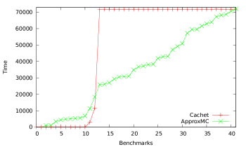
Figure 1: Performance comparison between $\mathsf{ApproxMC}$ and $\mathsf{Cachet}$. The benchmarks are arranged in increasing order of running time of $\mathsf{ApproxMC}$.

Figure 1 shows how the running times of $\mathsf{ApproxMC}$ and $\mathsf{Cachet}$ compared on this subset of our benchmarks. The y-axis in the figure represents time in seconds, while the x-axis represents benchmarks arranged in ascending order of running time of $\mathsf{ApproxMC}$. The comparison shows that although $\mathsf{Cachet}$ performed better than $\mathsf{ApproxMC}$ initially, it timed out as the “difficulty” of problems increased. $\mathsf{ApproxMC}$, however, continued to return bounds with the specified tolerance and confidence, for many more difficult and larger problems. Eventually, however, even $\mathsf{ApproxMC}$ timed out for very large problem instances. Our experiments clearly demonstrate that there is a large class of practical problems that lie beyond the reach of exact counters, but for which we can still obtain counts with $(\varepsilon,\delta)$-style guarantees in reasonable time. This suggests that given a model counting problem, it is advisable to run $\mathsf{Cachet}$ initially with a small timeout. If $\mathsf{Cachet}$ times out, $\mathsf{ApproxMC}$ should be run with a larger timeout. Finally, if $\mathsf{ApproxMC}$ also times out, counters with much weaker guarantees but shorter running times, such as bounding counters, should be used.

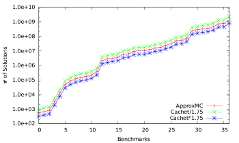
Figure 2: Quality of counts computed by $\mathsf{ApproxMC}$. The benchmarks are arranged in increasing order of model counts.

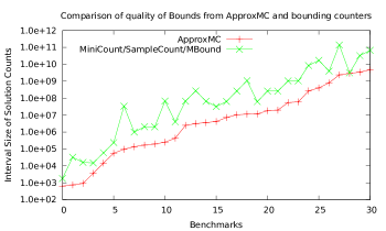
Figure 3: Comparison of interval sizes from $\mathsf{ApproxMC}$ and those from bounding counters. The benchmarks are arranged in increasing order of model counts.

Figure 2 compares the model count computed by $\mathsf{ApproxMC}$ with the bounds obtained by scaling the exact count obtained from $\mathsf{Cachet}$ by the tolerance factor ($1.75$) on a subset of our benchmarks. The y-axis in this figure represents the model count on a log-scale, while the x-axis represents the benchmarks arranged in ascending order of the model count. The figure shows that in all cases, the count reported by $\mathsf{ApproxMC}$ lies within the specified tolerance of the exact count. Although we have presented results for only a subset of our benchmarks ($37$ in total) in Figure 2 for reasons of clarity, the counts reported by $\mathsf{ApproxMC}$ were found to be within the specified tolerance of the exact counts for all $95$ benchmarks for which $\mathsf{Cachet}$ reported exact counts. We also found that the $L_{1}$ norm of the relative error, considering all $95$ benchmarks for which $\mathsf{Cachet}$ returned exact counts, was $0.033$. Thus, $\mathsf{ApproxMC}$ has approximately $4\%$ error in practice – much smaller than the theoretical guarantee of $75\%$ with $\varepsilon=0.75$.

Figure 3 compares the sizes of intervals computed using $\mathsf{ApproxMC}$ and using state-of-the-art bounding counters (as described in Section 6) on a subset of our benchmarks. The comparison clearly shows that the sizes of intervals computed using $\mathsf{ApproxMC}$ are consistently smaller than the sizes of the corresponding intervals obtained from existing bounding counters. Since smaller intervals with comparable confidence represent better approximations, we conclude that $\mathsf{ApproxMC}$ computes better approximations than a combination of existing bounding counters. In all cases, $\mathsf{ApproxMC}$ improved the upper bounds from $\mathsf{MiniCount}$ significantly; it also improved lower bounds from $\mathsf{SampleCount}$ and $\mathsf{MBound}$ to a lesser extent. For details, please refer to the full version.

8 Conclusion and Future Work

We presented $\mathsf{ApproxMC}$, the first $(\varepsilon,\delta)$ approximate counter for CNF formulae that scales in practice to tens of thousands of variables. We showed that $\mathsf{ApproxMC}$ reports bounds with small tolerance in theory, and with much smaller error in practice, with high confidence. Extending the ideas in this paper to probabilistic inference and to count models of SMT constraints is an interesting direction of future research.

References

- [1] CryptoMiniSAT. http://www.msoos.org/cryptominisat2/.
- [2] HotBits. http://www.fourmilab.ch/hotbits.
- [3] D. Angluin. On counting problems and the polynomial-time hierarchy. Theoretical Computer Science, 12(2):161 – 173, 1980.
- [4] F. Bacchus, S. Dalmao, and T. Pitassi. Algorithms and complexity results for #SAT and bayesian inference. In Proc. of FOCS, pages 340–351, 2004.
- [5] M. Bellare, O. Goldreich, and E. Petrank. Uniform generation of NP-witnesses using an NP-oracle. Information and Computation, 163(2):510–526, 1998.
- [6] E. Birnbaum and E. L. Lozinskii. The good old Davis-Putnam procedure helps counting models. Journal of Artificial Intelligence Research, 10(1):457–477, June 1999.
- [7] S. Chakraborty, K.S. Meel, and M.Y. Vardi. A scalable and nearly uniform generator of SAT witnesses. In Proc. of CAV, 2013.
- [8] A. Darwiche. New advances in compiling CNF to decomposable negation normal form. In Proc. of ECAI, pages 328–332. Citeseer, 2004.
- [9] C. Domshlak and J. Hoffmann. Probabilistic planning via heuristic forward search and weighted model counting. Journal of Artificial Intelligence Research, 30(1):565–620, 2007.
- [10] S. Ermon, C.P. Gomes, and B. Selman. Uniform solution sampling using a constraint solver as an oracle. In Proc. of UAI, 2012.
- [11] V. Gogate and R. Dechter. Samplesearch: Importance sampling in presence of determinism. Artificial Intelligence, 175(2):694–729, 2011.
- [12] C. P. Gomes, A. Sabharwal, and B. Selman. Model counting. In A. Biere, M. Heule, H. V. Maaren, and T. Walsh, editors, Handbook of Satisfiability, volume 185 of Frontiers in Artificial Intelligence and Applications, pages 633–654. IOS Press, 2009.
- [13] Carla P. Gomes, Ashish Sabharwal, and Bart Selman. Model counting: A new strategy for obtaining good bounds. In Proc. of AAAI, pages 54–61, 2006.
- [14] C.P. Gomes, J. Hoffmann, A. Sabharwal, and B. Selman. From sampling to model counting. In Proc. of IJCAI, pages 2293–2299, 2007.
- [15] C.P. Gomes, A. Sabharwal, and B. Selman. Near-uniform sampling of combinatorial spaces using XOR constraints. In Proc. of NIPS, pages 670–676, 2007.
- [16] M.R. Jerrum, L.G. Valiant, and V.V. Vazirani. Random generation of combinatorial structures from a uniform distribution. Theoretical Computer Science, 43(2-3):169–188, 1986.
- [17] R. J. Bayardo Jr. and R. Schrag. Using CSP look-back techniques to solve real-world SAT instances. In Proc. of AAAI, pages 203–208, 1997.
- [18] R.M. Karp, M. Luby, and N. Madras. Monte-Carlo approximation algorithms for enumeration problems. Journal of Algorithms, 10(3):429–448, 1989.
- [19] N. Kitchen and A. Kuehlmann. Stimulus generation for constrained random simulation. In Proc. of ICCAD, pages 258–265, 2007.
- [20] L. Kroc, A. Sabharwal, and B. Selman. Leveraging belief propagation, backtrack search, and statistics for model counting. In Proc. of CPAIOR, pages 127–141, 2008.
- [21] M. Löbbing and I. Wegener. The number of knight’s tours equals 33,439,123,484,294 – counting with binary decision diagrams. The Electronic Journal of Combinatorics, 3(1):R5, 1996.
- [22] M.G. Luby. Monte-Carlo Methods for Estimating System Reliability. PhD thesis, EECS Department, University of California, Berkeley, Jun 1983.
- [23] S. Minato. Zero-suppressed bdds for set manipulation in combinatorial problems. In Proc. of Design Automation Conference, pages 272–277, 1993.
- [24] D. Roth. On the hardness of approximate reasoning. Artificial Intelligence, 82(1):273–302, 1996.
- [25] R. Rubinstein. Stochastic enumeration method for counting np-hard problems. Methodology and Computing in Applied Probability, pages 1–43, 2012.
- [26] T. Sang, F. Bacchus, P. Beame, H. Kautz, and T. Pitassi. Combining component caching and clause learning for effective model counting. In Proc. of SAT, 2004.
- [27] T. Sang, P. Bearne, and H. Kautz. Performing bayesian inference by weighted model counting. In Prof. of AAAI, pages 475–481, 2005.
- [28] J. P. Schmidt, A. Siegel, and A. Srinivasan. Chernoff-Hoeffding bounds for applications with limited independence. SIAM Journal on Discrete Mathematics, 8:223–250, May 1995.
- [29] J. Simon. On the difference between one and many. In Proc. of ICALP, pages 480–491, 1977.
- [30] M. Sipser. A complexity theoretic approach to randomness. In Proc. of STOC, pages 330–335, 1983.
- [31] L. Stockmeyer. The complexity of approximate counting. In Proc. of STOC, pages 118–126, 1983.
- [32] M. Thurley. sharpSAT: counting models with advanced component caching and implicit bcp. In Proc. of SAT, pages 424–429, 2006.
- [33] S. Toda. On the computational power of PP and (+)P. In Proc. of FOCS, pages 514–519. IEEE, 1989.
- [34] L. Trevisan. Lecture notes on computational complexity. Notes written in Fall, 2002. http://citeseerx.ist.psu.edu/viewdoc/download?doi=10.1.1.71.9877&rep=rep1&type=pdf.
- [35] L.G. Valiant. The complexity of enumeration and reliability problems. SIAM Journal on Computing, 8(3):410–421, 1979.
- [36] W. Wei and B. Selman. A new approach to model counting. In Proc. of SAT, pages 2293–2299. Springer, 2005.
- [37] J. Yuan, A. Aziz, C. Pixley, and K. Albin. Simplifying boolean constraint solving for random simulation-vector generation. IEEE Trans. on CAD of Integrated Circuits and Systems, 23(3):412–420, 2004.