Computational Dynamic Market Risk Measures in Discrete Time Setting

Abstract

Different approaches to defining dynamic market risk measures are available in the literature. Most are focused or derived from probability theory, economic behavior or dynamic programming. Here, we propose an approach to define and implement dynamic market risk measures based on recursion and state economy representation. The proposed approach is to be implementable and to inherit properties from static market risk measures.

Key Words: Dynamic risk measures; Markov Chain; Value-at-Risk; Conditional Value-at-Risk

1 Introduction

An understanding of financial risk and related methods used to calculate risk indicators are necessary for a healthy economy, as evidenced by recent economic crises. For commercial banks, regulations and rules advocated by the Basel Committee I, II and III are in terms of minimum capital requirements, supervisory reviews and market discipline; see Basel (2005; 2010). Even if the methods used for the market risk are now well established, and the measure used is Value-at-Risk, the dynamic counterpart of this market risk is approximate. Recently, axioms have been developed for risk measures by Delbaen et al. in (Artzner et al., 1999). Proposals have been made to extend these properties to different model settings particularly to a dynamic framework in Cheridito et al. (2006, 2005); Cheridito and Kupper (2006); Jouini et al. (2008); Stadje (2010), and references therein. A recent review of the literature on dynamic market risk measures is available in Acciaio and Inner (2011). In the spirit of these studies, the problem considered here is how to build dynamic risk measures based on static measurements which can easily be implemented and which satisfy certain properties. We do so by making use of a recursion formula based on a given static risk measure ${\mathcal{R}}$ and a state economy representation modeled by a discrete Markov chain. With these approaches, the dynamic risk measure inherits properties from the static risk ${\mathcal{R}}$. The computational complexity of the dynamic risk measure is then reduced to the computational complexity of the static risk one. In term of interpretation, the Markov chain captures the uncertainties in the economy while the decision maker’s behavior is expressed via a recursion formula. The paper is organized as follows. In section 2, usual properties of market risk measures and their interpretations are briefly recalled. Then section 3 presents the recursive principle and the state economy approach to formulate dynamic market risk. These formulations of dynamic risk measures inherit properties from static risk measures. In section 4, closed formulae for recursive risk measures and Markov modulated risk measures are given through the two main market risk measures: Value-at-Risk and Conditional Value-at-Risk. An application to those two risk measures is shown when considering Gaussian and Weibull returns. The recursive Value-at-Risk presents closed formula easy to compute in the sense that at any time $t$, only the parameters of the distributions up to time $t$ are to be considered. The simulations for a ten day horizon time reveal a relatively small and stable Markov modulated risk measures which can contribute to lower the capital requirement. The conclusion is given in section 5.

2 Properties of risk measures

The usual properties of market risk measures are briefly presented, in both static and dynamic settings.

2.1 Properties of static risk measures

Consider a function ${\mathcal{R}}$ defined from a set of random variable $\mathcal{X}$ into ${\mathbb{R}}\cup\{-\infty\}\cup\{+\infty\}=\overline{{\mathbb{R}}}$. For the sake of simplicity, suppose $\mathcal{X}$ is a set of real valued random variables such that

$$\forall\,X\in\mathcal{X},\,\forall\,m\in{\mathbb{R}},\quad X+m\in\mathcal{X}.$$ (1)

Definition 1

${\mathcal{R}}$ is a (static) monetary risk measure if it satisfies the following two properties:

1. Monotonicity: $\forall\,X,\,Y\in\mathcal{X},\,\,\,X\leq Y\Rightarrow\,{\mathcal{R}}(X)\geq{\mathcal{R}}(Y)$  ,

2. Translation invariance: $\forall\,m\in{\mathbb{R}},\,\,\,{\mathcal{R}}(X+m)={\mathcal{R}}(X)-m$ .

With monotonicity, if the position $X$ is not more valuable than the position $Y$, then the risk associated with $X$ will be greater than the risk associated with $Y$. Translation invariance stipulates that additional cash decreases the risk, in particular ${\mathcal{R}}(X+{\mathcal{R}}(X))=0$.

Definition 2

A risk measure ${\mathcal{R}}$ is said to be coherent if it satisfies the properties $P_{1}$, $P_{2}$, and:

1. Sub-adititivity: $\forall\,X,Y\in\mathcal{X}$, ${\mathcal{R}}(X+Y)\leq{\mathcal{R}}(X)+{\mathcal{R}}(Y)$ ,

2. Positive homogeneity: if $k>0$ and if $X\in\mathcal{X}$ then ${\mathcal{R}}(kX)=k{\mathcal{R}}(X)$ .

With sub-additivity, the risk decreases by diversification. Positive homogeneity implies that the risk is proportional to the size of the portfolio. Further discussions on risk measure axiomatics can be found in Artzner et al. (1999; 2002).

2.2 Properties of dynamic risk measures

Fix a finite time horizon $T>0$. Contingent claims are represented by random variables $X$ defined on a probability space $(\Omega,\mathcal{F},{\mathbb{P}})$ with a filtration $(\mathcal{F}_{t})_{t\in S}$. Here $S\subset[0;T]$ is a set of times including $0$ and the time horizon $T$. In the literature, two different approaches are considered to describe dynamic market risk: either $X$ gives a final payoff at time $T$, or $X$ defines a stochastic process which takes into account payments at times $t<T$, denoted $X_{t}$. In both cases, the problem of defining dynamic risk measures that are time consistent is crucial. Time consistency expresses the way that the risk measurements at different time are interrelated. Different notions of time consistency are introduced in the literature. Here, by time consistent we mean strongly time consistent.

Consider a family of maps ${\mathcal{R}}_{t}\!\!:\;L^{\mathrm{p}}(\Omega,\mathcal{F}_{T},{\mathbb{P}})\to L^{\mathrm{p}}(\Omega,\mathcal{F}_{t},{\mathbb{P}})$. To present the properties of dynamic risk measures, assume that $X$ gives a final payoff at time $T$ and is defined on $L^{\mathrm{p}}(\Omega,\mathcal{F}_{T},{\mathbb{P}})$. Denote by ${\mathcal{R}}_{t}(X)$ the risk associated with $X$ at time $t$. ${\mathcal{R}}_{t}(X)$ is usually interpreted as a minimum capital requirement at time $t$ knowing the information $\mathcal{F}_{t}$.

The properties of a dynamic risk measure are:

• Normalization: ${\mathcal{R}}_{t}(0)=0$,

• Monotonicity: $\forall\,X,\,Y\in L^{\mathrm{p}}(\Omega,\mathcal{F}_{T},{\mathbb{P}}),\quad X\leq Y\Rightarrow{\mathcal{R}}_{t}(X)\geq{\mathcal{R}}_{t}(Y)$,

• Translation invariance: $\forall X\in L^{\mathrm{p}}(\Omega,\mathcal{F}_{T},{\mathbb{P}}),\,\forall m\in L^{\infty}(\Omega,\mathcal{F}_{t},{\mathbb{P}}),\quad{\mathcal{R}}_{t}(X+m)={\mathcal{R}}_{t}(X)-m$,

• Local property: $\forall X,Y\in L^{\mathrm{p}}(\Omega,\mathcal{F}_{T},{\mathbb{P}}),\;\forall A\in\mathcal{F}_{t},\quad{\mathcal{R}}_{t}(1_{A}X+1_{A^{c}}Y)=1_{A}{\mathcal{R}}_{t}(X)+1_{A^{c}}{\mathcal{R}}_{t}(Y)$,

• Time consistency: $\forall X,Y\in L^{\mathrm{p}}(\Omega,\mathcal{F}_{T},{\mathbb{P}}),\quad{\mathcal{R}}_{t}(X)\leq{\mathcal{R}}_{t}(Y)\Rightarrow{\mathcal{R}}_{s}(X)\leq{\mathcal{R}}_{s}(Y),\;\forall s,t\in S$ with $s\leq t$.

After normalization, a null position does not require any capital reserve to make the risk zero. The local property implies that, if the event $A$ is $\mathcal{F}_{t}$-measurable then the decision maker should know at time $t$ if $A$ has happened and adjusts his evaluation accordingly. In the literature many definitions of time consistency appear, resulting from preferences and decision policy interpretations. Time consistency is derived from the so-called Bellman principle; see (Bellman and Dreyfus, 1962; Bertsekas and Tsitsiklis, 1996).

A dynamic risk measure is convex if it satisfies $D_{1}$, $D_{2}$, $D_{3}$ and the following property:

$D_{6}$. Convexity: $\forall X,\,Y\in L^{\infty}(\Omega,\mathcal{F}_{T},{\mathbb{P}})$ and any $\eta:L^{\infty}_{+}(\Omega,\mathcal{F}_{t},{\mathbb{P}})\to[0,1]$

$${\mathcal{R}}_{t}(\eta X+(1-\eta)Y)\leq\eta{\mathcal{R}}_{t}(X)+(1-\eta){\mathcal{R}}_{t}(Y)\,,$$ (2)

where $L^{\infty}(\Omega,\mathcal{F}_{t},{\mathbb{P}})$ is the space of bounded $\mathcal{F}_{t}$-measurable random variables and $L_{+}^{\infty}(\Omega,\mathcal{F}_{t},{\mathbb{P}})\triangleq\big{\{}X\in L^{\infty}(\Omega,\mathcal{F}_{t},{\mathbb{P}})\mid{\mathbb{P}}\big{(}X\geq 0\big{)}=1\big{\}}$ . The convexity property says that diversification should decrease the risk.

The coherence property is satisfied if the maps ${\mathcal{R}}_{t}$ satisfies $D_{1}$ to $D_{5}$ and the positive homogeneity property.

$D_{7}$. Positive homogeneity:

$$\forall\,X\in L^{\mathrm{p}}(\Omega,\mathcal{F}_{T},{\mathbb{P}}),\,\forall\,m\in L_{+}^{\infty}(\Omega,\mathcal{F}_{t},{\mathbb{P}})\,\quad{\mathcal{R}}_{t}(mX)=m{\mathcal{R}}_{t}(X)\,.$$ (3)

Usually, static risk measures are associated with corresponding acceptable positions. The acceptable sets describe the set of positions which are immunized against the uncertainties. The following definition extends this notion to the dynamic case.

Definition 3

Let ${\mathcal{R}}_{t}:L^{\mathrm{p}}(\Omega,\mathcal{F}_{T},{\mathbb{P}})\to L^{\mathrm{p}}(\Omega,\mathcal{F}_{t},{\mathbb{P}})$ be a dynamic risk measure. We define the acceptable set associated with ${\mathcal{R}}_{t}$ by:

$$\mathcal{C}_{{\mathcal{R}}_{t}}:=\left\{X\in L^{\mathrm{p}}(\Omega,\mathcal{F}_{T},{\mathbb{P}})\mid{\mathcal{R}}_{t}(X)\leq 0\right\}\,.$$ (4)

The properties of a dynamic risk measure ${\mathcal{R}}_{t}$ can be expressed via the associated acceptable set $\mathcal{C}_{{\mathcal{R}}_{t}}$ and vice versa.

Proposition 1

Suppose that ${\mathcal{R}}_{t}$ satisfies the properties $D_{1}$, $D_{2}$ and $D_{3}$. Then, $\mathcal{C}_{{\mathcal{R}}_{t}}$ satisfies the following properties.

• $\mathcal{C}_{{\mathcal{R}}_{t}}$ is not empty and satisfies the following properties:

  $$\inf\{m\in L^{\mathrm{p}}(\Omega,\mathcal{F}_{T},{\mathbb{P}})\mid m\in\mathcal{C}_{{\mathcal{R}}_{t}}\}>-\infty\,,$$ (5a)

  $$\forall X\in\mathcal{C}_{{\mathcal{R}}_{t}},\,\forall\,Y\in L^{\mathrm{p}}(\Omega,\mathcal{F}_{T},{\mathbb{P}}),\quad Y\leq X\Rightarrow Y\in\mathcal{C}_{{\mathcal{R}}_{t}}\,.$$ (5b)

• Let $\mathcal{C}_{{\mathcal{R}}_{t}}$ be given. The associated dynamic risk measure ${\mathcal{R}}_{t}$ is:

  $${\mathcal{R}}_{t}(X)=ess\inf\{m\in L^{\mathrm{p}}(\Omega,\mathcal{F}_{T},{\mathbb{P}})\mid m+X\in\mathcal{C}_{{\mathcal{R}}_{t}}\}\,.$$ (6)

• ${\mathcal{R}}_{t}$ is convex if and only if the associated acceptable set $\mathcal{C}_{{\mathcal{R}}_{t}}$ is conditionally convex:

  $$\forall V,\,W\in\mathcal{C}_{{\mathcal{R}}_{t}},\quad\beta V+(1-\beta)W\in\mathcal{C}_{{\mathcal{R}}_{t}},\;\mbox{with}\;\beta\!\!:L^{\infty}_{+}(\Omega,\mathcal{F}_{t},{\mathbb{P}})\to[0,1].$$ (7)

• ${\mathcal{R}}_{t}$ is coherent if and only if the associated acceptable set $\mathcal{C}_{{\mathcal{R}}_{t}}$ is a conditionally convex cone.

Proof. See (Cheridito et al., 2006; Roorda et al., 2005). $\Box$

In the rest of this paper, we assume that $X=(X_{t})_{t\geq 0}$ is a finite dimensional stochastic process defined on the filtered probability space $(\Omega,\mathcal{F},(\mathcal{F}_{t})_{t\geq 0},{\mathbb{P}})$.

3 New formulation of dynamic risk measures

A recursive principle and a state economy approach to formulate dynamic market risk are introduced. The new formulations of dynamic risk measures are relatively easy to compute and inherit properties from static risk measures.

3.1 Dynamic risk measures based on a recursion formula

We now construct a dynamic risk measure, denoted by $({\mathcal{R}}_{t})_{t\in S}$ which is based on a static risk measure ${\mathcal{R}}\!:\mathcal{X}\to\overline{{\mathbb{R}}}$. Suppose that the time index set is discrete and finite: $S\triangleq\{0,\ldots,T\}$.

Definition 4

Suppose that a static risk measure ${\mathcal{R}}$ is given. We define a dynamic recursive risk measure by the collection of functions ${\mathcal{R}}_{t}$ given by:

$$\forall F\in\mathcal{F}_{t},\quad{\mathcal{R}}_{t}(X)\triangleq{\mathbf{1}}_{F}{\mathcal{R}}(X_{t}+{\mathcal{R}}_{t-1}(X)),\quad{\mathcal{R}}_{0}(X)\triangleq{\mathcal{R}}(X_{0}),$$ (8)

where $\forall\omega\in\Omega,\;{\mathbf{1}}_{F}(w)=1$ if $F\in\mathcal{F}_{t}$ and ${\mathbf{1}}_{F}(w)=0$ elsewhere.

The interpretation of the above definition is the following: at time $t=0$, the decision maker knows exactly the amount at risk ${\mathcal{R}}(X_{0})$. At time $t=1$, to immunize the position $X_{1}$ against uncertainties, based on his knowledge at time $t=0$, the capital ${\mathcal{R}}(X_{0})$ is required. Then, the risky position at time $t=1$ becomes $X_{1}+{\mathcal{R}}(X_{0})$. So, the capital at risk at time $t=1$ based on the risk measure ${\mathcal{R}}$ and the information generated by the stochastic process $X$ is ${\mathbf{1}}_{F}{\mathcal{R}}(X_{1}+{\mathcal{R}}(X_{0}))$. The risk at any time $t$ is then built with recursion knowing the risk at time $t-1$. The above recursion formula of dynamic risk measures is similar to the recursive utility functions developed by Epstein and Zin (1989, 1991). The principle introduced here differs from the recursion utility, where the recursion is based on information available in a planning period.

The collection of maps ${\mathcal{R}}_{t}$ inherits properties from the static risk measure ${\mathcal{R}}$.

Proposition 2

Suppose that $X$ and $Y$ are two stochastic processes.

1. Suppose that the static risk measure ${\mathcal{R}}\!\!:\mathcal{X}\to\overline{{\mathbb{R}}}$ satisfies the monotonicity property and ${\mathcal{R}}(X_{0})\leq{\mathcal{R}}(Y_{0})$. Then the dynamic recursive risk measure ${\mathcal{R}}_{t}$ is monotone.

2. Suppose that the static risk measure ${\mathcal{R}}\!\!:\mathcal{X}\to\overline{{\mathbb{R}}}$ satisfies the translation invariance property and the function ${\mathcal{R}}$ is additive. Then, the dynamic recursive risk measure ${\mathcal{R}}_{t}$ is invariant by translation.

3. Suppose that ${\mathcal{R}}\!\!:\mathcal{X}\to\overline{{\mathbb{R}}}$ is positively homogeneous and additive. Then, the associated dynamic recursive risk measure ${\mathcal{R}}_{t}$ satisfies the local property.

4. Suppose that ${\mathcal{R}}\!\!:\mathcal{X}\to\overline{{\mathbb{R}}}$ is convex and monotone. Then, the associated dynamic recursive risk measure ${\mathcal{R}}_{t}$ is convex.

We shall demonstrate $1.$; the points $2.$, $3.$ and $4.$ are straightforward.

Proof.

1. Let $X$ and $Y$ be two stochastic processes such that $X\leq Y,\;{\mathbb{P}}\,a.s$. It follows that for almost every $\omega\in\Omega$,

   $$X_{t}(\omega)\leq Y_{t}(\omega),\quad t=1,\dots,T.$$

   In particular, $X_{1}(\omega)+{\mathcal{R}}(X_{0})\leq Y_{1}(\omega)+{\mathcal{R}}(Y_{0})$. By monotonicity of ${\mathcal{R}}$ it follows that

   $$\forall F\in\mathcal{F}_{1},\quad{\mathbf{1}}_{F}{\mathcal{R}}(X_{1}+{\mathcal{R}}(X_{0}))\geq{\mathbf{1}}_{F}{\mathcal{R}}(Y_{1}+{\mathcal{R}}(Y_{0})).$$

   Then ${\mathcal{R}}_{1}(X)\geq{\mathcal{R}}_{1}(Y)$.

   By recursion,

   $$X_{t}(\omega)\leq Y_{t}(\omega)\Rightarrow{\mathcal{R}}_{t}(X)\geq{\mathcal{R}}_{t}(Y)\quad\mbox{for}\quad t=1,\ldots,T.$$

   Consequently ${\mathcal{R}}_{t}$ is monotone.

∎

Definition 5

Suppose that a dynamic recursive risk measure ${\mathcal{R}}_{t}$ is given. The corresponding acceptable sets can be defined as:

$$\mathcal{C}_{{\mathcal{R}}_{t}}\triangleq\{X\in L^{\mathrm{p}}(\Omega,\mathcal{F}_{T},{\mathbb{P}})\mid{\mathcal{R}}_{t}(X)\leq 0\}.$$ (9)

It is straightforward to see that the above acceptable set can be derived from the acceptable set of the static risk measure. Then, the acceptable sets associated with the dynamic recursive risk measure ${\mathcal{R}}_{t}$ can be expressed via the acceptable set of the static risk ${\mathcal{R}}$ and inherits its properties, as in Proposition 2.

3.2 Markov modulated dynamic risk measures

The aim of this section is to define dynamic risk measures which take into consideration the state of the economy for a given risk measure. Let $Z=\{Z_{t},t\geq 0\}$ be a discrete-time, finite state Markov chain with state space $\mathcal{Z}\triangleq\{z_{1},\ldots,z_{N}\}$ defined on the complete probability space $(\Omega,\mathcal{F},{\mathbb{P}})$. The states of $Z$ are interpreted as different states of an economy. Following (Elliott et al., 1994), we shall represent the state space of $\mathcal{Z}$ as the set of unit vectors $\mathcal{E}\triangleq\{e_{1},\ldots,e_{N}\}$ where $e_{i}=(0,\ldots,0,1,0,\ldots,0)^{\top}\in{\mathbb{R}}^{N}$ and $\top$ represents the transpose of a matrix or a vector. $Z$ then has the following semi-martingale decomposition:

$$Z_{t}=AZ_{t-1}+M_{t}\in{\mathbb{R}}^{N}\,,$$ (10)

where $A=[a_{ji}]_{i,j=1,\ldots,N}$ and $a_{ji}={\mathbb{P}}\big{(}Z_{t}=e_{j}|Z_{t-1}=e_{i}\big{)}$. $A$ is the transition matrix of the Markov chain and $M_{t}$ is a martingale increment with respect to the filtration $\mathcal{F}^{Z}$ generated by $Z$.

Assume that the stochastic processes $X$ and $Z$ are not independent. For instance, assume that, at any time $t$, there exists an $N$-vectorial real valued random variable $\widetilde{X}_{t}$ which stands for $N$ possible random variables such that

$$X_{t}=<\widetilde{X}_{t},Z_{t+1}>,\quad t=0,\ldots,T.$$ (11)

Definition 6

Suppose that the time index set is discrete and finite: $S\triangleq\{0,\ldots,T\}$. Let ${\mathcal{R}}_{t}\!\!:L^{\mathrm{p}}(\Omega,\mathcal{F}_{T},{\mathbb{P}})\to L^{\mathrm{p}}(\Omega,\mathcal{F}_{t},{\mathbb{P}})$ be a dynamic risk measure. We define the state based dynamic risk measure ${\mathcal{R}}_{t}^{Z}$ as

$${\mathcal{R}}_{t}^{Z}(X)\triangleq{\mathbb{E}}_{{\mathbb{P}}}\big{[}{\mathcal{R}}_{t}(X)|\mathcal{F}_{t}\vee\mathcal{F}_{t}^{Z}\big{]},\quad t=0,\ldots,T,$$ (12)

where $(\mathcal{F}_{t}^{Z})_{t=0,\ldots,T}$ is the filtration generated by the Markov Chain.

3.2.1 Examples of Markov modulated dynamic risk measures

Suppose that the function $F$ is a real-valued function of the Markov chain $Z$. Then, $F$ has a linear representation $F(Z_{t})={\bf F}^{\top}Z_{t}$ where ${\bf F}=({\bf F}_{1},\ldots,{\bf F}_{N})^{\top}$ and ${\bf F}_{i}=F(e_{i})$. The function $F$ can be interpreted as an aggregated value of the different states of the economy. Different Markov modulated dynamic risk measures can be considered with respect to the definition of the underlying risk measure.

Definition 7

Let a static risk measure ${\mathcal{R}}$ be given. Suppose that the dynamic risk measure is defined by:

$${\mathcal{R}}_{t}(X)={\mathcal{R}}(X_{t})<{\bf F},Z_{t+1}>,\;t=0,\ldots,T,$$ (13)

where $<\cdot,\cdot>$ states for the scalar product in ${\mathbb{R}}^{N}$. Then, the derived state based dynamic risk measure ${\mathcal{R}}^{Z}_{t}(X)\triangleq{\mathbb{E}}_{{\mathbb{P}}}\big{[}{\mathcal{R}}_{t}(X)|\mathcal{F}_{t}\vee\mathcal{F}_{t}^{Z}\big{]}$ is

$${\mathcal{R}}^{Z}_{t}(X)={\mathcal{R}}(X_{t})<{\bf F},AZ_{t}>,\;t=1,\ldots,T,$$ (14)

If ${\mathcal{R}}_{t}(X)={\mathcal{R}}(X_{t})<{\bf F},Z_{t+1}>$ then

$${\mathcal{R}}^{Z}_{t}(X) = {\mathbb{E}}\big{[}<{\mathcal{R}}(X_{t}){\bf F},Z_{t+1}>|\mathcal{F}_{t}\vee\mathcal{F}_{t}^{Z}\big{]}$$

$$= {\mathcal{R}}(X_{t})<{\bf F},AZ_{t}>.$$

If the stochastic processes $X$ and $Z$ are independent, we can still construct a Markov modulated dynamic risk measure which depends on $Z$. Let assume that any state of the economy can be associated to a particular risk measure. A possible interpretation of this statement is that the risk aversion of the decision maker depends on the state of economy. Hence, we shall consider, $N$-dimensional risk measures. Let an $N$-vectorial static risk measure $\overline{{\mathcal{R}}}$ be given, i.e. $\overline{{\mathcal{R}}}\triangleq\big{(}{\mathcal{R}}^{1},\ldots,{\mathcal{R}}^{N}\big{)}$ with ${\mathcal{R}}^{i}\!\!:\mathcal{X}\to\overline{{\mathbb{R}}}$, for $i=1,\ldots,N$. Then, different Markov modulated dynamic risk measure can be derived.

Definition 8

Assume that the dynamic risk measure is given by:

$${\mathcal{R}}_{t}(X)=<\overline{{\mathcal{R}}}(X_{t})^{\top},Z_{t+1}>,\;t=0,\ldots,T.$$ (15)

Then, the derived Markov modulated dynamic risk measure ${\mathcal{R}}^{Z}_{t}(X)\triangleq{\mathbb{E}}_{{\mathbb{P}}}\big{[}{\mathcal{R}}_{t}(X)|\mathcal{F}_{t}\vee\mathcal{F}_{t}^{Z}\big{]}$ is

$${\mathcal{R}}^{Z}_{t}(X)=<\overline{{\mathcal{R}}}(X_{t}),AZ_{t}>,\;t=1,\ldots,T,$$ (16)

where ${\mathcal{R}}^{Z}_{0}(X)\triangleq{\mathcal{R}}(X_{0})$.

Definition 9

If the dynamic risk measure $\widetilde{{\mathcal{R}}}_{t}$ is given by:

$$\widetilde{{\mathcal{R}}}_{t}(X)=<\overline{{\mathcal{R}}}_{t}(X)^{\top},Z_{t+1}>,\;t=0,\ldots,T,\;\mbox{where}\quad\overline{{\mathcal{R}}}_{t}(X)=\big{(}{\mathcal{R}}^{1}_{t},\ldots,{\mathcal{R}}^{N}_{t}\big{)},$$ (17)

and ${\mathcal{R}}^{i}_{t}(X)={\mathcal{R}}^{i}(X_{t}+{\mathcal{R}}_{t-1}^{i}(X))$, then the derived Markov modulated dynamic risk measure
$\widetilde{{\mathcal{R}}}^{Z}_{t}(X)={\mathbb{E}}_{{\mathbb{P}}}\big{[}\widetilde{{\mathcal{R}}}_{t}(X)|\mathcal{F}_{t}\vee\mathcal{F}_{t}^{Z}\big{]}$ is

$$\widetilde{{\mathcal{R}}}^{Z}_{t}(X)=<\overline{{\mathcal{R}}}_{t}(X),AZ_{t}>,\;t=1,\ldots,T,$$ (18)

where $\widetilde{{\mathcal{R}}}^{Z}_{0}(X)\triangleq{\mathcal{R}}(X_{0})$.

3.2.2 Properties of Markov modulated dynamic risk measures

The Markov modulated dynamic risk measure ${\mathcal{R}}_{t}^{Z}$ inherits properties from the associated dynamic risk measure ${\mathcal{R}}_{t}$.

Proposition 3

1. The state based dynamic risk measure ${\mathcal{R}}_{t}^{Z}$ is monotone if the associated dynamic risk measure ${\mathcal{R}}_{t}$ is monotone.

2. The state based dynamic risk measure ${\mathcal{R}}_{t}^{Z}$ satisfies the local property if and only if ${\mathcal{R}}_{t}$ satisfies the local property on $\mathcal{F}_{t}\vee\mathcal{F}_{t}^{Z}$, where $\mathcal{F}_{t}^{Z}$ stands for the filtration generated by the Markov chain $Z$.

3. The state based dynamic risk measure ${\mathcal{R}}_{t}^{Z}$ is invariant by translation if and only if ${\mathcal{R}}_{t}$ is invariant by translation on $\mathcal{F}_{t}\vee\mathcal{F}_{t}^{Z}$.

4. The state based dynamic risk measure ${\mathcal{R}}_{t}^{Z}$ is time consistent if the associated dynamic risk measure ${\mathcal{R}}_{t}$ is time consistent.

Proof.

We shall demonstrate the time consistent property. The other properties result immediately from the conditional expectation properties. Suppose that the dynamic risk measure associated with the Markov modulated dynamic risk, ${\mathcal{R}}_{t}$ is time consistent.

Suppose that $\forall\,X,Y\in L^{\mathrm{p}}(\Omega,\mathcal{F}_{T},{\mathbb{P}}),\;{\mathcal{R}}_{t}(X)\leq{\mathcal{R}}_{t}(Y)$. By monotonicity of the conditional expectation operator, it follows

$${\mathbb{E}}_{{\mathbb{P}}}\big{[}{\mathcal{R}}_{t}(X)|\mathcal{F}_{t}\vee\mathcal{F}_{t}^{Z}\big{]}\leq{\mathbb{E}}_{{\mathbb{P}}}\big{[}{\mathcal{R}}_{t}(Y)|\mathcal{F}_{t}\vee\mathcal{F}_{t}^{Z}\big{]}\Longleftrightarrow{\mathcal{R}}^{Z}_{t}(X)\leq{\mathcal{R}}^{Z}_{t}(Y),\;{\mathbb{P}}.\,a.s.$$

By time consistency of $({\mathcal{R}}_{t})_{t=1,\ldots,T}$, we have

$${\mathcal{R}}_{t}(X)\leq{\mathcal{R}}_{t}(Y)\Rightarrow{\mathcal{R}}_{t-1}(X)\leq{\mathcal{R}}_{t-1}(Y),\;{\mathbb{P}}.\,a.s.$$

It follows that ${\mathbb{E}}_{{\mathbb{P}}}\big{[}{\mathcal{R}}_{t-1}(X)|\mathcal{F}_{t-1}\vee\mathcal{F}_{t-1}^{Z}\big{]}\leq{\mathbb{E}}_{{\mathbb{P}}}\big{[}{\mathcal{R}}_{t-1}(Y)|\mathcal{F}_{t-1}\vee\mathcal{F}_{t-1}^{Z}\big{]}$. Then ${\mathcal{R}}^{Z}_{t-1}(X)\leq{\mathcal{R}}^{Z}_{t-1}(Y)$. Hence, ${\mathcal{R}}_{t}^{Z}$ is time consistent. ∎

4 Application to Value-at-Risk and Conditional Value-at-Risk

Closed formulas of recursive risk measures and Markov modulated risk measures of the Value-at-Risk and the Conditional Value-at-Risk are derived from the lemmas obtained in the previous section. An application is then given when considering Gaussian and Weibull returns. The recursive Value-at-Risk gives closed formulas easy to compute in the sense, that at any time $t$, only the parameters of the distributions up to time $t$ are to be considered. The Markov modulated risk measures appears to be relatively small and stable, which showed a benefit in term of capital management.

4.1 Value-at-Risk

Value-at-Risk, $V\!a\!R$, is the most widespread market risk measure used by the financial institutions. In $1995$, the leading 10 banks in the OECD (Basel committee) recommended this risk measure; the Basel II committee advocated $V\!a\!R$ as a standard risk measure.

Definition 10

The Value-at-Risk associated with the random variable $X$ with value in ${\mathbb{R}}$ at a level $p\in]0,1[$ is defined as the smallest $p$-quantile of $X$:

$$V\!a\!R^{p}(X)\triangleq\inf\left\{\eta\in{\mathbb{R}}:\psi_{X}(\eta)\geq p\right\},$$ (19)

where $\psi_{X}(\eta)\triangleq{\mathbb{P}}(X\leq\eta)$ defines the cumulative distribution function of $X$.

The above minimum is reached because the function $\psi_{X}$ is continuous on the left and non-decreasing. If $\psi_{X}$ is continuous and increasing, then $\eta=V\!a\!R^{p}(X)$ is the only solution of the equation $\psi_{X}(\eta)=p$. Otherwise, this latter equation could have an infinity of solutions, (when the density of $X$ is null for some value) or no solution at all, (when the density of probability is discrete).

For example, to say that the $V\!a\!R^{99\%}$ of a portfolio is equal to $\$100$ means that the maximal loss of value of the portfolio is less than a $\$100$ with a probability of $99\%$. Unfortunately, as a quantile, the $V\!a\!R$ does not take into account extreme events and it is not sub-additive. Diversification does not necessarily decrease Value-at-Risk. Consequently, $V\!a\!R$ is not coherent or convex. We extend the static Value-at-Risk defined in (19) to the dynamic framework introduced in Section 2.2. In practice, three methods are used to compute $V\!a\!R$: the historical method, the parametric method and the Monte-Carlo method. Each of them presents advantages and drawbacks. When considering the parametric method, the static $V\!a\!R$ can be extend to a dynamic framework under the hypothesis of normal distributions for the underling factors by time series estimation methods.

In fact, if at time $t$, the random variable $X_{t}\sim\mathcal{N}(\mu_{t},\sigma_{t})$ then

$$V\!a\!R^{p}(X_{t})\triangleq\mu_{t}+\sigma_{t}q_{1-p},$$ (20)

where $q_{1-p}$ stands for the quantile of the standard normal distribution. Then, the value-at-risk associated with $X_{t+1}$ can be computed once an estimation method is set to determine $\mu_{t+1}$ and $\sigma_{t+1}$ knowing $\mu_{t}$ and $\sigma_{t}$ respectively. The case where the random variable $X_{t}$ follows a Weibull distribution will also be discussed. The Weibull distribution with shape parameter less than $1$ is a common heavy tail distribution which can approximate many distribution functions. In practice, given a set of data, it is often possible to find a Weibull distribution that fits the data when the parameters of the Weibull distribution are calibrated, based on the variance and the mean of the data. Recall that, if $X_{t}$ is a generalized Weibull distribution, with parameters $\lambda_{t}>0$, $\alpha_{t}>0$ and $\theta_{t}$, i.e. $X_{t}\sim\mathcal{W}(\lambda_{t},\alpha_{t};\theta_{t})$, the associated cumulative distribution function $\psi_{X_{t}}$, is given by: (for $\eta>0$)

$$\psi_{X_{t}}(\eta)\triangleq\left\{\begin{array}[]{rl}1-e^{-\big{(}\frac{\eta-\theta_{t}}{\lambda_{t}}\big{)}^{\alpha_{t}}},&\quad\mbox{if}\quad\eta\geq\theta_{t},\\[5.69054pt] 0,&\quad\mbox{elsewhere}.\end{array}\right.$$ (21)

$V\!a\!R^{p}(X_{t})$, the value-at-risk associated with $X_{t}$ is defined by $p=\psi_{X_{t}}\big{(}V\!a\!R^{p}(X_{t}\big{)}$. Then

$$V\!a\!R^{p}(X_{t})=\displaystyle\theta_{t}+\lambda_{t}\Big{(}-\ln(1-p)\Big{)}^{\frac{1}{\alpha_{t}}}.$$ (22)

Define $X\triangleq(X_{0},X_{1},\ldots,X_{T})$.

Lemma 1

Suppose that the random return $(X_{1},\ldots,X_{T})$ are independent and identically distributed.

1. Suppose that $X_{t}\sim\mathcal{N}(\mu_{t},\sigma_{t})$ and $V\!a\!R^{p}_{0}(X)=V\!a\!R^{p}(X_{0})$. The dynamic value-at risk based on recursion associated with $X$ is:

   $$V\!a\!R^{p}_{t}(X)=\displaystyle\sum_{k=1}^{t}(-1)^{t-k}\,(\mu_{k}+\sigma_{k}q_{1-p})+(-1)^{t}\,(\mu_{0}+\sigma_{0}q_{1-p}).$$ (23)

2. Suppose that $X_{t}\sim\mathcal{W}(\lambda_{t},\alpha_{t};\theta_{t})$ such that the cumulative distribution function associated with $X_{t}$ is defined in (21), and $V\!a\!R^{p}_{0}(X)=V\!a\!R^{p}(X_{0})$. The dynamic value-at risk based on recursion associated with $X$ is:

   $$V\!a\!R^{p}_{t}(X)=\displaystyle\sum_{k=1}^{t}(-1)^{t-k}\,\Big{(}\theta_{k}+\lambda_{k}\big{(}-\ln(1-p)\big{)}^{\frac{1}{\alpha_{k}}}\Big{)}+(-1)^{t}\Big{(}\theta_{0}+\lambda_{0}\Big{(}-\ln(1-p)\Big{)}^{\frac{1}{\alpha_{0}}}\Big{)}.$$ (24)

Proof.

For $t=1$,

$$V\!a\!R^{p}_{1}(X)=V\!a\!R^{p}(X_{1}+V\!a\!R^{p}_{0}(X))=V\!a\!R^{p}\big{(}X_{1}+V\!a\!R^{p}(X_{0})\big{)}.$$

Using the invariance by translation property, it follows that

$$V\!a\!R^{p}_{1}(X)=V\!a\!R^{p}(X_{1})-V\!a\!R^{p}(X_{0}).$$

By induction, for any given time $t\geq 1$ and for any natural number $n\leq t$, $V\!a\!R^{p}_{t}(X)$ is given by:

$$V\!a\!R^{p}_{t}(X)=\displaystyle\sum_{k=t-n+1}^{t}(-1)^{t-k}\,V\!a\!R^{p}(X_{k})+(-1)^{n}\,V\!a\!R^{p}_{t-n}(X).$$ (25)

For $t=n$, we end up with the closed formula

$$V\!a\!R^{p}_{t}(X)=\displaystyle\sum_{k=1}^{t}(-1)^{t-k}\,V\!a\!R^{p}(X_{k})+(-1)^{t}\,V\!a\!R^{p}_{0}(X).$$ (26)

1. If $X_{k}\sim\mathcal{N}(\mu_{k},\sigma_{k})$, then $V\!a\!R^{p}(X_{k})=\mu_{k}+\sigma_{k}q_{1-p}$. By definition, $V\!a\!R^{p}_{0}(X)=V\!a\!R^{p}(X_{0})$. By substituting $V\!a\!R^{p}(X_{k})$ by its value in (26), we obtain the desired result.

2. If $X_{k}\sim\mathcal{W}(\lambda_{k},\alpha_{k};\theta_{k})$, then $V\!a\!R^{p}(X_{k})=\theta_{k}+\lambda_{k}\big{(}-\ln(1-p)\big{)}^{\frac{1}{\alpha_{k}}}$. Hence by substituting $V\!a\!R^{p}(X_{k})$ by its value in (26), the equality (24) is obtained.

∎

The dependence between the random returns $X_{t}$ and the state of the economy represented by the Markov chain can defined through the parameters of the density functions of the random returns, if it exists. For instance,

1. if $X_{t}\sim\mathcal{N}(\mu_{t},\sigma_{t})$, then $\mu_{t}\triangleq<\mu,Z_{t+1}>\,\mbox{and}\,\sigma_{t}\triangleq<\sigma,Z_{t+1}>$ with $\mu,\,\sigma\in{\mathbb{R}}^{N}$;

2. if $X_{t}\sim\mathcal{W}(\lambda_{t},\alpha_{t};\theta_{t})$, then $\lambda_{t}\triangleq<\lambda,Z_{t+1}>,\;\alpha_{t}\triangleq<\alpha,Z_{t+1}>$ and $\theta_{t}\triangleq<\theta,Z_{t+1}>$ with $\lambda,\,\alpha,\,\theta\in{\mathbb{R}}^{N}$.

Lemma 2

Suppose that the returns $X_{t}$ are Gaussian and independent where $\mu_{t}\triangleq<\mu,Z_{t+1}>$ and $\sigma_{t}\triangleq<\sigma,Z_{t+1}>$ with $\mu,\,\sigma\in{\mathbb{R}}^{N}$. Suppose the dynamic value-at-risk is driven by the recursion formula. Then the Markov modulated dynamic value-at-risk is

$$\Big{(}V\!a\!R^{p}_{0}\Big{)}^{Z}(X)\triangleq V\!a\!R^{p}(X_{0})\quad\mbox{and}$$ (27)

$$\Big{(}V\!a\!R^{p}_{t}\Big{)}^{Z}(X)=\displaystyle\sum_{k=1}^{t}(-1)^{t-k}\,(\overline{\mu}_{k}+\overline{\sigma}_{k}q_{1-p})+(-1)^{t}\,(\mu_{0}+\sigma_{0}q_{1-p}),$$ (28)

where

$$\overline{\mu}_{k}=<\mu A^{\top},Z_{k}>\;\mbox{and}\;\;\overline{\sigma}_{k}=<\sigma A^{\top},Z_{k}>.$$

Proof.

The $X_{t}$ are Gaussian and are independent, and ${\mathbb{E}}[Z_{t+1}\mid Z_{t}]=AZ_{t}$. ∎

Lemma 3

Suppose that $X_{t}\sim\mathcal{W}(\lambda_{t},\alpha_{t};\theta_{t})$ where $\lambda_{t}\triangleq<\lambda,Z_{t+1}>$ and $\theta_{t}\triangleq<\theta,Z_{t+1}>$ with $\lambda,\,\theta\in{\mathbb{R}}^{N}$. Suppose that the dynamic value-at-risk is driven by the recursion formula, i.e.,

$$V\!a\!R^{p}_{t}(X)=\displaystyle\sum_{k=1}^{t}(-1)^{t-k}\,\Big{(}\theta_{k}+\lambda_{k}\big{(}-\ln(1-p)\big{)}^{\frac{1}{\alpha_{k}}}\Big{)}+(-1)^{t}\Big{(}\theta_{0}+\lambda_{0}\Big{(}-\ln(1-p)\Big{)}^{\frac{1}{\alpha_{0}}}\Big{)}.$$

Then the Markov modulated dynamic value-at-risk is

$$\Big{(}V\!a\!R^{p}_{0}\Big{)}^{Z}(X)\triangleq V\!a\!R^{p}(X_{0})\quad\mbox{and}$$

$$\Big{(}V\!a\!R^{p}_{t}\Big{)}^{Z}(X)=\sum_{k=1}^{t}(-1)^{t-k}\,\Big{(}\overline{\theta}_{k}+\overline{\lambda}_{k}{\mathbb{E}}\big{[}-\big{(}\ln(1-p)\big{)}^{\frac{1}{\alpha_{k}}}\mid Z_{k}\big{]}\Big{)}+(-1)^{t}\Big{(}\theta_{0}+\lambda_{0}\Big{(}-\ln(1-p)\Big{)}^{\frac{1}{\alpha_{0}}}\Big{)},$$ (29)

where $\overline{\lambda}_{k}=<\lambda A^{\top},Z_{k}>$ and $\overline{\theta}_{k}=<\theta A^{\top},Z_{k}>$.

Proof.

The proof is immediate. ∎

4.2 Conditional Value-at-Risk

Conditional Value-at-Risk has been introduced in the financial risk literature to overcome the limitations of the $V\!a\!R$; see (Artzner et al., 1997; Embrechts et al., 1999).

Definition 11

Suppose the random variable $X\in\mathcal{X}$ has a probability density. Then the $C\!V\!a\!R$ associated is the conditional expectation defined by:

$$C\!V\!a\!R^{p}(X)\triangleq{\mathbb{E}}\big{[}X\mid X\geq VaR^{p}(X)\big{]}.$$ (30)

The following theorem allows us to rewrite the $C\!V\!a\!R$ as a solution of an optimization problem. Denote $l_{+}=\max(l,0)$. Define

$$F_{p}(X,\eta)={\mathbb{E}}\big{[}\eta+\frac{1}{1-p}(X-\eta)_{+}\big{]},$$ (31)

for any random variable $X$.

Theorem 1

For any random variable $X$ such that ${\mathbb{E}}[X]<+\infty$, the function $F_{p}(X,\cdot)$ is convex, continuously differentiable and

$$C\!V\!a\!R^{p}(X)=\min_{\eta\in{\mathbb{R}}}F_{p}(X,\eta)\,.$$ (32)

The set of solutions of the above optimization problem

$$A_{p}(X)=\displaystyle\mathop{\arg\!\min}_{\eta\in{\mathbb{R}}}F_{p}(X,\eta)$$ (33)

is non-empty, closed and bounded. Then,

$$VaR^{p}(X)\in\displaystyle\mathop{\arg\!\min}_{\eta\in{\mathbb{R}}}F_{p}(X,\eta)\,\,\mbox{ and }\,\,C\!V\!a\!R^{p}(X)=F_{p}\big{(}X,VaR^{p}(X)\big{)}.$$

Proof.

See (Rockafellar and Uryasev, 2000). ∎

With this theorem, $C\!V\!a\!R$ can be computed without any knowledge of Value-at-Risk.

Lemma 4

Suppose that the random return $(X_{1},\ldots,X_{t})$ are independent and identically distributed.

1. Suppose that the return at time $t$, $X_{t}\sim\mathcal{N}(\mu_{t},\sigma_{t})$. The dynamic conditional value-at risk based on recursion associated with $X$ is:

   $$C\!V\!a\!R^{p}_{0}(X)=C\!V\!a\!R^{p}(X_{0}),\quad\mbox{and for}\quad t=1,\ldots,T$$ (34)

   $$C\!V\!a\!R^{p}_{t}(X)=\left\{\begin{array}[]{rl}&\mu_{t}+\sigma_{t}q_{1-p}-C\!V\!a\!R^{p}_{t-1}(X),\;\mbox{if}\;X_{t}\leq V\!a\!R^{p}(L_{t})-2C\!V\!a\!R^{p}_{t-1}(X),\,{\mathbb{P}}.\;a.s\\[11.38109pt] &\mu_{t}-\frac{p}{1-p}\sigma_{t}q_{1-p}+\frac{1+p}{1-p}C\!V\!a\!R^{p}_{t-1}(X),\quad\mbox{elsewhere}.\end{array}\right.$$ (35)

2. Suppose that the return at time $t$, $X_{t}\sim\mathcal{W}(\lambda_{t},\alpha_{t};\theta_{t})$. The dynamic conditional value-at risk based on recursion associated with $X$ is:

   $$C\!V\!a\!R^{p}_{0}(X)=C\!V\!a\!R^{p}(X_{0}),\quad\mbox{and for}\quad t=1,\ldots,T$$ (36)

   $$C\!V\!a\!R^{p}_{t}(X)=\displaystyle\left\{\begin{array}[]{rl}&\theta_{t}+\lambda_{t}\big{(}-\ln(1-p)\big{)}^{\frac{1}{\alpha_{t}}}-C\!V\!a\!R^{p}_{t-1}(X),\mbox{if}\,X_{t}\leq V\!a\!R^{p}(X_{t})+2C\!V\!a\!R^{p}_{t-1}(X)\,,\\[11.38109pt] &\frac{1}{1-p}{\mathbb{E}}[X_{t}]-\frac{p}{1-p}\Big{(}\theta_{t}+\lambda_{t}\big{(}-\ln(1-p)\big{)}^{\frac{1}{\alpha_{t}}}\Big{)}+\frac{1+p}{1-p}C\!V\!a\!R^{p}_{t-1}(X),\mbox{elsewhere}.\end{array}\right.$$ (37)

Proof.

We shall prove 1. as the proof of 2. follows the same steps.

From the definition 4, the dynamic $C\!V\!a\!R^{p}_{t}$ based on recursion associated with $X$ is

$$C\!V\!a\!R^{p}_{t}(X)=C\!V\!a\!R^{p}\big{(}X_{t}+C\!V\!a\!R^{p}_{t-1}(X)\big{)}.$$

By the theorem 1, the above dynamic $C\!V\!a\!R^{p}_{t}$ can be rewritten as

$$C\!V\!a\!R^{p}_{t}(X)=V\!a\!R^{p}\big{(}X_{t}+C\!V\!a\!R^{p}_{t-1}(X)\big{)}+\frac{1}{1-p}{\mathbb{E}}\Big{[}\Big{(}X_{t}+C\!V\!a\!R^{p}_{t-1}(X)-V\!a\!R^{p}\big{(}X_{t}+C\!V\!a\!R^{p}_{t-1}(X)\big{)}\Big{)}_{+}\Big{]}.$$

From (20), $V\!a\!R^{p}\big{(}X_{t}+C\!V\!a\!R^{p}_{t-1}(X)\big{)}=\mu_{t}-C\!V\!a\!R^{p}_{t-1}(X)+\sigma_{t}q_{1-p}$. Then

$$C\!V\!a\!R^{p}_{t}(X) = \mu_{t}-C\!V\!a\!R^{p}_{t-1}(X)+\sigma_{t}q_{1-p}+\frac{1}{1-p}{\mathbb{E}}\Big{[}\Big{(}X_{t}+C\!V\!a\!R^{p}_{t-1}(X)-\mu_{t}+C\!V\!a\!R^{p}_{t-1}(X)-\sigma_{t}q_{1-p}\Big{)}_{+}\Big{]},$$

$$= \mu_{t}-C\!V\!a\!R^{p}_{t-1}(X)+\sigma_{t}q_{1-p}+\frac{1}{1-p}{\mathbb{E}}\Big{[}\Big{(}X_{t}-\mu_{t}-\sigma_{t}q_{1-p}+2C\!V\!a\!R^{p}_{t-1}(X)\Big{)}_{+}\Big{]}.$$

∎

Lemma 5

Suppose that the returns $X_{t}$ are Gaussian and independent where $\mu_{t}\triangleq<\mu,Z_{t+1}>$ and $\sigma_{t}\triangleq<\sigma,Z_{t+1}>$ with $\mu,\,\sigma\in{\mathbb{R}}^{N}$. Suppose the dynamic value-at-risk is driven by the recursion formula. Then the Markov modulated dynamic value-at-risk is

$$\Big{(}C\!V\!a\!R^{p}_{0}\Big{)}^{Z}(X)=C\!V\!a\!R^{p}(X_{0}),\quad\mbox{and for}\quad t=1,\ldots,T$$

$$\Big{(}C\!V\!a\!R^{p}_{t}\Big{)}^{Z}(X)=\left\{\begin{array}[]{rl}&\overline{\mu}_{t}+\overline{\sigma}_{t}q_{1-p},\,\mbox{if}\quad X_{t}\leq V\!a\!R^{p}(X_{t}),\\[11.38109pt] &\overline{\mu}_{t}+\frac{p}{1-p}\overline{\sigma}_{t}q_{1-p},\quad\mbox{elsewhere}.\end{array}\right.$$ (38)

Proof.

Follow the steps in the proof of Lemma 2 and use the result of Lemma 4. ∎

Lemma 6

Suppose that the returns $X_{t}\sim\mathcal{W}(\lambda_{t},\alpha_{t};\theta_{t})$ and independent where $\lambda_{t}\triangleq<\lambda,Z_{t+1}>$ and $\alpha_{t}\triangleq<\alpha,Z_{t+1}>$ with $\lambda,\,\alpha,\,\theta\in{\mathbb{R}}^{N}$. Suppose that the dynamic value-at-risk is driven by the recursion formula. Then the Markov modulated dynamic conditional value-at-risk is

$$\Big{(}C\!V\!a\!R^{p}_{0}\Big{)}^{Z}(X)=C\!V\!a\!R^{p}(X_{0}),\quad\mbox{and for}\quad t=1,\ldots,T$$

$$\Big{(}C\!V\!a\!R^{p}_{t}\Big{)}^{Z}(X)=\displaystyle\left\{\begin{array}[]{rl}&\overline{\theta}_{t}+\overline{\lambda}_{t}{\mathbb{E}}\big{[}\big{(}-\ln(1-p)\big{)}^{\frac{1}{\alpha_{t}}}\mid Z_{t}\big{]}-\big{(}C\!V\!a\!R^{p}\big{)}^{Z}_{t-1}(X),\\[5.69054pt] &\hskip 85.35826pt\mbox{if}\,X_{t}\leq\big{(}V\!a\!R^{p}\big{)}^{Z}(X_{t})+2\big{(}C\!V\!a\!R^{p}\big{)}^{Z}_{t-1}(X),\\[11.38109pt] &\frac{1}{1-p}{\mathbb{E}}[X_{t}\mid Z_{t}]-\frac{p}{1-p}\Big{(}\overline{\theta}_{t}+\overline{\lambda}_{t}{\mathbb{E}}\big{[}\big{(}-\ln(1-p)\big{)}^{\frac{1}{\alpha_{t}}}\mid Z_{t}\big{]}\Big{)}\\[5.69054pt] &\hskip 113.81102pt+\frac{1+p}{1-p}\big{(}C\!V\!a\!R^{p}_{t-1}\big{)}^{Z}(X),\mbox{elsewhere}.\end{array}\right.$$ (39)

Proof.

Follow the steps in the proof of Lemma 2 and use the result of Lemma 4. ∎

4.3 Illustration through simulation

We shall illustrate the closed dynamic risk formulas, obtained in the previous Lemmas, in two different problems. The first, illustrates dynamic risk when the random returns are Gaussian. The parameters of the Gaussian returns are calibrated based on the annual MSCI world developed market performance index between 1970 and 2009 and a Markov Chain. The second focuses on random returns which follow Weibull distributions. The parameters of the Weibull distributions are calibrated based on the historical data of a portfolio index quoted on the NYMEX market exchange, namely the global equity portfolio index. A complete risk/return report on the global equity portfolio index is also available on Bloomberg. The parameters of the Weibull distribution will depend on the state of the economy. Notice that the dynamic risk measures and the Markov modulated risk measures are relatively easy to compute. The results reveal that, the recursive risk measures and the Markov modulated risk measures are bounded above by the static risk measurements and then may lead to a lower capital requirement.

4.3.1 Gaussian returns

Assume that $X_{t}\sim\mathcal{N}(\mu_{t},\sigma_{t})$. Then $\mu_{t}\triangleq<\mu,Z_{t+1}>\,\mbox{and}\,\sigma_{t}\triangleq<\sigma,Z_{t+1}>$ with $\mu,\,\sigma\in{\mathbb{R}}^{N}$, where $N=2$. To calibrate $\mu_{t}$ and $\sigma_{t}$, assume that the return of a risky asset $X\sim\mathcal{N}(M,\Sigma)$ (with an initial investment of $1 000 US) where the mean and the standard deviation are calibrated based on the annual MSCI world developed market performance index between 1970 and 2009. Hence the mean is M=$1 113.3425 US dollars and the standard deviation is $\Sigma$=$186.29 US. Then, write $\mu\triangleq\big{[}M\!*\!1.05\;\;\;M\!*\!0.95\big{]}$ and $\sigma\triangleq\big{[}\Sigma\!*\!1.05\;\;\;\Sigma\!*\!0.95\big{]}$. For the Markov chain, assume that the transition matrix is

$$A=\left[\begin{array}[]{rl}0.25&0.75\\[11.38109pt] 0.35&0.65\end{array}\right],$$

such that $Z_{0}=[1\;;\;0]^{\top}$. The confidence level $p$ is fixed to $0.99$. Consider a horizon of $10$ days, which is the usual time horizon in market risk reports. We then compute and compare different definitions of market risk: static, dynamic recursive and one scenario of the Markov modulated risk. The results are gathered in Figure 1.

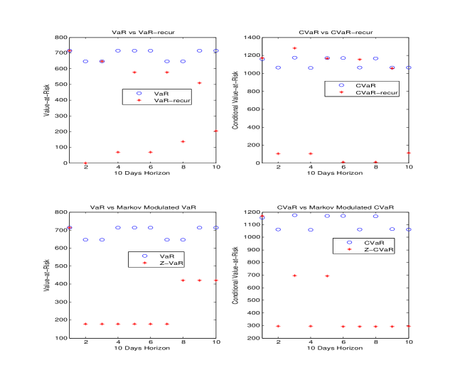
Figure 1: Dynamic Risk with Gaussian returns.

Firstly the VaR is below the CVaR, which is consistent of the fact that the VaR is lower than the CVaR. Secondly it appears that recursive and Markov modulated risk are bounded above by the static risk for both VaR and CVaR most of the time. We have plotted a trajectory of the Markov modulated risk, but more simulations confirm the same behavior. Observe that, recursive risks are more variable than the other risks in the sense that it leads to high risk on some days and low risk on other days. This is because, cash is added in the portfolio to attempt to reduce the risk.

4.3.2 Returns with Weibull Distribution

We begin by estimating the parameters of the Weibull distribution, namely $\lambda_{t}$, $\alpha_{t}$ and $\theta_{t}$. To this end, we derive $\lambda_{0}$ and $\alpha_{0}$ from real data obtained from Bloomberg and then generate $\lambda_{t}$ and $\alpha_{t}$. We suppose that $\theta_{t}=0$, for $t=0,\ldots,T$. The parameters $\lambda$ and $\alpha$ are calibrated based on the returns of the Global Equity Portfolio, quoted $BBGEX$ in Bloomberg, from $12/30/11$ to $09/27/12$. As a traded portfolio index, historical data and a complete risk report (returns, risks and risk/return ratios for different horizon times) can be obtained from Bloomberg, see Figure 2.

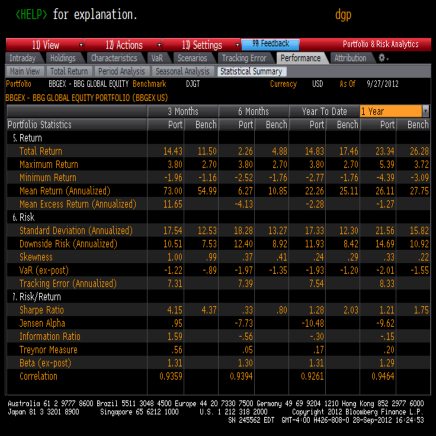
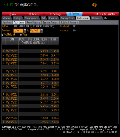
Figure 2: Historical Data and Risk Report of the Global Equity Portfolio on Bloomberg.

We then define $\lambda_{t}\triangleq<\lambda,Z_{t+1}>$ with $\lambda\in{\mathbb{R}}^{2}$, and write $\lambda\triangleq\big{[}\lambda_{0}\!*\!1.05\;\;\;\lambda_{0}\!*\!0.95\big{]}$ and $\alpha_{t}\triangleq\alpha_{0}$ for all $t=1,\ldots T$. Using the Matlab command, wblfit, the values $\lambda_{0}=6.7679$ and $\alpha_{0}=0.8016$ are obtained. The same values for the matrix of transition $A$ are used. Then different market risks are computed and compared, as shown in Figure 3.

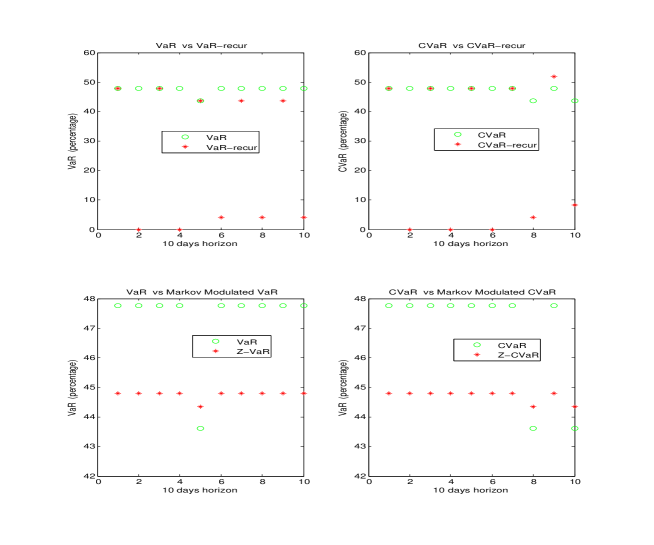
Figure 3: Dynamic Risk with Weibull returns.

The recursive and the Markov modulated risk are again well above the static risk for the VaR and the CVaR. The behavior of the recursive risk measurements are confirmed, bounded above by the static risk and null sometimes. The Markov modulated risk are relatively stable and low.

In conclusion, firstly the dynamic formulation of the market risk measure presented are relatively easy to compute and interpret, in comparison with the existing formulations in the literature. Secondly, the Markov modulated risk give lower values than the static risk and do not need as much additional cash as required for the risk based on recursion. Also, the Markov modulated risk may be preferred in terms of risk management as they lead to a lower capital requirement and give, better estimates by taking into account the state of the economy. A drawback is how to calibrate the parameters of the change rate of the economy. Are those parameters dependent on a certain category of returns, or can they be calibrated for any kind of assets? These questions are open and are crucial as the transition matrix appears in the Markov modulated risk closed formulas.

5 Conclusion

Dynamic risk measure formulas which are easy to compute, are obtained using recursive formulas and state economy representations. The dynamic risks with recursive formulas are derived from the invariant translation property. The Markov modulated risks are based on a finite state discrete Markov chain which represents the state of the economy. In both cases, the dynamic risk measures inherit properties from the initial risk measure used to express the dynamic risk measures. It appears that, at a given time $t$, the static risk measure is not necessarily greater than the recursive dynamic risk measures, and the Markov modulated risk gives lower values. It would be interesting to extend the dynamic risk formulas into a continuous time framework.

References

• Bas (2005) Chapter title. Basel lI: International Convergence of Capital Measurement and Capital Standards, Basel Committee on Banking Supervision Downloadable at: http://www.bis.org/publ/bcbs118.pdf, 2005. .
• Bas (2010) Chapter title. Basel lII: International framework for liquidity risk measurement, standards and monitoring, Basel Committee on Banking Supervision Downloadable at: http://www.bis.org/publ/bcbs188.pdf, 2010. .
• Acciaio and Inner (2011) Acciaio, B. and Inner, I., 2011. In: Dynamic risk measures., 1–34 New York: In G. Di Nunno and B. Öksendal (Eds.), Advanced Mathematical Methods for Finance, Springer.
• Artzner et al. (1997) Artzner, P., et al., 1997. Thinking coherently of risk. Risk, 10 (11), 68–71.
• Artzner et al. (1999) Artzner, P., et al., 1999. Coherent measures of risk. Mathematical Finance, 9, 203–228.
• Artzner et al. (2002) Artzner, P., et al., 2002. Coherent multiperiod risk measurement. Working Paper dowloadable at http://www.math.ethz.ch/~delbaen.
• Bellman and Dreyfus (1962) Bellman, R. and Dreyfus, S., 1962. Applied dynamic programming. Princeton: Princeton University Press.
• Bertsekas and Tsitsiklis (1996) Bertsekas, D.P. and Tsitsiklis, J.N., 1996. Neuro-Dynamic Programming. Belmont: Athena Scientific.
• Cheridito et al. (2005) Cheridito, P., Delbaen, F., and Kupper, M., 2005. Coherent and convex monetary risk measures for unbounded càdlàg processes. Finance Stochastic, 9 (3), 369–387.
• Cheridito et al. (2006) Cheridito, P., Delbaen, F., and Kupper, M., 2006. Dynamic monetary risk measures for bounded discrete-time processes. Electronic Journal of Probability, 11 (3), 57–106.
• Cheridito and Kupper (2006) Cheridito, P. and Kupper, M., 2006. Composition of time-consistent dynamic monetary risk measures in discrete time. Preprint.
• Elliott et al. (1994) Elliott, R.J., Aggoun, L., and Moore, J.B., 1994. Hidden Markov models: estimation and control. Berlin, Heidelberg, New York: Springer.
• Embrechts et al. (1999) Embrechts, P., Resnick, S., and Samorodnitsky, G., 1999. Extreme value theory as a risk management tool. North American Actuarial Journal, 3 (2), 32–41.
• Epstein and Zin (1989) Epstein, L. and Zin, S., 1989. Substitution, risk aversion and the temporal behavior of consumption and asset returns: a theoretical framework. Econometrica, 57, 937–969.
• Epstein and Zin (1991) Epstein, L. and Zin, S., 1991. Substitution, risk aversion and the temporal behavior of consumption and asset returns: an empirical analysis. Journal of Political Economy, 99, 263–286.
• Jouini et al. (2008) Jouini, E., Schachermayer, W., and Touzi, N., 2008. Optimal Risk Sharing for Law Invariant monetary utility functions. Journal of Mathematical Finance, 18, 269–292.
• Rockafellar and Uryasev (2000) Rockafellar, R.T. and Uryasev, S., 2000. Optimization of Conditional Value-at-Risk. Journal of Risk, 2, 21–41.
• Roorda et al. (2005) Roorda, B., Schumacher, J.M., and Engwerda, J., 2005. Coherent acceptability measures in multiperiod models. Mathematical Finance, 15 (4), 589–612.
• Stadje (2010) Stadje, M., 2010. Extending dynamic convex risk measures from discrete time to continuous time: A convergence approach. Journal of Insurance: Mathematics and Economics, 47, 391–404.