Dynamical Black Holes: Approach to the Final State

Abstract

Since black holes can be formed through widely varying processes, the horizon structure is highly complicated in the dynamical phase. Nonetheless, as numerical simulations show, the final state appears to be universal, well described by the Kerr geometry. How are all these large and widely varying deviations from the Kerr horizon washed out? To investigate this issue, we introduce a well-suited notion of horizon multipole moments and equations governing their dynamics, thereby providing a coordinate and slicing independent framework to investigate the approach to equilibrium. In particular, our flux formulas for multipoles can be used as analytical checks on numerical simulations and, in turn, the simulations could be used to fathom possible universalities in the way black holes approach their final equilibrium.

I Introduction

Black hole uniqueness theorems mh strongly suggest that late stages of a gravitational collapse or a black hole merger are well described by the Kerr solution. In particular, once the black hole reaches the final equilibrium, its horizon is expected to match the Kerr isolated horizon which can be characterized intrinsically, without reference to the exterior space-time lp . By now a wide variety of numerical simulations have confirmed this expectation. However, these simulations also bring out the fact that there is great diversity in the structure of the horizon during the preceding dynamical phase. At its formation, the horizon of the final black hole generically exhibits large, time-dependent distortions. Heuristically, its intrinsic geometry appears to have many ‘bumps’ and there is no simple relation between its rotational state and the spin vector of the final black hole. However, in the process of settling down to equilibrium, the Einstein dynamics manages to wash away these apparently large deviations leaving behind the Kerr isolated horizon. How does this come about? Can one provide a precise mathematical description of this approach to equilibrium? Does it carry a clear imprint of general relativity that could perhaps be seen in future gravitational wave observations? The final state is universal. Are there universalities associated also with the approach to this final state? Answers to these questions would provide us both a deeper conceptual understanding of the strong field regime of general relativity and suggest avenues to test the theory through its specific predictions for the non-linear, dynamical phase of black hole formation.

However, it is rather difficult to investigate these issues precisely because the dynamical processes of interest occur in the strong field regime of general relativity. Numerical simulations have provided insights but the horizon distortions seen in simulations often refer to components of geometrical tensors in coordinate systems and, more importantly, foliations they use. What one needs is an invariant characterization of the horizon geometry in its dynamical phase. A natural avenue is provided by the horizon multipole moments aepv ; skb ; ro which can be interpreted as the ‘source multipole moments’ of the black hole. However, as we discuss in sections II.2 and IV.3, the current definitions are not as well-suited to investigate the approach to equilibrium as one would like.

The purpose of this article is to provide multipole moments which are well-tailored for this task and provide equations for their dynamical evolution. These moments are just sets of numbers that capture the diffeomorphism invariant content of dynamical and arbitrarily distorted horizon geometries. Their evolution provides a coordinate and slicing independent description of how black holes shed the deviations from the Kerr horizon geometry and its spin structure. These equations can be used as non-trivial checks on numerical simulations in the strong field regime and, conversely, numerical solutions of these equations will bring out universalities in the approach to equilibrium, if they exist.

This article is organized as follows. In section II we collect the material on isolated and dynamical horizons that serves as our starting point. Main results are presented in sections III and IV which also include a discussion of the relation to other definitions of multipoles in the literature skb ; ro and to vortexes and tendexes that have been used to visualize the strong field geometry near black holes vt1 ; vt2 . For the convenience of computational relativists, in section IV the ideas and equations needed for numerical simulations have been presented in a self-contained fashion. If the goal is only to use these multipoles in numerical simulations, one can skip section III and go directly to IV. In section V we discuss their relation to similar issues that have been explored in the literature, including Price’s law price1 ; price2 ; rd , the close-limit approximation pp ; gnpp , and the relation between dynamics at the horizon and at infinity eloisa ; jaramillo1 ; jaramillo2 ; lr . The Appendix collects a few analytical results on the the behavior of the key fields on the dynamical horizon $H$ in the passage to equilibrium: which of them diverge, which of them admit finite limits and which of them vanish in the limit and at what rate.

Our conventions are as follows. We use Penrose’s abstract index notation. The space-time metric $g_{ab}$ has signature -,+,+,+ and curvature tensors are defined by $2\nabla_{[a}\nabla_{b]}k_{c}=R_{abc}{}^{d}k_{d}$, $R_{ac}=R_{abc}{}^{b}$ and $R=R_{ab}g^{ab}$.

II Quasi-local horizons

This section is divided into two parts. In the first we recall the notions of isolated and dynamical horizons and their basic propertiesih-prl ; abl1 ; ak . In the second, we summarize the definition of multipoles in the axi-symmetric case aepv ; skb . These quasi-local horizons have had numerous applications, including black hole thermodynamics abl2 ; ak , construction of initial data and extraction of physics from numerical simulations dkss ; skb ; akrev ; gj ; jlj , and the definition of quantum horizons and analysis of their properties abk ; aev in loop quantum gravity.

II.1 Dynamical and isolated horizons

The notion of event horizons has played a major role in the discussion of black holes. However, it is teleological and ‘too global’ in that one needs the entire space-time evolution before one can locate it. Dynamical and isolated horizons are quasi-local notions which are free from these limitations.

A dynamical horizon (DH) $H$ is a 3-dimensional space-like sub-manifold (possibly with boundary) of space-time $(\mathcal{M},g_{ab})$, foliated by a family of 2-spheres $S$ such that:
i) Each $S$ is marginally trapped; i.e. the expansion $\Theta_{(\ell)}$ of one of the (future directed) null normals $\ell^{a}$ to each $S$ vanishes, and,
ii) The expansion $\Theta_{(n)}$ of the other (future directed) null normal is negative.

Heuristically, since $H$ is obtained by ‘stacking together’ marginally trapped surfaces (MTSs), it can be thought of as the boundary of a trapped region of space-time representing a black hole. The area of the MTSs $S$ increases in time, depicting a dynamical phase during which the black hole grows as it swallows matter and gravitational waves. Furthermore, Einstein’s equations imply that there is a detailed balance law equating the rate of growth of the area-radius $R_{S}$ of any MTS $S$ with the total flux of energy (in matter and gravitational waves) falling into the black hole across $S$ ak .

Given a DH $H$, one can show that it does not admit any MTS that is not in the foliation. Thus, the foliation by MTSs —the ‘internal structure’ of $H$— is unique. DHs naturally arise in numerical simulations where one begins with a foliation of space-time and uses efficient algorithms to zero-in on the outermost MTSs. A local existence theorem ensures that, given such an MTS, it will ‘evolve’ to a DH (provided certain generic conditions are met) ams ; amms . However, DHs are not unique: a space-time region that appears to represent a black hole can carry multiple DHs. Nonetheless, partial uniqueness theorems do exist. In particular they imply that in the numerical relativity constructions, there is a unique DH that asymptotes to the event horizon in the distant future ag . This is the situation of interest in this paper.

Once the flux of energy across the horizon becomes zero, the horizon becomes isolated. More precisely:

An isolated horizon (IH) $\Delta$ is a null, 3-dimensional sub-manifold in $(\mathcal{M},g_{ab})$, topologically $S^{2}\times R$ and equipped with a specific null normal $\bar{\ell}^{a}$ such that:
i) The expansion $\Theta_{(\bar{\ell})}$ of $\bar{\ell}^{a}$ vanishes;
ii) $\mathcal{L}_{\bar{\ell}}q_{ab}=0$; and,
iii) $(\mathcal{L}_{\bar{\ell}}D_{a}-D_{a}\mathcal{L}_{\bar{\ell}})t^{a}=0$.

Here $q_{ab}$ is the intrinsic (degenerate) metric on $\Delta$, $D$ the derivative operator induced on $\Delta$ by the space-time derivative operator $\nabla$, and $t^{b}$ is any vector field that is tangential to $\Delta$.

The fields $(q_{ab},D)$ constitute the intrinsic geometry of the IH $\Delta$. By requiring that $(q_{ab},D)$ be time-independent (with respect to the evolution defined by $\bar{\ell}^{a}$), the notion of an IH extracts from that of Killing horizons just the minimal properties to ensure that the horizon itself is in equilibrium, allowing for dynamical processes to occur arbitrarily close to it pc ; akrev . The definition ensures that neither matter nor gravitational waves fall across $\Delta$ and the area of any 2-sphere cross section of $\Delta$ is the same. Event horizons of stationary black holes are simplest examples of IHs ih-prl ; abl1 ; akrev ; gj ; jlj .

Consider formation of a black hole via gravitational collapse or merger of two compact objects, one or both of which may be black holes. We are primarily interested in the late stage of such processes, when a common DH $H$ develops and approaches an IH $\Delta$ representing the future part of the event horizon of the final black hole. Because of back-scattering of gravitational waves, in the exact theory the approach would only be asymptotic. However, in numerical simulations one invariably finds that the back scattering becomes negligible within numerical errors rather soon and $H$ joins on to $\Delta$ at some finite time. Therefore, in this paper we will focus on this situation. (The case in which the equilibrium is reached only asymptotically is in fact somewhat simpler ak ; bf .)

II.2 Mutipole moments: The axi-symmetric case

Numerical simulations invariably use convenient choices of coordinates and foliations and these choices vary from one research group to another. Therefore, the task of comparing the final results requires analytical tools to probe and compare distinct horizon geometries in an invariant fashion. Multipole moments provide such a tool. In this sub-section we will summarize the situation in the case when the horizons are axi-symmetric aepv ; skb ; akrev .

Let us begin with IHs $\Delta$. An IH $\Delta$ is said to be axi-symmetric if it admits a vector field $\varphi^{a}$ satisfying: $\mathcal{L}_{\varphi}\bar{\ell}^{a}=0,\,\,\mathcal{L}_{\varphi}q_{ab}=0$, and $(\mathcal{L}_{\varphi}D_{a}-D_{a}\mathcal{L}_{\varphi})t^{b}=0$ for all vectors $t^{a}$ tangential to $\Delta$. Thus, diffeomorphisms generated by $\varphi^{a}$ on $\Delta$ preserve its geometry. These conditions imply that $\varphi^{a}$ has an unambiguous projection on the 2-sphere of integral curves of $\bar{\ell}^{a}$ which is a rotational Killing field there.

Now, it is known that the diffeomorphism invariant content of the geometry $(q_{ab},D)$ of $\Delta$ is captured in two fields:
i) The scalar curvature $\mathcal{R}$ of $\tilde{q}_{ab}$, the induced metric on any 2-sphere cross-section $S$ of $\Delta$, and,
ii) the ‘rotational’ 1-form $\omega_{a}$ on $\Delta$ defined by $D_{a}\bar{\ell}^{a}=\omega_{a}\ell^{a}$ abl1 ; akrev .
The geometrical relation of these fields is brought out by the Weyl tensor. On any IH, the component $\Psi_{2}$ of Weyl curvature is gauge invariant and furthermore we have:

$$\Psi_{2}=\textstyle{\frac{1}{4}}\,\mathcal{R}\,+\,\textstyle{\frac{i}{2}}{\epsilon}^{ab}D_{a}\omega_{b}.$$ (1)

Here ${\epsilon}^{ab}$ is the area bi-vector on any 2-sphere cross section of $\Delta$ (and the right hand side is independent of the specific choice of the cross-section $S$). Thus, on $\Delta$, the scalar curvature $\mathcal{R}$ is essentially the same as the real part of $\Psi_{2}$ while the rotational 1-form is a potential for the imaginary part of $\Psi_{2}$. In numerical simulations, one can calculate these fields on $\Delta$. However, it is still not possible to compare the results of two different simulations because the fields live on two different 3-manifolds $\Delta$ and there is no natural identification between them. Geometric multipoles are two sets of numbers $I_{l},L_{l}$, with $l=0,1,2,\ldots$ which capture the entire diffeomorphism invariant content of these fields aepv . Therefore, to compare the results of any two simulations, it suffices to compute these numbers in each simulation and compare them. In practice, it suffices to compare just the first few multipoles.

The key idea behind the definition of multipoles is the following. Given an axi-symmetric metric $q_{ab}$ on a 2-sphere $S$, one can construct a canonical round 2-sphere metric $\mathring{q}_{ab}$ on $S$ together with a preferred rotational Killing field aepv . This structure in turn provides canonical weighting functions $Y_{l,m}$, the spherical harmonics of $\mathring{q}_{ab}$. The multipoles are now defined as:

$$I_{l,m}-iL_{l,m} := \oint_{S}[\textstyle{\frac{1}{4}}\,\mathcal{R}\,+\,\textstyle{\frac{i}{2}}\epsilon^{ab}D_{a}\omega_{b}]\,Y_{l,m}\,d^{2}V$$ (2)

$$\equiv \oint_{S}\Psi_{2}\,Y_{l,m}\,d^{2}V\,.$$ (3)

where the integral is performed on any 2-sphere cross-section $S$ of $\Delta$ and $d^{2}V$ is the volume element on $S$. Of course, because the horizon geometry is axi-symmetric, only the $m=0$ multipole moments are non-vanishing. Furthermore, $I_{0,0}$ is just $1/4$th the Gauss invariant, $I_{0,0}=2\pi$, and $L_{0,0}$ vanishes. Therefore only the $l\not=0$ moments are non-trivial.

Since each step in the construction is diffeomorphism covariant —none involved introduction of a structure other than the given axi-symmetric IH— the final numbers are diffeomorphism invariant. A given axi-symmetric horizon geometry yields these numbers and, conversely, given the numbers that arise from an axi-symmetric horizon geometry, one can reconstruct that geometry up to an overall diffeomorphism. Finally, by a simple rescaling of these geometrical multipoles, one can obtain the mass and spin multipoles associated with the horizon. Since these refer only to the horizon without any reference to the exterior space-time region, they represent the source multipoles associated with the black hole itself. Indeed, as explained in aepv , the construction suggests that one can assign a ‘surface mass density’ $\rho_{\Delta}=-(1/8\pi)M_{\Delta}\,\mathcal{R}$ and a ‘surface spin current’ $j^{\Delta}_{a}=(1/8\pi G)\omega_{a}$ to the isolated horizon $\Delta$, where $M_{\Delta}$ is the total mass of $M_{\Delta}$. By contrast, the multipole moments defined at infinity represent ‘field multipoles’ which include contributions not only from the black hole but also from the exterior gravitational field (and matter, if any). In the Newtonian theory, the two sets agree. But because of its non-Abelian character, in general relativity gravity sources gravity. Therefore the two moments differ. For the mass quadrupole in Kerr space-time, for example, the difference increases with spin and is of the order of 40% near extremality $a\sim m$ aepv .

What about dynamical horizons $H$? The diffeomorphism invariant content of the intrinsic geometry of any MTS $S$ is again encoded in the scalar curvature $\mathcal{R}$ of $S$, while the role played by the rotational 1-form is now played by $\tilde{\omega}_{a}:={\tilde{q}}_{a}{}^{b}K_{bc}{\widehat{r}}^{\,c}$ where $\tilde{q}_{ab}$ is the intrinsic 2-metric on $S$ and ${\widehat{r}}^{\,c}$ is the unit (space-like) normal to $S$ within $H$ and $K_{ab}$ is the extrinsic curvature of $H$ in space-time. Using the same motivation as on IHs, one can introduce an effective ‘mass surface density’ and an ‘angular spin current density’ on any MTS $S$ of the DH $H$ and they are given by $\rho_{S}=-(1/8\pi)M_{S}\,\mathcal{R}$ and $j^{S}_{a}=(1/8\pi G)\tilde{\omega}_{a}$, where $\mathcal{R}$ is the scalar curvature of the 2-metric $\tilde{q}_{ab}$ on $S$ akrev ; skb . Therefore, in the numerical relativity literature the definition (2) has been recast in terms of these fields,

$$I_{l,m}[S]-iL_{l,m}[S]:=\oint_{S}[\textstyle{\frac{1}{4}}\,\mathcal{R}\,+\,\textstyle{\frac{i}{2}}\epsilon^{ab}\tilde{D}_{a}\tilde{\omega}_{b}]\,\,Y_{l,m}\,d^{2}V,\quad{\rm where}\quad\tilde{\omega}_{a}=\tilde{q}_{a}{}^{b}K_{bc}{\widehat{r}}^{\,c}\,,$$ (4)

and taken over to assign multipole moments $I_{l,0},\,L_{l,0}$ with each marginally trapped surface $S$ in the foliation skb . (Note that, whenever there is possible ambiguity, we use tilde over symbols that refer to 2-dimensional fields on the MTSs.)

On a DH, these multipole moments change in time, capturing the ‘intrinsic’ dynamics of the black hole, encapsulated in the horizon geometry. However, to implement this strategy, one has to find an axial symmetry $\varphi^{a}$ on each $S$. There are efficient numerical algorithms to locate this required axial Killing field $\varphi^{a}$, if it exists dkss ; kvf1 ; kvf2 ; kvf3 ; kvf4 . However, as one might expect, the DH formed in a gravitational collapse or a black hole merger generically fails to be even approximately axi-symmetric except at very late time when the geometry is already close to that of the Kerr IH. Therefore the strategy is not well-suited to study how the horizon loses its ‘hair’ in its approach to the final Kerr state. Indeed, in the dynamical phase one expects the black hole spin, for example, to change not only in magnitude but also in direction, while the axi-symmetry assumption forces the angular $l=1$ momentum moment to have only the ‘z-component’. More generally, one would expect most moments to have non-zero values for $m\not=0$ and it is of significant interest to see how dynamics of general relativity forces the black hole to shed them as it approaches equilibrium. To probe this issue, in sections III and IV we will generalize the framework by going beyond axi-symmetry in a manner that is well-suited to understanding the passage to equilibrium. We will also comment on the relation of this strategy to another approach ro that has been proposed in the literature.

Remarks:

1. In recent years, there has been considerable interest in using the Kerr multipoles to test the no-hair theorems of general relativity through gravitational wave signals. Much of this analysis is based on some key ideas introduced by Ryan fr using signals arising from a compact object orbiting around a supermassive black hole. The strategy is to express the metric of the supermassive black hole at the location of the compact object as an expansion, with the Geroch-Hansen field multipoles at infinity as coefficients rg ; rh ; bs . However, it would seem that the expansion of the space-time metric in terms of the source multipoles that characterize the horizon geometry would provide a more accurate route to mapping the Kerr geometry, unless the orbiting compact object is truly in the asymptotic region, very far from the central black hole. If it is closer, then expanding the space-time metric ‘outward’ starting from the horizon ih-prl , rather than ‘inward’ from infinity, should require far fewer terms to attain the desired accuracy. There is also a conceptual advantage that one would only need to assume vacuum equations in the region between the two bodies.

2. The simple relation (1) between the fields $\mathcal{R}$ and $\omega_{a}$ and the Weyl curvature component $\Psi_{2}$ on IHs is modified on a DH. We now have

$$\mathcal{R} = \left(4\,{\rm Re}\Psi_{2}-\tilde{q}^{ab}\tilde{q}^{cd}{{\sigma}^{(\ell)}}_{ac}{\sigma}^{(n)}_{bd}\right)$$ (5)

$$2\,{\epsilon}^{ab}\tilde{D}_{a}\tilde{\omega}_{b} = \left(4\,{\rm Im}\Psi_{2}+{\epsilon}^{ab}\tilde{q}^{cd}{\sigma}^{(\ell)}_{ac}{\sigma}^{(n)}_{bd}\right)\,,$$ (6)

where ${\sigma}^{(n)}_{ab}$ and ${\sigma}^{(\ell)}_{ab}$ are the shears associated with the null normals $\ell^{a}$ and $n^{a}$ to the MTSs $S$ and $\tilde{q}^{ab}$ is the metric on $S$. Therefore, on a DH, multipoles are no longer determined by $\Psi_{2}$ alone. (When the horizon becomes isolated, ${\sigma}^{(\ell)}_{ab}$ vanishes and the extra term drops out.)

III Multipole moments of general quasi-local horizons

In this section we present the conceptual strategy which allows us to define multipole moments on general, non-axi-symmetric horizons and track their time evolution. The material is divided into four parts. In the first, we introduce the main idea behind the generalization to non-axi-symmetric contexts; in the second, we execute this strategy, in the third, we present the generalized multipoles and, in the fourth, we present ‘balance laws’ that dictate the dynamics of multipole moments.

III.1 Main ideas

The underlying strategy is the same for both sets of geometric moments $I_{l,m}$ and $L_{l,m}$. We will first describe it in detail for the geometric spin moments $L_{l,m}$ and then summarize the situation for the $I_{l,m}$. In the first part of the discussion, we will consider the isolated and dynamical horizons simultaneously. For IHs, $S$ can be any cross section (or the 2-sphere of the null generators $\bar{\ell}^{a}$) of $\Delta$ while for DHs, $S$ can be any MTS.

Let us first integrate the expression (4) for $L_{l,m}$ by parts to obtain

$$L_{l,m}[S]=-{\textstyle{\frac{1}{2}}\sqrt{\frac{2l+1}{4\pi}}\,R^{-2}}\,\,\oint_{S}\varphi^{a}_{l,m}\,\tilde{\omega}_{a}\,d^{2}V\quad{\rm where}\quad\varphi_{l,m}^{a}=\textstyle{\sqrt{\frac{4\pi}{2l+1}}\,R^{2}\,}{\epsilon}^{ab}D_{b}Y_{l,m}\,.$$ (7)

where, as before, $R$ is the area-radius of $S$ and we have introduced certain normalization factors for later convenience. Note that the $\varphi^{a}_{l,m}$ are all divergence-free on $S$ and, furthermore, they provide a complete basis on the space of divergence-free vectors. Therefore $L_{l,m}$ can be thought of as providing a linear map from a basis of divergence-free vector fields on $S$ to reals. In this respect, there is a structural similarity between multipole moments on $\Delta$ or $H$ and ‘conserved’ charges at null infinity, which can be regarded as linear maps from the generators of the Bondi-Metzner-Sachs (BMS) group to the reals scri0 ; scri1 ; scri2 ; scri3 . With multipoles, the divergence-free vector fields play the role of infinitesimal symmetries. This conceptual parallel will be useful in our discussion.

In the axi-symmetric case, we have a symmetry vector field $\varphi^{a}$ and only $L_{l,0}$ are non-zero. In the language of vector fields these correspond to moments associated with the $\varphi_{l,0}^{a}$ satisfying ${\cal L}_{\varphi}\,\varphi^{a}_{l,0}=0$. In the literature one often sets $Y_{1,0}=\sqrt{3/4\pi}\,\zeta$. Then $Y_{l,0}$ are all essentially just the Legendre polynomials in $\zeta$;  $Y_{l,0}=\sqrt{(2l+1)/4\pi}\,\,P_{l}(\zeta)$. The function $\zeta$ is singled out by the axial Killing field: $\varphi^{a}=R^{2}\,\epsilon^{ab}\tilde{D}_{b}\zeta\,\equiv\,\varphi^{a}_{1,0}$ (whence $\varphi^{a}=\varphi^{a}_{1,0}$). On a general horizon, the major obstacle has been that we do not have access to this route; without axi-symmetry, there is no preferred $\zeta$ on $S$ and hence we do not have the required basis $Y_{l,m}$ of functions.

The first step in the generalization is just to forego the preferred basis and use (7) to associate multipole moments $L_{\phi}$ with any divergence-free vector field $\phi^{a}$ on $S$:

$$L_{\phi}[S]=-{\textstyle{\frac{1}{2}}}\,\oint_{S}\phi^{a}\,\tilde{\omega}_{a}\,d^{2}V\quad{\rm where}\quad{\cal L}_{\phi}\,\epsilon^{ab}=0.$$ (8)

But since the vector fields $\phi^{a}$ are defined separately on each $S$, we need a prescription to identify vector fields that lie on different cross-sections $S$. Otherwise, we would not be able to compare multipoles associated with two different cross-sections: On an IH the definition would be ambiguous and on a DH we would not be able to study the evolution of multipoles.

On IHs the required identification is easy to achieve: consider the diffeomorphism generated by the appropriate (possibly angle dependent) multiple of the vector field $\bar{\ell}^{a}$ that maps the first cross-section $S_{1}$ to the second $S_{2}$. This natural map –the analog of the BMS super-translation at null infinity– sends divergence-free vector fields on $S_{1}$ to divergence-free vector fields on $S_{2}$. With this identification between divergence-free vector fields, it follows that multipole moments are independent of the choice of the cross-section $S$. Equivalently, we can use the 2-sphere of generators $\bar{\ell}^{a}$ of $\Delta$ for $S$ in (8). This simpler procedure makes it manifest that the multipoles $L_{\phi}$ are properties of the IH as a whole.

On DHs, on the other hand, the geometry and hence the multipoles evolve in time and we need to follow the analog of the first procedure. Now $S$ can be any one of the MTSs. Therefore, we need to construct a dynamical vector field $X^{a}$ on $H$ that provides a natural identification between the leaves of the foliation provided by MTSs. Motions along $X^{a}$ will then be interpreted as ‘time evolution’. We need this vector field $X^{a}$ to have the following four properties:

• i) The 1-parameter family of diffeomorphisms generated by $X^{a}$ on $H$ should preserve the foliation by MTSs;

• ii) It should provide an isomorphism between the space of divergence-free vector fields on any $S$ to that of divergence-free vector fields on its image;

• iii) $X^{a}$ should be constructed covariantly, using only that structure which is already available on general dynamical horizons without any symmetry; and,

• iv) If the DH is axi-symmetric, diffeomorphisms generated by $X^{a}$ should preserve the symmetry vector field $\varphi^{a}$. As we will see this will guarantee that the multipole moments given by the more general construction –that does not refer to axi-symmetry at all– do reduce to the multipoles used in the literature in the axi-symmetric case skb .

We will show that one can select, in a diffeomorphism covariant fashion, a class of vectors fields $X^{a}$ satisfying these properties on any DH and multipoles are insensitive to the choice of $X^{a}$ within this class.

III.2 Determining the dynamical vector field $X^{a}$

Since we already have a natural foliation by MTSs, any dynamical vector field $X^{a}$ on $H$ can be decomposed into a part that is orthogonal to the foliation and a part that is tangential: $X^{a}=N{\widehat{r}}^{\,a}+N^{a}$ where, as before, ${\widehat{r}}^{\,a}$ is the unit normal to each leaf of the foliation. Because $X^{a}$ must map every MTS to some other MTS, the ‘lapse’ $N$ is severely restricted. To write out the restriction explicitly, let us introduce a coordinate $v$ on $H$ such that the leaves of the foliation are given by $v={\rm const}$. Then $N=C(q^{ab}D_{a}vD_{b}v)^{-1/2}$ where $C$ is a constant and $q^{ab}$ the inverse of the intrinsic +,+,+ metric $q_{ab}$ on $H$. Without loss of generality, we can set $C=1$ making $v$ the affine parameter of the vector field $X^{a}$. This choice of ‘lapse’ is denoted by $2b$ in the literature. Thus, we have

$$X^{a}=2b\,{\widehat{r}}^{\,a}+N^{a}\quad{\rm where}\quad 2b=|Dv|^{-\textstyle\frac{1}{2}}\,,$$ (9)

and it now remains to determine the ‘shift’ $N^{a}$. We will now show that the shift is also naturally fixed by our requirements.

We will first describe the strategy. The dynamical horizon is naturally equipped with a 2-form $\epsilon_{ab}$ that serves as the area 2-form on each MTS: $\epsilon_{ab}=\epsilon_{abc}\,{\widehat{r}}^{\,c}$ where $\epsilon_{abc}$ is the volume 3-form on $H$. Had $\mathcal{L}_{2b\hat{r}}\,\epsilon_{ab}$ been zero, $2b{\widehat{r}}^{\,a}$ would have mapped divergence-free vector fields on any $S$ to divergence-free vector fields on its image and we could just set $X^{a}=2b\,{\widehat{r}}^{\,a}$, i.e. choose the shift $N^{a}$ to be zero. But this strategy is not viable because $\mathcal{L}_{2b\hat{r}}\,\epsilon_{ab}=2b\,\tilde{K}\,\epsilon_{ab}$, where $\tilde{K}$ is the trace of the extrinsic curvature of the MTS $S$ within $H$ which is necessarily non-zero because the area of these MTSs increases in time. The idea is to remedy this ‘problem’ with an appropriate choice of the shift $N^{a}$. But no matter which shift $N^{a}$ we use, we will not be able to compensate for the entire term $2b\,\tilde{K}$: Since $\mathcal{L}_{N}\,\epsilon_{ab}=(\tilde{D}_{a}N^{a})\,\epsilon_{ab}$, even with a judicious choice of the shift $N^{a}$, we can only remove the purely inhomogeneous part

$$2b\,\tilde{K}-(1/4\pi R^{2})\,\oint_{S}2b\,\tilde{K}d^{2}V\,=\,\,2b\,\tilde{K}-2\dot{R}/R$$ (10)

of $2b\,\tilde{K}$, where the area of each MTS is given by $4\pi R^{2}$, and the ‘dot’ denotes the derivative w.r.t. $v$. Then, although $\mathcal{L}_{X}\epsilon_{ab}$ will not vanish, it will be of the form $f(v)\epsilon_{ab}$, where $f(v)=2\dot{R}/R$. Clearly, this is the best one can hope for, given the fact that the area of the MTSs changes with $v$. But since $v$ is constant on any $S$, this is sufficient to guarantee that the diffeomorphisms generated by $X^{a}$ will map divergence-free vector fields on any MTS $S$ to divergence-free vector fields on its image.

Let us now implement this strategy. First, we construct a unique function $g$ on each $S$ such that:

$$\tilde{q}^{ab}\tilde{D}_{a}\tilde{D}_{b}g=-(2b\tilde{K}-2{\dot{R}}/{R})\quad\quad{\rm and}\quad\quad\oint_{S}\,g\,d^{2}V=0$$ (11)

where, as before, the tilde quantities refer to the intrinsic 2-geometry of each MTS. The existence of the solution to the first equation is guaranteed because its right hand side integrates out to zero and the second equation makes the solution unique by removing the freedom to add a constant to $g$. We then set

$$N^{a}=\tilde{q}^{ab}\tilde{D}_{b}g,\quad\quad\hbox{\rm so that}\quad\tilde{D}_{a}N^{a}=-(2b\tilde{K}-2{\dot{R}}/{R})\,$$ (12)

so that $X^{a}=2b\,{\widehat{r}}^{\,a}+N^{a}$ satisfies $\mathcal{L}_{X}\,\epsilon_{ab}=(2\dot{R}/R)\,\epsilon_{ab}$, or, $\mathcal{L}_{X}\,R^{-2}\,\epsilon_{ab}=0$. Note that, since $\tilde{K}=-(1/2)b\,\Theta_{(\bar{n})}$, and $\bar{n}^{a}$ is smooth on all of $M$, $b\,\tilde{K}$ vanishes in the limit $v\to v_{o}$. Since $\dot{R}$ also vanishes, it follows from (11) that $g$ and hence the shift $N^{a}$ vanishes on $S_{o}$ and $X^{a}$ joins on smoothly with $\bar{\ell}^{a}$ there.

By its construction, $X^{a}$ satisfies the first three of our four requirements: It is constructed covariantly, preserves the foliation, maps divergence-free vector fields on any $S$ to divergence-free vector fields on its image. It turns out that it also satisfies the fourth requirement. To see this, let us suppose the DH is axi-symmetric with an axial symmetry vector field $\varphi^{a}$. Then, since our construction of $X^{a}$ uses only the horizon geometry, it follows that $\mathcal{L}_{\varphi}X^{a}=0$. Therefore the diffeomorphisms generated by $X^{a}$ map the axi-symmetry vector field $\varphi^{a}$ on any given MTS $S$ to the axi-symmetry vector field $\varphi^{a}$ on its image. We will see in section III.3 that this implies that, in the axi-symmetric case, the multipole defined using this general strategy coincide with those defined using axi-symmetry as in skb .

Finally, what would happen if we replace the coordinate $v$ labeling the MTSs by $v^{\prime}=f(v)$, where $f$ is a monotonic function of $v$? It is straightforward to check that $X^{a}\mapsto X^{\prime}{}^{a}=\dot{f}^{-1}X^{a}$. A vector field $\phi^{a}$ which is everywhere tangential to the MTSs and divergence-free on them satisfies $\mathcal{L}_{X}\phi^{a}=0$ if and only if it satisfies $\mathcal{L}_{X^{\prime}}\phi^{a}=0$. Therefore, the ‘permissible’ divergence-free vector fields $\phi^{a}$ selected by $X^{a}$ are the same as those selected by $X^{\prime}{}^{a}$, whence the multipoles $L_{\phi}[S]$ of Eq (8) are also the same.

III.3 Generalized multipoles

We can now readily combine the results of the last two subsections to define the generalized geometric spin multipoles. We first introduce a vector field $X^{a}=2b{\widehat{r}}^{\,a}+N^{a}$ on $H$ where $2b$ is given by (9) and $N^{a}$ by (12) and (11). Using it, we can single out the admissible weighting fields $\phi^{a}$: A vector field $\phi^{a}$ on $H$ which is tangential to every MTS, and divergence-free on it, is an admissible weighting field if $\mathcal{L}_{X}\phi^{a}=0$. Note that every admissible vector field can be obtained simply by fixing a MTS $\bar{S}$, and a divergence-free vector field $\bar{\phi}^{a}$ thereon, and Lie dragging it along $X^{a}$. Given an admissible weighting field $\phi^{a}$ and a MTS $S$, we now define the spin multipole moments $L_{\phi}[S]$ following Eq. (8):

$$L_{\phi}[{S}]=-{\textstyle{\frac{1}{2}}}\,\oint_{{S}}\phi^{a}\,\tilde{\omega}_{a}\,d^{2}V\,.$$ (13)

By varying $S$ we can study the dynamical evolution of these multipoles. Our weighting fields $\phi^{a}$ are ‘time independent’ in the sense that $\mathcal{L}_{X}\,\phi^{a}=0$. Therefore the multipole moments $L_{\phi}[S]$ derive their time dependence solely from the time dependence of the horizon geometry encoded in $\tilde{\omega}_{a}$ and the 2-sphere volume element.

Next, let us discuss the extension of the second set of multipoles, $I_{l,m}$, from axi-symmetric horizons to generic ones. For this we first note that any metric 2-sphere $S$ admits an Abelian $U(1)$ connection $\Gamma_{a}$ whose curvature 2-form is determined by the scalar curvature $\mathcal{R}$ of the metric: $\tilde{D}_{[a}\Gamma_{b]}=(\mathcal{R}/4)\epsilon_{ab}$ where $\epsilon_{ab}$ the area 2-form of $S$. Therefore, one can think of repeating the above procedure, and defining the other set of multipoles simply by replacing the 1-form $\tilde{\omega}_{a}$ by $\Gamma_{a}$ in (8).

However, there is a subtlety. While $\tilde{\omega}_{a}$ is defined globally on the 2-spheres $S$, the connection 1-form $\Gamma_{a}$ has to be defined in patches: Since $\oint_{S}\tilde{D}_{[a}\Gamma_{b]}\,\epsilon^{ab}\,d^{2}V=(1/2)\oint_{S}\mathcal{R}\,d^{2}V=4\pi$, the connection 1-form is globally defined only on the non-trivial $U(1)$ bundle over $S^{2}$ with the first Chern class. But we can just fix a fiducial connection $\mathring{\Gamma}_{a}$ which is compatible with a round 2-sphere metric $\mathring{q}_{ab}$ whose area 2-form is the same as that of the given physical metric $q_{ab}$ on $S$. Then $C_{a}:=\Gamma_{a}-\mathring{\Gamma}_{a}$ is globally defined on $S$ with the property that $\tilde{D}_{[a}C_{b]}=(1/4)(\mathcal{R}-\mathring{\mathcal{R}})\epsilon_{ab}$, where $\mathring{\mathcal{R}}=2/R^{2}$ where $R$ is the area radius of $S$. Then, for each permissible vector field $\phi^{a}$ on any MTS $S$ of the horizon, we can set

$$I_{\phi}[S]={\textstyle{\frac{1}{2}}}\,\oint_{S}\phi^{a}C_{a}\,d^{2}V\quad\quad\hbox{\rm for any $\phi^{a}$ such that}\quad\mathcal{L}_{\phi}\,\epsilon_{ab}=0.$$ (14)

Although $\mathring{\Gamma}_{a}$ is arbitrary, because each $\phi^{a}$ is divergence-free, the integral is in fact independent of the choice of $\mathring{\Gamma}_{a}$ because $\oint_{S}\mathcal{R}d^{2}V=\oint_{S}\mathring{\mathcal{R}}d^{2}V=8\pi$, the Gauss invariant of a 2-sphere.

Let us summarize. Given a generic DH $H$ we have introduced a family of vector fields $X^{a}$, unique up to a rescaling by a function that is constant on each MTS. The definition of this family is covariant and constructive: Given any DH, one can construct this family using only the structure that is already available. The diffeomorphisms generated by any of these $X^{a}$ preserve the foliation by MTSs. We then defined permissible weighting fields $\phi^{a}$ on $H$; each $\phi^{a}$ is ‘time-independent’, tangential to each MTS and divergence-free on it. This family of $\phi^{a}$ refers only to the geometric structure that is naturally available on $H$. They generalize the weighting functions $Y_{l,m}$ used on axi-symmetric horizons. Given a permissible weighting field $\phi^{a}$, we use (8) and (14) to define geometric multipoles $I_{\phi}[S],\,L_{\phi}[S]$ on any MTS $S$. By varying $S$ we track its time development.

What if the DH under consideration is axi-symmetric? Then, as we saw in section III.2, the axial symmetry field $\varphi^{a}$ is guaranteed to be ‘time independent’, i.e., Lie dragged by $X^{a}$. Now, by construction, $\mathcal{L}_{X}\,R^{2}\epsilon^{ab}=0$ and, since $\varphi^{a}=R^{2}\,\epsilon^{ab}\tilde{D}_{b}\zeta$ with $\zeta$ satisfying $\oint_{S}\zeta\,d^{2}V=0$, it follows that $\mathcal{L}_{X}\,\zeta=0$. Therefore, the vector fields $\varphi^{a}_{l,0}:=R^{2}\epsilon^{ab}\,\tilde{D}_{b}\,P_{l}(\zeta)$ are all permissible in our general setting. In this setting, they define multipoles via (14) and (13). From (8) it is clear that this general definition agrees with the definition introduced in skb . Put differently, in the axi-symmetric case, the function $\zeta$ defined separately on each cross-section using the axial symmetry field $\varphi^{a}$ is automatically ‘time independent’, i.e. satisfies $\mathcal{L}_{X}\,\zeta=0$ in the language of our general setting. Therefore, with the identification $\phi^{a}=\varphi^{a}_{l,0}$, the multipoles $L_{l,0}[S]$ defined in the axi-symmetric case (4) coincide with the multipoles $L_{\phi}[S]$ defined by the more general procedure, that does not refer to axi-symmetry at all.

III.4 Balance laws

On the DH, we have balance laws which express the difference between the area radius (and in the axi-symmetric case also spin) associated with two different MTSs $S_{1}$ and $S_{2}$ and flux of energy (and angular momentum) across the portion $\Delta H$ of the DH bounded by $S_{1}$ and $S_{2}$ ak ; akrev :

$$\frac{R_{2}-R_{1}}{2G}=\int_{\Delta H}|dR|\,T_{ab}{\widehat{\tau}}^{\,a}{\ell}^{b}\,d^{3}V+\frac{1}{16\pi G}\,\int_{\Delta H}|dR|\,(|{\sigma}^{(\ell)}|^{2}+2|\zeta|^{2})\,d^{3}V\,,$$ (15)

where as before ${\sigma}^{(\ell)}_{ab}$ is the shear of the outward pointing null normal $\ell^{a}$ to the MTSs and $R$ is the area radius of the MTSs, and where $|dR|=(q^{ab}\,D_{a}RD_{b}R)^{{1/2}}$ and the vector field $\zeta^{a}$ tangential to each $S$ is defined by:

$$\zeta^{a}:=\tilde{q}^{\,ab}\,{\widehat{r}}^{\,c}\,\nabla\!_{c}{\ell}_{b}=\tilde{\omega}^{a}+\tilde{D}^{a}\ln|dR|\,.$$ (16)

For the horizon spin, we have ak ; akrev

$$J^{\varphi}[S_{2}]-J^{\varphi}[S_{1}]=-\int_{\Delta H}\left(T_{ab}{\widehat{\tau}}^{\,a}\varphi^{b}\,+\,\frac{1}{16\pi G}(K^{ab}-Kq^{ab})\,{\cal L}\,_{\varphi}{q}_{ab}\right)\,d^{3}V.$$ (17)

These two balance laws follow directly from Einstein’s equations. On the conceptual side, they are significant because (unlike, say, Hawking’s area theorem for event horizons) they provide a detailed link between the changes of physical quantities defined on $S_{2}$ and $S_{1}$ and energy and angular momentum fluxes across the portion $\Delta H$ bounded by them. In this respect, they are completely analogous to the balance laws for the Bondi energy momentum and angular momentum at null infinity. On the practical side, because the quantities that appear in the integrand of the right and side can be calculated independently of those that appear on the left side of these equations, these balance laws can serve as internal checks on accuracy of numerical simulations. We will now show that there are balance laws associated with multipole moments that share all these features.

As in section III.3, let us begin with the spin multipoles. Note first that, apart from overall constants that are needed for dimensional reasons, the spin multipole moment $L_{\phi}[S]$ of Eq. (13) is obtained simply by replacing the axial Killing vector $\varphi^{a}$ in the definition of the horizon spin ak ; akrev ,

$$J^{\varphi}[S]:=-\frac{1}{8\pi G}\,\oint_{S}\tilde{\omega}_{a}\,\varphi^{a}d^{2}V\,,$$ (18)

with any permissible divergence-free vector field $\phi^{a}$. Therefore the balance law (17) readily generalizes to:

$$L_{\phi}[S_{2}]-L_{\phi}[S_{1}]=-\int_{\Delta H}\left(4\pi GT_{ab}{\widehat{\tau}}^{\,a}{\phi}^{b}\,+\frac{1}{4}\,(K^{ab}-Kq^{ab})\,{\cal L}\,_{\phi}q_{ab}\right)\,d^{3}V.$$ (19)

This generalization also has a direct analog at null infinity, where one can introduce balance laws not just for the 4-momentum and angular momentum but for charges associated with any of the generators of the infinite dimensional BMS Lie algebra scri0 ; scri1 ; scri2 ; scri3 . Finally, we can also obtain a differential balance law directly from the definition (8) of the spin multipole moments:

$$\frac{dL_{\phi}}{dv}=-\frac{1}{2}\oint_{S}{\cal L}\,_{X}(\tilde{\omega}_{c}\phi^{c}\,\epsilon_{ab})\,=-\frac{1}{2}\,\oint_{S}\left[{\cal L}\,_{X}(\tilde{\omega}_{a})\phi^{a}+2(\dot{R}/R)\tilde{\omega}_{a}\,\phi^{a}\right]\,d^{2}V,$$ (20)

where we have used the fact that $\phi^{a}$ is a permissible weighting field. The structure of the right hand side of this equation is quite analogous to that associated with the ‘BMS-fluxes’ at null infinity scri0 ; scri1 ; scri2 ; scri3 .

As one might expect from section III.3, the situation is the same for the other set of moments, $I_{\phi}[S]$: One only has to replace $\tilde{\omega}_{a}$ with $-C_{a}=-(\Gamma_{a}-\mathring{\Gamma}_{a})$:

$$\frac{dI_{\phi}}{dv}=\frac{1}{2}\oint_{S}\left[{\cal L}\,_{X}(C_{a})\phi^{a}+2(\dot{R}/R)C_{a}\,\phi^{a}\right]\,d^{2}V.$$ (21)

IV Approach to an axi-symmetric isolated horizon

In this section we will consider the physically interesting situation in which a generic DH settles down to an axi-symmetric IH. Then, on the IH portion we can introduce a convenient basis $\varphi_{l,m}^{a}$ of divergence-free vectors using the basis functions $Y_{l,m}$ made available by axi-symmetry. By transporting them along the canonical vector field $X^{a}$ to the DH portion we will obtain a convenient basis also on the DH portion, thereby converting the multipoles $I_{\phi},L_{\phi}$ defined in section III to a set of numbers $I_{l,m},\,L_{l,m}$ also on the DH. These can be readily evaluated in numerical simulations of black hole formation to study the approach to equilibrium.

This section is of direct interest to numerical relativity because: i) one expects the final IH in physical situations to be the Kerr IH and therefore axi-symmetric; ii) these moments are better suited to unravel universalities, if any, in the approach to equilibrium; and, iii) In most circumstances it would suffice to track just the first few multipoles. Therefore, for convenience of this readership, we have attempted to make this section self-contained.

IV.1 The setting

Let us begin with a brief summary of the notation, collecting in one place the terminology used to denote the numerous fields that feature this analysis.

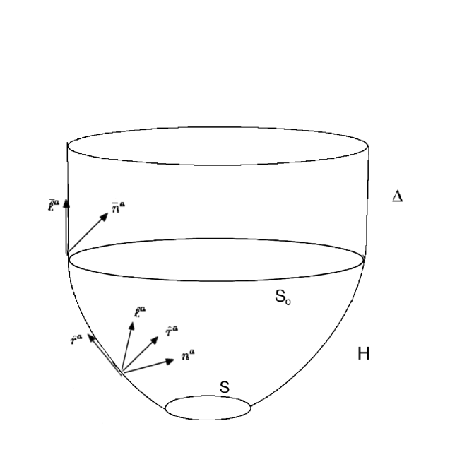
Figure 1: A quasi-local horizon $M$. The past portion of $M$ consists of a dynamical horizon $H$: this portion is space-like and foliated by marginally trapped surfaces $S$. ${\widehat{\tau}}^{a}$ is the unit time-like normal to $H$ and ${\widehat{r}}^{\,a}$ the unit space-like normal within $H$ to the foliation. Although $H$ is space-like, motions along ${\widehat{r}}^{\,a}$ can be regarded as ‘time evolution’ with respect to observers at infinity. $H$ joins on to an isolated horizon $\Delta$ in the future, representing the equilibrium state of the black hole. $\Delta$ is null, endowed with a preferred null normal $\bar{\ell}^{a}$. The transition from $H$ to $\Delta$ occurs at $S_{o}$.

Consider a quasi-local horizon $M$ with two parts: A DH $H$ in the past that is joined on to an IH at a 2-sphere cross-section $S_{o}$ (see FIG. 1). We will assume that $M$ is a 3-dimensional, $C^{k+1}$ sub-manifold of space-time and the space-time metric $g_{ab}$ is $C^{k}$ with $k\geq 2$. We will denote by $q_{ab}$ the pull-back of $g_{ab}$ to $M$; thus $q_{ab}$ has signature +,+,+ on the portion $H$ of $M$ and 0,+,+ on the portion $\Delta$. The space-time connection $\nabla_{a}$ induces a natural connection on $M$ which we denote by $D_{a}$. It satisfies $D_{a}q_{bc}=0$ on all of $M$.

The (future pointing) null normal to the IH $\Delta$ will be denoted by $\bar{\ell}^{a}$. The second (also future pointing) null normal to $S_{o}$ will be denoted by $\bar{n}^{a}$. As noted below, these null vector fields admit natural smooth extensions to $H$ and everywhere on $M$ we choose them to satisfy the normalization $\bar{\ell}^{a}\,\bar{n}_{a}=-2$. Finally, we define a 1-form $\omega_{a}$ on all of $M$ via $t^{a}\omega_{a}=-(1/2)\bar{n}_{b}t^{a}\,{\nabla_{a}}\,\bar{\ell}^{b}$ for all $t^{a}$ tangential to $M$. $\omega_{a}$ represents the rotational 1-form on $\Delta$ while, as discussed below, on $H$ it equals the $\tilde{\omega}_{a}$ defined in (4) modulo a gradient which drops out of the expression of multipole moments. We will denote the axial symmetry vector field on the IH by $\varphi^{a}$. But we do not assume that the DH is axi-symmetric. It is allowed to have arbitrary distortions in its intrinsic and extrinsic geometry.

On the dynamical horizon $H$, we will denote the unit normal to $H$ in the space-time manifold $(\mathcal{M},g_{ab})$ by ${\widehat{\tau}}^{\,a}$ and the unit normal to the MTSs $S$ within $H$ by ${\widehat{r}}^{\,a}$. Then $\ell^{a}={\widehat{\tau}}^{\,a}+{\widehat{r}}^{\,a}$ and $n^{a}={\widehat{\tau}}^{\,a}-{\widehat{r}}^{\,a}$ are the two null normals to the MTSs, with $\ell^{a}n_{a}=-2$. Let the MTSs be the level surfaces of a $C^{k+1}$ function $v$. We will assume that $S_{o}$ is the uniform limit of MTSs and is thus labeled by $v=v_{o}$. One can continue the foliation in the future on the IH such that $v$ is the affine parameter of the null normal $\bar{\ell}^{a}$. We will do so. On $H$ we set $2b=|dv|^{-1}=(q^{ab}D_{a}vD_{b}v)^{-1/2}$. The area-radius of the horizon cross-sections will be denoted by $R$; $R$ increases monotonically with $v$ and remains constant on $\Delta$. The extrinsic curvature of $H$ within space-time $(\mathcal{M},g_{ab})$ is denoted by $K_{ab}$. The intrinsic 2-metric on the MTSs $S$ is denoted by $\tilde{q}_{ab}$ and its derivative operator by $\tilde{D}_{a}$. More generally, if there is an ambiguity in the notation, we use a tilde to denote fields that are intrinsic to the MTSs.

Since $M$ is space-like in the past and null in the future, the transition at $S_{o}$ is somewhat subtle. Let us collect the basic facts (from ak ; bf and the Appendix) that are needed in the analysis of multipoles.

• i) $b^{2}$ admits a $C^{k}$ limit to $S_{o}$ and vanishes there.

• ii) On $H$ we have $\bar{\ell}^{a}=b\ell^{a}$ and $\bar{n}^{a}=b^{-1}n^{b}$. Thus, while $\ell^{a}$ is well-defined on $H$ it diverges at $S_{o}$ and cannot be extended to $\Delta$. $(\bar{\ell}^{a},\bar{n}^{a})$, on the other hand, are smooth on all of $M$.

• iii) The vector field $V^{a}:=2b\,{\widehat{r}}^{\,a}$ on $H$ admits a smooth extension to $\Delta$ and equals $\bar{\ell}^{a}$ on $\Delta$. On all of $M$, $V^{a}$ can be regarded as an evolution vector field with zero shift. Indeed, since $V^{a}D_{a}v=1$ everywhere on $M$, $v$ serves as the affine parameter of $V^{a}$. Finally, $b^{2}=V^{a}\,\bar{\ell}^{b}g_{ab}$.

• iv) If we set $\dot{R}=dR/dv$, then both $\dot{R}$ and $b$ are non-zero on $H$ but vanish on $S_{o}$ and remain zero on $\Delta$. The field $b_{o}^{2}:=b^{2}/\dot{R}$ is non-zero and smooth on $S_{o}$.

• v) the rotational 1-form $\omega_{a}$ which is well-defined everywhere on $M$ and the 1-form $\tilde{\omega}_{a}:=\tilde{q}_{a}{}^{b}\,K_{bc}\,{\widehat{r}}^{\,c}$ defined on $H$ are related by $\omega_{a}=\tilde{\omega}_{a}-\tilde{D}_{a}\ln b_{o}$.

  IV.2 Steps for numerical simulations

  The general multipole moments defined in III are somewhat abstract: Given any MTS $S$, the $I_{\phi}[S],\,L_{\phi}[S]$ can be regarded as linear mappings from permissible divergence-free vector fields $\phi^{a}$ on $H$ to real numbers. As noted in the beginning of this section, in physical situations we expect $H$ to join on to an axi-symmetric isolated horizon in the future, in fact the Kerr IH. We can exploit this extra structure by first locating a preferred basis $\varphi_{l,m}^{a}$ of divergence-free $\phi^{a}$ on $\Delta$ and then drag it along the preferred dynamical vector field $X^{a}$ (of (9), spelled out again below) to the DH portion $H$ of $M$. Put differently, we can now define the weighting functions $Y_{l,m}$ on the axi-symmetric IH and drag them down to $H$ along $X^{a}$, making them explicitly time independent. Given this basis of weighting functions, one can now replace the multipole moments $I_{\phi}[S]$ and $L_{\phi}[S]$ on $H$ with just a set of numbers $I_{l,m}[S],\,L_{l,m}[S]$ which are well-suited to study, in an invariant manner how the black hole reaches its equilibrium in any one numerical simulation. Furthermore, now one can also compare the results of two different simulations since one just has to compare numbers $I_{l,m}[S],\,L_{l,m}[S]$ associated with the MTSs $S$ with the same area. In practice the first few moments are likely to contain the most interesting information on passage to equilibrium.

  Consider, then, a numerical simulations of a black hole formation. The world tube of MTSs found after a common horizon forms provides us with the 3-manifold $M$ of FIG. 1. To extract multipole moments, one has to carry out the following steps.

  i) In the portion $H$ of $M$ on which the area of the MTSs increases monotonically, calculate the following quantities: a) The 3-metric $q_{ab}$, b) the intrinsic 2-metric $\tilde{q}_{ab}$, c) the area radius $R$ of each MTS $S$, so that the area of $S$ is $4\pi R^{2}$, d) the unit normal ${\widehat{r}}^{\,a}$ to each $S$, and, e) the trace of the extrinsic curvature $\tilde{K}$ of each $S$ within $H$.

  ii) Find the 1-form $\tilde{\omega}_{a}:=\tilde{q}_{a}{}^{b}K_{bc}\,{\widehat{r}}^{\,c}$ on each MTS S. This is the ‘seed’ that will generate the (geometric) spin moments $L_{l,m}$. Find the scalar curvature $\mathcal{R}$ of the metric $\tilde{q}_{ab}$ on each MTS $S$, which will serve as the seed for the (geometric) mass moments $I_{l,m}$. Taking the required second derivatives may introduce undesirable numerical errors (see, however, kvf3 ). If so, it may be more convenient to introduce a complex orthonormal dyad $m^{a},\bar{m}^{a}$ on each $S$ and calculate the so-called ‘spin connection’ $\Gamma_{a}$ via $\tilde{D}_{a}m_{b}=:i\Gamma_{a}m_{b}$. This 1-form $\Gamma_{a}$ can also serve as the seed to calculate the second set of moments $I_{l,m}$.

  iii) Now introduce a coordinate $v$ on $M$ such that the MTSs are the $v={\rm const}$ surfaces and the vector field $V^{a}=|dv|^{-1}{\widehat{r}}^{\,a}\equiv 2b{\widehat{r}}^{\,a}$ smoothly becomes the null normal $\bar{\ell}^{a}$ to the IH in the future region of $M$.

  iv) In the next step, construct the dynamical vector field $X^{a}$ (that will be used to transport the weighting functions $Y_{l,m}$ from the IH to the DH). On each MTS $S$, find the function $g$ via (11)

  $$\tilde{q}^{ab}\tilde{D}_{a}\tilde{D}_{b}g=-(2b\tilde{K}-2{\dot{R}}/{R})\quad\quad{\rm and}\quad\quad\oint_{S}\,g\,d^{2}V=0$$ (22)

  and define the ‘shift’ field $N^{a}$ via $N^{a}=\tilde{q}^{ab}\tilde{D}_{b}g$. Then the dynamical vector field $X^{a}$ is given by $X^{a}=V^{a}+N^{a}$. (As we approach the IH, $g$ and $N^{a}$ tend to zero and $X^{a}$ joins on smoothly with $\bar{\ell}^{a}$.)

  v) On the 2-surface $S_{o}$ where the DH $H$ joins on to the IH $\Delta$ (or anywhere to its future), find the axial Killing field $\varphi^{a}$, e.g., using the algorithm described in dkss ; kvf1 ; kvf2 ; kvf3 ; kvf4 . In practice, one would expect the geometry to become axi-symmetric within numerical errors already at late times on the DH and one can then find $\varphi^{a}$ on that MTS without having to locate $S_{o}$. On the MTS $S$ on which $\varphi^{a}$ is found, by the standard procedure developed in skb using aepv , find the basis functions $Y_{l,m}$ (defined by the canonical ‘round’ metric determined by $\varphi^{a}$ and the $\tilde{q}_{ab}$ on that MTS).

  vi) Drag these weighting functions to any MTS $S$ of interest via $\mathcal{L}_{X}Y_{lm}=0$. Construct the multipole moments $L_{l,m}$ on that $S$ using (8):

  $$L_{l,m}=-{\textstyle\frac{1}{2}}\,\oint_{S}(\epsilon^{ab}\,\tilde{D}_{b}Y_{l,m})\,\tilde{\omega}_{a}\,d^{2}V=-{\textstyle\frac{1}{2}}\,\oint_{S}(\epsilon^{ab}\,\tilde{D}_{b}Y_{l,m})\,{\omega}_{a}\,d^{2}V\,.$$ (23)

  Thus, one has to either evaluate the 1-form $\tilde{\omega}_{a}$ that refers to the extrinsic curvature $K_{ab}$ of $H$ in the 4-dimensional space-time, or the rotational 1-form $\omega_{a}$ that refers to $\bar{\ell}^{a}$ and $\bar{n}^{a}$, whichever is numerically easier. Next consider the moments $I_{l,m}$. For $l=0$, we have $I_{0,0}=2\pi$, a topological invariant. For $l\not=0$, we again have two avenues, given in the following two equivalent definitions:

  $$I_{l,m}:={\textstyle\frac{1}{4}}\,\oint_{S}\mathcal{R}\,Y_{l,m}\,d^{2}V={\textstyle\frac{1}{2}}\oint_{S}(\epsilon^{ab}\,\tilde{D}_{b}Y_{l,m})\,(\Gamma_{a}-\mathring{\Gamma}_{a})\,d^{2}V$$ (24)

  where $\mathring{\Gamma}_{a}$ is a fiducial connection; we can set $\mathring{\Gamma}_{a}=-(1/R^{2})\,\cos\theta\,\partial_{a}\phi$ in the coordinates used to express the $Y_{l,m}$. The second form may be more helpful if there are large numerical errors in computing the scalar curvature $\mathcal{R}$. Finally, the mass and spin multipoles $M_{l,m}$ and $J_{l,m}$ can be constructed by multiplying these geometric multipoles with appropriate dimensionful factors aepv ; akrev ; skb .

  This six step procedure enables one to compute the geometric multipole moments and study their evolution during the highly dynamical phase immediately after the formation of the common horizon. Computing these moments in examples is likely to bring out patterns in the way black holes shed their hair and approach the final equilibrium state, which in turn may enable one to uncover any universalities this process may have. In particular, on each MTS $S$ the procedure provides a spin vector since generically $L_{1,m}$ will be non-zero even when $m\not=0$. The ‘direction’ of the spin vector can change during the dynamical phase and the black hole would shed the $x$ and the $y$ components of this spin vector entirely as it reaches equilibrium. Does this process simply vary from case to case, depending strongly on the structure of the common horizon at its birth, or is there some underlying law that relates it to, say, the angular momentum radiated away to null infinity?

  Note that all the moments are anchored in the structure provided by the final equilibrium state of the black hole. The change in the mass dipole, for example, tells us how the black hole loses its 3-momentum with respect to its final equilibrium state. In fact a natural ‘home’ for the multipoles is provided by the tangent space at the point $i^{+}$ at future time-like infinity: The $I_{l,m}$ (or $L_{l,m}$), for example, can be naturally regarded as constituting an $l$th rank, trace-free, symmetric tensor in the tangent of $i^{+}$, all of whose indices are orthogonal to the final Bondi 4-momentum of the black hole.

  Finally, as discussed in section III.4, there are balance laws that bring out the fact that the multipoles evolve in time in response to fluxes of physical fields across the DH $H$. In section III.4 we considered the multipole moments weighted by permissible divergence-free vectors $\phi^{a}$. We now have a preferred basis $\phi^{a}_{l,m}$ constructed from spherical harmonics $Y_{l,m}$, given in Eq. (7). Therefore we can rewrite the balance laws using the $Y_{l,m}$ as weighting fields. Given two MTSs $S_{1}$ and $S_{2}$, the difference between the spin multipoles associated with them can be expressed in terms of a flux across the portion $\Delta H$ of $H$, bounded by $S_{1}$ and $S_{2}$:

  $$L_{l,m}[S_{2}]-L_{l,m}[S_{1}]=-\int_{\Delta H}\!\left(4\pi GT_{ab}{\widehat{\tau}}^{\,a}\,\epsilon^{bc}\,D_{c}Y_{l,m}\,+\frac{1}{2}(K^{ab}-Kq^{ab})\,D_{a}(\epsilon_{bc}\,D^{c}Y_{l,m})\right)\,d^{3}V\,.$$ (25)

  Similarly, for the $I_{l,m}$, we have the balance law:

  $$I_{l,m}[S_{2}]-I_{l,m}[S_{1}] = \int_{\Delta H}\frac{|dR|}{2R}\left(|{\sigma}^{(\ell)}|^{2}+2|\zeta|^{2}+16\pi GT_{ab}{\widehat{\tau}}^{\,a}{\ell}^{b}\right)Y_{l,m}d^{3}V$$ (26)

  $$+ \int_{\Delta H}|dR|\left(\frac{1}{4}Y_{l,m}\;\partial_{R}\mathcal{R}+\frac{1}{R}\zeta^{a}\partial_{a}\,Y_{l,m}\right)d^{3}V\,.$$ (27)

  On the IH, the flux integral on the right vanishes identically and the multipoles are conserved. On the DH portion, on the other hand, these balance laws could provide useful checks for numerics since the left and right sides refer to entirely different fields and they are equal only when Einstein’s equations are satisfied.

  Remarks:

  1. Throughout this analysis we have restricted ourselves to the dynamical horizon $H$ of the final black hole. Suppose we begin with two widely separated black holes which coalesce. Before the merger, we would have two distinct DHs, say $H_{1}$ and $H_{2}$. In the distant past these would join on to two distinct IHs $\Delta_{1}$ and $\Delta_{2}$, each of which would be well-modeled by a Kerr IH and hence axi-symmetric. Therefore, using the procedure described in this section, on each of these two quasi-local horizons, one would be able to define multipole moments $I_{l,m}$ and $L_{l,m}$ separately, where the required weighting functions $Y_{l,m}$ would now be transported from $\Delta_{1}$ to $H_{1}$ and from $\Delta_{2}$ to $H_{2}$. In particular, one would be able to study the evolution of the spin $L_{1,m}$ of each individual black hole. However, at present the DH framework cannot describe the merger phenomenon simply because $H_{1}\cup H_{2}\cup H$ is not a DH. Therefore, there is no simple relation between the two sets of multipoles prior to the merger and the set of multipoles after the merger.

  2. Nonetheless, using the structure available at null infinity one can discuss global balance laws. Recall first that the total Arnowitt-Deser-Misner energy-momentum is well-defined at the point $i^{o}$ at spatial infinity ah , or, equivalently, in the distant past of $\mathcal{I}^{+}$ am . Denote it by $P^{a}_{\rm initial}$. (Note that $P^{a}_{\rm initial}\not=P^{a}_{1}+P^{a}_{2}$ in general, e.g., because of the potential energy in the system.) Similarly, in the distant future, the mass monopole of the IH determines the final Bondi 4-momentum $P^{a}_{\rm final}$. Both can be thought of as living in the 4-dimensional vector space dual to the space of BMS translations. Therefore, it is meaningful to consider their difference $P^{a}_{initial}-P^{a}_{final}$ and this is precisely the Bondi 4-momentum radiated across $\mathcal{I}^{+}$ in the dynamical coalescence for which we have an independent formula am .

  The situation with angular momentum is similar but more subtle. The total (Lorentz) angular momentum of the system $M^{ab}_{\rm initial}$ is a well-defined mapping scri2 ; scri3 from the Lorentz Lie algebra of the BMS Lie algebra, picked out by the fact that the Bondi news goes to zero as one approaches $i^{o}$ np ; aa . Again, $M^{ab}_{\rm initial}$ is not simply related to $S_{1}^{a}+S_{2}^{a}$, e.g., because it also contains a contribution due to the orbital motion. The final angular momentum, $M^{ab}_{\rm final}$, on the other hand is determined entirely by the final spin of $H$ because in the distant future we only have a single black hole. However, it refers to a distinct Lorentz sub-Lie algebra of the BMS Lie algebra now selected by the fact that the Bondi news goes to zero in the distant future. (The two Lorentz sub-algebras agree only in the special circumstance in which the integral of the Bondi news along every generator of $\mathcal{I}^{+}$ vanishes np ; aa .) Therefore it is not meaningful to take the difference $M^{ab}_{\rm initial}-M^{ab}_{\rm final}$. Rather, in place of $M^{ab}_{\rm initial}$, we have to consider the angular momentum $\bar{M}^{ab}_{\rm initial}$, again evaluated in the distant past of $\mathcal{I}^{+}$ but associated with the Lorentz sub-group picked out by the Kerr geometry in the distant future. This $\bar{M}^{ab}_{\rm initial}$ is well-defined but not the same as $M^{ab}_{\rm initial}$ even conceptually. The difference $\bar{M}^{ab}_{\rm initial}-M^{ab}_{\rm final}$ is well-defined because both quantities now refer to the same Lorentz sub-group of the BMS group. Furthermore, by the balance laws scri2 ; scri3 , this is precisely the angular momentum (associated with the common Lorentz group) radiated across scri.

  To summarize, the balance laws are meaningful both for the 4-momentum and angular momentum, although in the case of angular momentum, to compare ‘apples with apples’, we have to drag the weight functions corresponding to the canonical Lorentz group in the distant future of $\mathcal{I}^{+}$ to distant past. Thus, there is no simple relation between the initial spins $S_{1}$ and $S_{2}$ of the individual black holes, the final spin $S$ of the common black hole and the angular momentum radiated away across $\mathcal{I}^{+}$. For the 4-momentum, we do have a balance law relating $P^{a}_{\rm final},\,\,P^{a}_{\rm initial}$ and the 4-momentum radiated away across $\mathcal{I}^{+}$. However, unless $P^{a}_{\rm initial}\approx P^{a}_{1}+P^{a}_{2}$, there is no simple relation between the initial 4-momenta of individual black holes and the 4-momentum of the single, final black hole.

  IV.3 Comparisons

  We will conclude section IV with a discussion of the relation of this construction with similar ideas in the literature.

  As we showed in section III, ours is a genuine generalization of the definition skb used in cases when the DH is axi-symmetric. The generalization is both technically non-trivial and conceptually important because in the early stage of the post-merger phase, the DH is generally very far from being axi-symmetric. We allowed the DH to be generic and assumed axi-symmetry only for the IH representing the final equilibrium. Nonetheless, if the entire quasi-local horizon is axi-symmetric as in skb , then on any MTS $S$ our weighting functions $Y_{l,m}$ coincide with those determined intrinsically on $S$ using the restriction of the axial symmetry $\varphi^{a}$ to $S$.

  There is another generalization in the literature, due to Owen ro . That definition has the non-trivial feature that, while it uses only the DH portion of $M$ without reference the final IH as in section III, the multipoles are a set of numbers as in section IV.2. This is achieved using a construction that is local to each MTS $S$ of the DH. In particular, the weighting functions used in ro are eigenfunctions of certain elliptic operators constructed entirely from the geometry of the MTS; one does not transport them from a final axi-symmetric state. For the mass moments, the elliptic operator is just the intrinsic Laplacian (determined by the physical metric $\tilde{q}_{ab}$) but for the spin moments a different, 4th order elliptic operator is used to ensure that, if the DH is axi-symmetric, the general procedure provides the well-established spin vector. These multipoles are distinct from ours and, generically, in the axi-symmetric case they are different also from the multipoles introduced in skb .

  The main differences from our definition are the following. First, while we use the same weighting functions for both sets of multipoles, Owen used different weighting functions. The second and more important difference is that we transport the weighting functions by dragging them from the final equilibrium configuration so that they are constant along the dynamical vector field $X^{a}$. By contrast, Owen’s weighting functions are determined by the local, time varying geometry. Owen’s construction has the advantage of being ‘local in time’, i.e., being covariant with respect to the geometry of each individual MTS. Our procedure is covariant only with respect to the geometry of the quasi-local horizon $M$ as a whole. On the other hand, because our weighting functions on any MTS are ‘the same’ as those in the final equilibrium state, our multipoles directly capture the dynamics of the horizon geometry encoded in $\mathcal{R}$ and $d\tilde{\omega}$ in the passage to equilibrium; one compares ‘apples with apples’.

  To clarify this issue of time dependence, it is useful to recall the conceptual parallel between the definition of multipoles on a DH and that of the ‘BMS charges’ at null infinity scri0 ; scri1 ; scri2 ; scri3 we used in Remark 2 at the end of section IV.2. The BMS charges are integrals over 2-sphere cross sections of null infinity of ‘seed’ physical fields, weighted by functions that refer to the BMS symmetry corresponding to the charge. (In this analogy, the cross sections of null infinity play the role of the MTS $S$ on the DH, the ‘seed’ physical fields correspond to our $\mathcal{R},d\tilde{\omega}$ on $S$, and the weighting functions, to the $Y_{l,m}$ used here.) In the BMS case, given any cross section of null infinity, using its intrinsic geometry, one can find weighting functions corresponding to a specific Lorentz sub-Lie algebra of the BMS Lie algebra and construct six charges that represent the Lorenz-angular momentum at (the retarded instant of time represented by) that cross-section. However, generically, different cross-sections select different Lorentz sub-Lie algebras of the BMS Lie algebra and therefore it is not meaningful to compare the resulting Lorentz charges on one cross section to that on another. To compare ‘apples with apples’, one has to use the same Lorentz sub-group of the BMS group. This is achieved by appropriately transporting the generators (or weighting functions) corresponding to the Lorentz subgroup used on the first cross-section to the second cross-section and carrying out the 2-sphere integral with these transported generators which, in general, are distinct from those determined intrinsically by that cross-section. Thus, the notion of the ‘same’ Lorentz sub-Lie algebra refers to the structure of the 3-dimensional null infinity as a whole; it cannot be captured by working locally on each cross-section. And it is only when the ‘same’ Lorentz generators are used that the change between the two sets of Lorentz charges refers to the change in the same physical quantities. There is no ‘contamination’ due to a change in the weighting function itself, which would have occurred if we had used the generators selected by each cross section separately.

  On quasi-local horizons, our procedure embodies this spirit in that our transport of weighting fields $Y_{l,m}$ from the final isolated horizons $\Delta$ to the dynamical horizon $H$ is analogous to the transport of the Lorentz generators which is necessary for comparisons. Therefore, our multipoles $I_{l,m}[S],\,L_{l,m}[S]$ on any MTS $S$ of the DH can be meaningfully compared to those in the final equilibrium state. They are thus well-adapted to meet the goal of this paper: capturing the physics of dynamics that makes the black hole shed its ‘hair’ in its approach to equilibrium. Owen’s goal was different. The focus there was to investigate the structure of the final state itself and the analysis provided evidence that it is Kerr. To meet that goal, it is not necessary to transport the weighting fields.

  Finally, over the last two years there has been notable interest in numerical simulations whose goal is to visualize the strong field regime around black holes in terms of the so-called ‘tendex and vortex lines’ vt1 ; vt2 . The idea is to repeat the strategy that has been so successful in electrodynamics where pictorial representations of the magnetic lines of force often provide good intuition for the complicated dynamics, e.g., in problems involving neutron stars. In the case of black holes, the gravitational lines of force are obtained using the eigen-directions of the electric and magnetic parts of the Weyl tensor,

  $$E_{ab}=C_{acbd}\tilde{\tau}^{c}\tilde{\tau}^{d}\,,\quad{\rm and}\quad B_{ab}={}^{\star}C_{acbd}\tilde{\tau}^{c}\tilde{\tau}^{d}={\textstyle{\frac{1}{2}}}\epsilon_{ac}^{\phantom{ac}pq}C_{pqbd}\tilde{\tau}^{c}\tilde{\tau}^{d},$$ (28)

  with respect to a space-time foliation to which $\tilde{\tau}^{a}$ is the unit time-like normal field. In the Kerr space-time, one can use natural foliations, the lines cross the MTSs, and their visual properties provide intuition for physical effects of the near horizon, strong gravitational field. These images are also useful when one considers perturbations around Kerr. However, in a truly non-linear, dynamical situation, e.g., at the formation of the common horizon during generic black hole collisions, there are no natural space-time foliations. Since the lines of force are tied to foliation choices that are made by extrapolating one’s intuition based on the stationary Kerr geometry (and perturbative dynamics thereon) these visual images cannot be used to draw reliable conclusions about the physics of dynamical processes in the strong field, near-horizon geometry. Multipole moments introduced in this paper serve a complementary role. In particular, it would be instructive to develop programs to visualize the distortions in the geometry and the angular momentum content of the dynamical horizon membrane. In Kerr space-times, the geometrical intuition provided by these visualizations would not be as rich as that provided by vortexes and tendexes where the lines of force extend beyond the horizon, all the way to infinity. But in the strong field and highly dynamical regime, the intuition these multipoles provide would capture a more accurate depiction of the actual, invariant physics.

  V Discussion

  There is growing evidence that, in general relativity, the final equilibrium state of black hole horizons is extremely well-approximated by the Kerr horizon. However, immediately after its formation, the common horizon that surrounds all matter and individual black holes is highly dynamical and its evolution varies from case to case. In this paper we have introduced multipole moments to gain physical insights into the strong field dynamical processes that efficiently smoothen all the distortions, leading to an universal final geometry.

  We presented two sets of ideas. The first, discussed in section III, is most useful on DHs $H$. It associates with each MTS $S$ of $H$ multipole moments $I_{\phi}[S],\,L_{\phi}[S]$, where the weighting functions $\phi$ are a set of ‘time independent’ vector fields $\phi^{a}$ which are tangential to each $S$ and divergence-free on them. On any given DH, the evolution of these multipoles captures the dynamics of the transition to equilibrium in a coordinate and slicing independent fashion. The second idea, presented in section IV, is applicable only in a setting in which the DH is joined on to an axi-symmetric IH in the future. However, from physical considerations, this is not a genuine restriction because, as we just noted, one expects the final equilibrium state to be the Kerr IH. In this case, one can introduce a convenient basis $\varphi^{a}_{l,m}$ in the space of weighting fields $\phi^{a}$, labeled by spherical harmonics $Y_{l,m}$ that are determined on $H$ in an invariant fashion by the future axi-symmetric structure. Consequently, now the multipole moments on any MTS $S$ are just a set of numbers $I_{l,m}[S],L_{l,m}[S]$. As we saw in section IV.2, their definitions are well-suited for numerical simulations. Not only can one use them to monitor dynamics on any one DH, but they also enable one to compare results of distinct simulations. (This is not possible with $I_{\phi}[S],\,L_{\phi}[S]$ because one does not have a canonical identification between the divergence-free vector fields $\phi^{a}$ on the two DHS obtained in two distinct simulations.) Also, these multipoles provide tools to physically interpret the dynamical process. For example, $L_{1,m}[S]$ provides a well-defined notion of the spin-vector during the dynamical phase. Tracking the evolution of the direction of the spin is likely to provide new insights. More generally, by explicitly evaluating a few low $l$ multipoles and monitoring their evolution, numerical simulations should be able to find any patterns or universalities in the manner black holes shed their hair. We also provided formulas for fluxes of these multipoles. Since they are strict consequences of field equations, they can serve as analytic checks on numerics in the strong field and highly dynamical regimes.

  This framework is well-suited to analyze a number of issues. Recall first that, over the years, perturbative investigations have provided strong indications that the passage to equilibrium may have some universal features. In particular, the Price’s law and increasing evidence in its favor price1 ; price2 ; rd , the success of the close limit approximation of Price and Pullin pp ; gnpp , and the universality of quasi-normal ringing price2 all suggest that, although the strong field dynamics after the formation of a common horizon is highly non-linear, it has a deep underlying simplicity. However, to date the investigations in the strong field limit have been restricted to spherical symmetry rd . In this case, there is no gravitational radiation, the DH has no hair, and its dynamics is rather simple and fully understood bi . The central questions concerning the dynamical processes that wash away the distortions and non-trivial angular momentum structure of the DH simply do not arise. Therefore, numerical studies of the time evolution of multipoles $I_{l,m}[S],\,L_{l,m}[S]$ in the general case, far removed from spherical symmetry, could lead to fresh and interesting insights. As the DH reaches its equilibrium, is there a correlation between rate at which it sheds its multipoles and, say, Price’s law? For example, recent numerical simulations suggest that the end point of the collision of two spinning black holes can be a Schwarzschild black hole jh . In this case the DH would have to lose all its multipoles except the mass monopole. Is there a pattern to how they are lost? Is it the case, as one would intuitively expect, that the high $l$-multipoles die quickly while the low $l$ are dissipated more slowly? Is there in fact a quantitative, universal behavior? Another example is provided by the ‘anti-kick’ that is associated with the post-merger phase of dynamics of binary black holes jaramillo1 . There are general arguments to suggest that it should be possible to account for this phenomenon in terms of the behavior of the mass monopole and dipole of the DH that forms after coalescence. Again, calculation of these moments and investigating their dynamics are likely to provide new physical insights.

  The physical process involved in the manner equilibrium is reached is not directly intuitive because the DH lies inside the event horizon. Consequently, it does not radiate away its multipoles to infinity. Rather, distortions in the geometry and the angular momentum structure of the DH are washed out by the radiation that falls into the black hole. But it appears that there is a correlation between what falls into the DH and what gets radiated away to null infinity. The qualitative picture is that there is some radiation in the potential just outside the event horizon, some of which falls into the black hole and the rest escapes to infinity ‘remembering’ the way it was correlated. At first this scenario can seem rather far-fetched because it is difficult to imagine processes responsible for this memory retention. But the paradigm is supported by several recent simulations eloisa ; jaramillo1 ; jaramillo2 ; lr . Multipole moments defined here should help further develop these ideas.

  Acknowledgements: We would like to thank Chris Beetle, Jonathan Engle, James Healy, Jose Jaramillo, Pablo Laguna, Rob Owen, Georgois Pappas and Kip Thorne for discussions. This work was supported in part by the NSF grant PHY-1205388, the Eberly research funds of Penn State and a Frymoyer Fellowship to MC.

  Appendix A Limiting behavior of physical fields

  In this Appendix we sketch the limiting behavior of various fields on the DH $H$, as one approaches the transition 2-surface $S_{o}$ that joins $H$ with a non-extremal IH $\Delta$. These limits were used in sections III and IV. They also provide guidance for numerical simulations in that they separate fields which are likely to be easier to evaluate numerically from those that would be challenging because they involve ratios of quantities, both of which vanish or diverge in the limit. Finally, this discussion of the limiting behavior should be helpful for further analytical work on the approach to equilibrium.

  Our notation is the same as in the main paper; see, e.g., section IV.1.

  A.1 The intrinsic and the extrinsic geometry of the DH

  Since the DH $H$ is foliated by MTSs $S$, it is natural to decompose the intrinsic metric $q_{ab}$ and the extrinsic curvature of $H$ as follows:

  $$q_{ab} = \tilde{q}_{ab}+{\widehat{r}}_{\,a}{\widehat{r}}_{\,b},$$ (29)

  $$K_{ab} = A\tilde{q}_{ab}+S_{ab}+2\tilde{\omega}_{(a}{\widehat{r}}_{\,b)}+B{\widehat{r}}_{\,a}{\widehat{r}}_{\,b},$$ (30)

  where, as in the main text, ${\widehat{r}}_{\,a}$ is the unit normal to the MTSs $S$,  $\tilde{q}_{ab}$ the intrinsic 2-metric on each $S$,  $S_{ab}$ is a symmetric trace-free tensor field on $S$ and $\tilde{\omega}_{a}$ a 1-form field on $S$. We will investigate the limiting behavior of these fields as we approach the limiting MTS $S_{o}$ that joins $H$ to an IH $\Delta$.

  As in the main text, let us introduce a ‘time’ coordinate $v$ on the entire quasi-local horizon $M$ such that the MTSs are the level surfaces of $v$ and $v=v_{o}$ on $S_{o}$. Thus the portion $v<v_{o}$ on $M$ corresponds to the DH and the portion $v>v_{o}$ corresponds to the IH. We are interested in the behavior of various geometric fields as $v$ approaches $v_{o}$ from below. We will assume that on the IH portion of $M$, $v$ is the affine parameter of the null normal field $\bar{\ell}^{a}$, i.e. $\bar{\ell}^{a}\partial_{a}\,v=1$. Given such a function $v$, there is a unique vector field $V^{a}$ on $M$ such that: i) on the DH, $V^{a}$ is normal to each MTS $S$, and, ii) satisfies $V^{a}\partial_{a}v=1$ on all of $M$. Thus, $V^{a}$ is a smooth extension of $\bar{\ell}^{a}$ on $\Delta$ to all of $M$. On $H$, $V^{a}$ is proportional to ${\widehat{r}}^{\,a}$:

  $$V^{a}=|dv|^{-1}{\widehat{r}}^{\,a}=:2b\,{\widehat{r}}^{\,a},\quad{\hbox{\rm with}}\quad 2b=\dot{R}\,|dR|^{-1}$$ (31)

  where ‘dot’ will denote the derivative with respect to $v$. It then follows that $V\cdot V=4\,b^{2}$. Since $V^{a}$ is smooth and coincides with $\bar{\ell}^{a}$ on $\Delta$, we conclude that $b^{2}$ is smooth, vanishes at $v=v_{o}$, and remains zero for $v>v_{o}$.

  Since the function $b$ features in the relation between the natural null normals $\ell^{a},n^{a}$ adapted to $H$ and the natural null normals ${\bar{\ell}}^{a},{\bar{n}}^{a}$ adapted to $\Delta$, its limiting behavior dictates that of several fields. Let us therefore make a small detour to specify the ‘rate’ at which $b$ vanishes as we approach $v=v_{o}$ from below. Note first that the rate of change of area $A_{S}$ of a MTS $S$ on $H$ can be expressed as: $\dot{A}_{S}=\oint_{S}{\cal L}_{V}\,(\epsilon_{ab})$. Using the identity ${\cal L}_{V}\,\epsilon_{ab}=-\,b^{2}\Theta_{(\bar{n})}\epsilon_{ab}$, and expressing $\dot{A}_{S}$ in terms of the rate of change $\dot{R}$ of the area-radius, we obtain $8\pi R\dot{R}=-\oint_{S_{v}}b^{2}\Theta_{(\bar{n})}d^{2}V$. Therefore,

  $$\lim_{v\to v_{o}}\oint_{S_{v}}\frac{b^{2}}{\dot{R}}\,\Theta_{(\bar{n})}\,d^{2}V=-8\pi R_{o},$$ (32)

  where $R_{o}$ is the area-radius of $S_{o}$. Now, the integrand in (32) is strictly negative for $v<v_{o}$ and $\Theta_{(\bar{n})}$ has a well-defined limit $\Theta_{(\bar{n})}^{(o)}$ on $S_{o}$. Let us assume that we are in a generic case and the limit is non-zero (a condition satisfied on the Kerr isolated horizon). Then it follows, e.g. by Taylor expansion of fields in $v$, that

  $$b_{o}={b}(\dot{R})^{-\frac{1}{2}}$$ (33)

  is a well-defined function on $H$ admitting a regular non vanishing limit to $S_{o}$. We can thus conclude that $b^{2}$ vanishes at the same rate as $\dot{R}$:  $b^{2}\sim\dot{R}\,b_{o}^{2}$ as $v$ tends to $v_{o}$. As an example, in the Vaidya collapse, if one uses for $v$ the standard ingoing Eddington-Finkelstein coordinate, then $b_{o}=1/\sqrt{2}$.

  Let us return to the expression (29) of the metric $q_{ab}$ on $M$. Since $b$ vanishes as $v$ tends to $v_{o}$, and $V^{a}$ joins on smoothly with $\bar{\ell}^{a}$ on $\Delta$ at $v=v_{o}$, it follows from Eq. (31) that ${\widehat{r}}^{\,a}$ diverges on $S_{o}$. On the other hand, since

  $${\widehat{r}}_{\,a}=2b\,\partial_{a}v$$ (34)

  on $H$, we conclude that ${\widehat{r}}_{\,a}$ vanishes at $S_{o}$. Finally, the 2 metric $\tilde{q}_{ab}$ smoothly approaches the intrinsic metric at $S_{o}$.

  Next, let us consider the expression (30) of the extrinsic curvature $K_{ab}$ of $H$. Since $V^{a}=2b\,{\widehat{r}}^{\,a}=b(\ell^{a}-n^{a})$ on $H$, and $V^{a}$ joins on smoothly with $\bar{\ell}^{a}$ on $\Delta$, it follows that we can smoothly extend $\bar{\ell}^{a}$ and $\bar{n}^{a}$ from $\Delta$ to $H$ via

  $$\bar{\ell}^{a}:=b\,\ell^{a},\quad\quad{\rm and}\quad\quad\bar{n}^{a}:=b^{-1}n^{a}\,,$$ (35)

  (where we have used the fact that these null vector fields are normalized via $\ell\cdot n=-2=\bar{\ell}\cdot\bar{n}$.) Now the part $S_{ab}$ of $K_{ab}$ in Eq. (30) is related to the shear tensors of these null vector fields:

  $$S_{ab}=\frac{1}{2}({\sigma}^{(\ell)}_{ab}+{\sigma}^{(n)}_{ab})\,\equiv\,\frac{1}{2}({\sigma}^{(\ell)}_{ab}+b\sigma^{(\bar{n})})\,.$$ (36)

  Since $\bar{n}^{a}$ is smooth on all of $M$, on $S_{o}$ we have $S_{ab}=(1/2)\,{\sigma}^{(\ell)}_{ab}$. Now, on the DHs, we have the following identity that arises directly from the constraint equations on $H$ ak :

  $$\frac{1}{2G}=\oint_{S}\left[\frac{1}{16\pi G}\left(|{\sigma}^{(\ell)}|^{2}+2|\zeta|^{2}\right)\,+\,T_{ab}{\widehat{\tau}}^{\,a}{\ell}^{b}\right]d^{2}V$$ (37)

  on any MTS $S$, where $\zeta^{a}$ is a vector field tangential to $S$, given by Eq. (16):

  $$\zeta^{a}:=\tilde{q}^{\,ab}\,{\widehat{r}}^{\,c}\,\nabla\!_{c}{\ell}_{b}=\tilde{\omega}^{a}+\tilde{D}^{a}\ln|dR|\,.$$ (38)

  Since each term in the integrand of (37) is positive definite, by Taylor expanding the fields in $v$ we conclude that $S_{ab}$ admits a regular limit to $S_{o}$.

  Next, consider the term $\tilde{\omega}_{a}$ in the expansion (30) of $K_{ab}$. It is easy to check that $\tilde{\omega}_{a}=-(1/2)\,\tilde{q}_{a}{}^{b}\,n^{c}\,\nabla_{b}\ell_{c}$. On the other hand we also have the corresponding 1-form $\omega_{a}$ associated with the barred null vectors $\bar{\ell}^{a},\bar{n}^{a}$, namely $\omega_{a}=-(1/2)\,\tilde{q}_{a}{}^{b}\,\bar{n}^{c}\,\nabla_{b}\bar{\ell}_{c}$, which is well-defined on all of $M$. On $H$, the two are related by:

  $$\omega_{a}=\tilde{\omega}_{a}+\tilde{D}_{b}\ln b\,.$$ (39)

  Recall, further, that $b=b_{o}\,\sqrt{\dot{R}}$ where $b_{o}$ has a well-defined limit to $S_{o}$ which is nowhere zero. Since $\dot{R}$ is constant on any MTS $S$, on $H$ we can rewrite (39) as:

  $$\omega_{a}=\tilde{\omega}_{a}+\tilde{D}_{b}\ln b_{o}$$ (40)

  which shows that $\tilde{\omega}_{a}$ admits a well-defined limit to $S_{o}$.

  Finally, let us examine the coefficients $A$ and $B$ in the expression (30) of the extrinsic curvature. We have:

  $$A=\frac{1}{2}\,\tilde{q}^{ab}\nabla_{a}{{\widehat{\tau}}_{\,b}}\quad{\rm and}\quad B={\widehat{r}}^{\,a}{\widehat{r}}^{\,b}\nabla_{a}{\widehat{\tau}}_{\,b}.$$ (41)

  Writing ${\widehat{\tau}}^{\,a}$ in terms of the null normals and using the fact that each $S$ is a MTS, we find $A\,=\,\Theta_{(n)}/4\,=\,b\Theta_{(\bar{n})}/4$, and so $A\to 0$ as $v\to v_{o}$. To explore the limiting behavior of $B$, let us rewrite it as

  $$B=\frac{1}{2b}\left(\kappa_{V}-V^{a}\partial_{a}\,\ln b\right),\quad{\rm where}\quad\kappa_{V}:=-\frac{1}{2}\,\bar{n}_{b}V^{a}\nabla_{a}V^{b}\,.$$ (42)

  Note that $\kappa_{V}$ is the surface gravity on DHs bf ; ak which, at $S_{o}$, becomes the surface gravity $\kappa_{\bar{\ell}}$ of the IH which is positive because of our assumption that $\Delta$ is a non-extremal IH. Thus, $\kappa_{V}$ has a well-defined limit to $S_{o}$. However, because of the overall $1/b$ factor, for $B$ to have a well-defined limit, $V^{a}\partial_{a}\,\ln b=\dot{b}/b$ must approach $\kappa_{\bar{\ell}}>0$ at a suitable rate. But this would imply $b\,\sim\,\exp\kappa_{\bar{\ell}}\,(v-v_{o})$ as $v$ approaches $v_{o}$ which is impossible since $b=0$ on $S_{o}$. Thus, $B$ diverges in the limit as the DH approaches equilibrium.

  This concludes the discussion of the limiting behavior of $q_{ab}$ and $K_{ab}$ as $v\to v_{o}$ from below. In Eq. (29), ${\widehat{r}}_{\,a}$ tends to zero and $\tilde{q}_{ab}$ has a well-defined limit which equals the intrinsic metric on $S_{o}$ induced by the IH structure. In Eq. (30), $A$ tends to zero, and $S_{ab}$ and $\tilde{\omega}_{a}$ have well-defined limits. However, $B$ diverges in the limit. This implies in particular that the trace $K=q^{ab}K_{ab}$ of the DH also diverges as we approach the isolated horizon.

  The divergence of $K$ has the following important consequence. Since the dynamical horizons are space-like, one can use them as partial Cauchy surfaces for the initial value problem of Einstein’s equations. If one could find a general solution to the constraint equations for $(H,q_{ab},K_{ab})$, one would have a complete description of all DHs that could ever arise in the formation of a black hole. In the spherically symmetric case, thanks to the systematic analysis of bi , this problem has been solved and the initial value equations have been reduced to a single, second order linear ‘master equation’. As a result, one can locally construct general spherically symmetric space-times admitting a DH and also locate the spherical DH in any given spherically symmetric space-time bi . It is tempting to try to extend this analysis to general dynamical horizons. But because the diffeomorphism and the Hamiltonian constraints are coupled in a complicated fashion in the general setting, the standard strategy to solve initial value constraints is to first decouple them by assuming constancy of the trace $K$ of the extrinsic curvature $K_{ab}$. However, because $K$ in fact diverges as one approaches $S_{o}$, unfortunately this strategy cannot be used to solve the initial value problem for general DHs that approach equilibrium. It would be very interesting to devise another strategy by exploiting the fact that the initial data we seek are very special, in that the 3-manifold $H$ admits a foliation by MTSs.

  A.2 Constraint equations

  We will conclude our discussion of the behavior of fields on $H$ as $H$ approaches equilibrium by listing a few consequences of the field equations.

  On the DH, by projecting the constraint equations along and orthogonal to the MTSs and using $2{\widehat{r}}^{\,a}=\ell^{a}-n^{a}$ the initial value equations can be written as:

  $$2G_{ab}{\widehat{\tau}}^{\,a}{\ell}^{b} = 16\pi GT_{ab}{\widehat{\tau}}^{\,a}{\ell}^{b},$$ (43)

  $$2G_{ab}{\widehat{\tau}}^{\,a}n^{b} = 16\pi GT_{ab}n^{a}{\ell}^{b},$$ (44)

  $$G_{bc}{\widehat{\tau}}^{\,b}\tilde{q}^{c}{}_{a} = 8\pi GT_{bc}{\widehat{\tau}}^{\,b}\tilde{q}^{c}{}_{a}.$$ (45)

  Eq. (43) implies ak

  $$\mathcal{R}-|{\sigma}^{(\ell)}|^{2}-2|\zeta|^{2}+2\tilde{D}_{a}\zeta^{a}=16\pi GT_{ab}{\widehat{\tau}}^{\,a}{\ell}^{b},$$ (46)

  and by integrating this equation on any MTS $S$ we obtain the Eq. (37) which, as we have already noted, implies that ${\sigma}^{(\ell)}_{ab}$, $\zeta^{a}$ and $T_{ab}{\widehat{\tau}}^{\,a}{\ell}^{b}$ have well-defined limits as we approach $v=v_{o}$ from below. Therefore $\mathcal{R}$ also has a well-defined limit and, as one would expect, the limit is just the scalar curvature of the 2-metric $\tilde{q}_{ab}$ on $S_{o}$. Furthermore, (37) implies that the limiting values of ${\sigma}^{(\ell)}_{ab}$, $\zeta^{a}$ and $T_{ab}{\widehat{\tau}}^{\,a}{\ell}^{b}$ cannot all vanish. In fact, if the IH $\Delta$ that $H$ approaches is generic in the precise sense spelled out in abl1 —and this is in particular the case if it is the Kerr IH— then one can prove a stronger result: ${\sigma}^{(\ell)}_{ab}$ and $T_{ab}\,\ell^{a}\tau^{b}$ cannot both vanish thesis . On the other hand, the energy flux across any MTS is dictated by these fields and that across any 2-sphere cross section of $\Delta$ is zero. But there is no conflict because, even if ${\sigma}^{(\ell)}_{ab}$ and $T_{ab}\,\ell^{a}\tau^{b}$ cannot both vanish on $S_{o}$, the energy flux across $S_{o}$ does vanish because it is given by ak

  $$E_{\rm flux}[S]=\oint_{S}|dR|\left[\frac{1}{16\pi G}\left(|{\sigma}^{(\ell)}|^{2}+2|\zeta|^{2}\right)\,+\,T_{ab}{\widehat{\tau}}^{\,a}{\ell}^{b}\right]d^{2}V$$ (47)

  for any MTS $S$ and $|dR|$ vanishes in the limit.

  Let us now turn to Eq. (44). By expressing the fields in terms of those which have manifestly well-defined limits as $v\to v_{o}$, we obtain

  $$-\frac{b^{2}}{2}\Theta_{(\bar{n})}^{2}+V^{a}\partial_{a}\,\Theta_{(\bar{n})}+\kappa_{V}\Theta_{(\bar{n})}-b^{2}|\sigma^{(\bar{n})}|^{2}-2\tilde{D}_{a}\omega^{a}-2|\omega|^{2}+\mathcal{R}\,=\,16\pi G\,T_{ab}{\widehat{\tau}}^{\,a}n^{b}.$$ (48)

  which reduces to

  $$\mathcal{L}_{\bar{\ell}}\,(\Theta_{(\bar{n})})+\kappa_{\bar{\ell}}\Theta_{(\bar{n})}-2\tilde{D}_{a}\omega^{a}-2|\omega|^{2}+\mathcal{R}\,=\,8\pi GT_{ab}\bar{\ell}^{a}\bar{n}^{a},$$ (49)

  at $S_{o}$. This is precisely one of the field equations on the IH side. Thus, the field equation under consideration is automatically continuous across the transition surface. It does not further constrain the limiting behavior of geometrical fields as the horizon attains equilibrium.

  Finally let us examine the projection (45) of the vector constraint into the MTSs. Again, we can express all fields in terms of those which are manifestly smooth at $S_{o}$ to obtain

  $$-\frac{1}{4b}\,\tilde{D}_{a}(b^{2}\,\Theta_{(\bar{n})})-\frac{1}{2}b\Theta_{(\bar{n})}\,\zeta_{a}+\frac{1}{b}\,\tilde{D}^{c}(bS_{ac})+\frac{1}{2b}\,({\cal L}_{V}\omega_{a}-\tilde{D}_{a}\kappa_{V})\,=\,8\pi GT_{bc}{\widehat{\tau}}^{\,b}\tilde{q}^{c}{}_{a}.$$ (50)

  The limit of this equation is somewhat subtle since it contains quotients of vanishing quantities. Moving these terms to the right side and taking the limit, we obtain

  $$\frac{1}{b_{o}}\,\tilde{D}^{c}(b_{o}\,{\sigma}^{(\ell)}_{ac})|_{v=0}\,=\,\lim_{v\to 0}\left\{\frac{1}{b}\,\left[8\pi GT_{bc}\,\bar{\ell}^{b}\,\tilde{q}^{c}{}_{a}\,-\,({\cal L}_{V}\omega_{a}-\tilde{D}_{a}\kappa_{V})\right]\right\}.$$ (51)

  Since the left side is well-defined on $S_{o}$, we conclude the numerator on the tight side must vanish in the limit. This is in complete agreement with the equations on the IH side, which tell us that each term in the numerator vanishes identically on the entire IH. What we learn from Eq. (51) is that the numerator on the right side must vanish at a rate equal or faster than $b$.

  We will conclude with an observation pertaining to the physically most interesting case in which vacuum equations hold on the IH $\Delta$. Then, if the IH horizon is generic, our discussion of Eq. (43) implies that ${\sigma}^{(\ell)}_{ab}$ must be non-zero on $S_{o}$. This in turn implies that the left side of (51) is necessarily nonzero. Therefore we conclude that $({\cal L}_{V}\omega_{a}-\tilde{D}_{a}\kappa_{V})$ goes to zero as $\sqrt{\dot{R}}$. Consider now the case of a $C^{k}$ transition, that is when $M$ is $C^{k+1}$ and the spacetime metric is $C^{k}$. The vector field $\bar{\ell}^{a}$ on $M$ is then $C^{k}$, which implies that $({\cal L}_{V}\omega_{a}-\tilde{D}_{a}\kappa_{V})$ is $C^{k-1}$. Therefore, in local coordinates, it vanishes as $\sim v^{k}$ or faster. Similarly, $b^{2}$ is $C^{k}$ and so $\dot{R}\sim v^{n}$ with $n\geq k-1$. But the condition that the ratio in (51) is finite implies that actually $n\geq 2k$. Thus $b$ and $R$ are smoother than what one might initially expect.

References

- (1) M. Heusler, Black hole uniqueness theorems (Cambridge University Press, Cambridge, 1996).
- (2) J. Lewandowski and T. Pawlowski, Extremal isolated horizons: A Local uniqueness theorem, Class. Quant. Grav. 20, 587 (2003).
- (3) A. Ashtekar, J. Engle, T. Pawlowski and C. Van Den Broeck, Multipole moments of isolated horizons, Class. Quant. Grav. 21, 2549 (2004).
- (4) E. Schnetter, B. Krishnan and F. Beyer, Introduction to dynamical horizons in numerical relativity, Phys. Rev. D 74, 024028 (2006).
- (5) R. Owen, The final remnant of binary black hole mergers: multipolar analysis, Phys. Rev. D 80, 084012 (2009).
- (6) R. Owen, J. Brink, Y. Chen, J. D. Kaplan, G. Lovelace, K. D. Matthews, D. A. Nichols and M. A. Scheel et al., Frame-Dragging Vortexes and Tidal Tendexes Attached to Colliding Black Holes: Visualizing the Curvature of Spacetime, Phys. Rev. Lett. 106, 151101 (2011).
- (7) D. A. Nichols, R. Owen, F. Zhang, A. Zimmerman, J. Brink, Y. Chen, J. D. Kaplan and G. Lovelace et al., Visualizing Spacetime Curvature via Frame-Drag Vortexes and Tidal Tendexes I. General Theory and Weak-Gravity Applications, Phys. Rev. D 84, 124014 (2011).
-
(8)
R. H. Price, Nonspherical perturbations of
relativistic gravitational collapse. I.
Scalar and gravitational perturbations Phys. Rev. D 5,
2419-2438 (1972)
Nonspherical Perturbations of Relativistic Gravitational Collapse. II. Integer-Spin, Zero-Rest-Mass Fields, Phys. Rev. D5 2439 (1972). -
(9)
C. Gundlach, R. H. Price and J. Pullin,
Late-time behavior of stellar collapse and explosions. I.
Linearized perturbations, Phys. Rev. D49, 883
(1994)
Late-time behavior of stellar collapse and explosions. II. Nonlinear evolution, Phys. Rev. D49, 890 (1994). - (10) I. Rodnianski and M. Daformos, A proof of Price’s law for the collapse of a self-gravitating scalar field, Invent. Math. 162, 381-457 (2005).
- (11) R. Price and J. Pullin, Colliding black holes: The close limit, Phys. Rev. Lett. 72, 3297-3300 (1994).
- (12) R. Gleiser, O. Nicasio, R. Price and J. Pullin, Colliding black holes: how far can the close approximation go? Phys. Rev. Lett. 77, 4483-4486 (1996).
- (13) E. Bentivegna, Ringing in unison: exploring black hole coalescence with quasinormal modes, Ph.D. thesis, Penn State University 2008, URL: https://etda.libraries.psu.edu/paper/8245/
- (14) J. L. Jaramillo, R. P. Macedo, P. Moesta and L. Rezzolla, Black-hole horizons as probes of black-hole dynamics I: post-merger recoil in head-on collisions, Phys. Rev. D 85, 084030 (2012).
- (15) J. L. Jaramillo, R. P. Macedo, P. Moesta and L. Rezzolla, Black-hole horizons as probes of black-hole dynamics II: geometrical insights, Phys. Rev. D 85, 084031 (2012).
- (16) L. Rezzolla, Three little pieces for computer and relativity, arXiv:1303.6464.
- (17) A. Ashtekar, C. Beetle, O. Dreyer, S. Fairhurst, B. Krishnan, J. Lewandowski, and J. Wisniewski, Generic Isolated Horizons and their Applications , Phys. Rev. Lett. 85, 3564-3567 (2000).
- (18) A. Ashtekar, C. Beetle and J. Lewandowski, Geometry of generic isolated horizons, Class. Quant. Grav. 19, 1195 (2002).
-
(19)
A. Ashtekar, B. Krishnan, Dynamical Horizons:
Energy, Angular Momentum, Fluxes and Balance Laws,
Phys. Rev. Lett. 89 261101 (2002);
Dynamical horizons and their properties, Phys. Rev. D68, 104030 (2003). - (20) A. Ashtekar, C. Beetle and J. Lewandowski, Mechanics of rotating isolated horizons, Phys. Rev. D 64, 044016 (2001).
- (21) O. Dreyer, B. Krishnan, E. Schnetter and D. Shoemaker, Introduction to isolated Horizons in numerical relativity, Phys. Rev. D67 024018 (2003).
- (22) A. Ashtekar and B. Krishnan, Isolated and dynamical horizons and their applications, Living Rev. Rel. 7 10 (2004).
- (23) E. Gourgoulhon, J. L. Jaramillo, A 3+1 perspective on null hypersurfaces and isolated horizons, Phys. Rept. 423, 159-294 (2006).
- (24) J. L. Jaramillo, An introduction to local Black Hole horizons in the 3+1 approach to General Relativity, arXiv:1108.2408.
- (25) A. Ashtekar, J. C. Baez and K. Krasnov, Quantum geometry of isolated horizons and black hole entropy,” Adv. Theor. Math. Phys. 4, 1 (2000).
- (26) A. Ashtekar, J. Engle, C. Van Den Broeck Quantum horizons and black hole entropy: Inclusion of distortion and rotation, Class. Quant. Grav. 22, L27-L34 (2005).
-
(27)
L. Andersson, M. Mars and W. Simon,
Local existence of dynamical and trapping horizons, Phys.
Rev. Lett. 95, 111102 (2005);
Stability of marginally outer trapped surfaces and existence of marginally outer trapped tubes, Adv. Theor. Math. Phys. 12 853 888, (2008). - (28) L. Andersson, M. Mars, J. Metzger and W. Simon, The time evolution of marginally trapped surfaces, Class. Quant. Grav. 26 085018 (2009).
- (29) A. Ashtekar and G. J. Galloway, Some uniqueness results for dynamical horizons, Adv. Theor. Math. Phys. 9, 1 (2005).
- (30) Chruściel, P.T., On the global structure of Robinson-Trautman space-time, Proc. Roy. Soc. London A, 436, 299–316, (1992).
- (31) I. Booth and S. Fairhurst, Isolated, slowly evolving, and dynamical trapping horizons: Geometry and mechanics from surface deformations, Phys. Rev. D 75, 084019 (2007).
- (32) G. Cook and B. Whiting, Approximate Killing vectors on , Phys. Rev. D 76, 041501 (2007).
- (33) R. Owen, Ph.D. thesis, California Institute of Technology (2007), URL http:/resolver.caltech.edu/CaltechETD:etd-05252007-143511.
- (34) G. Lovelace, R. Owen, H. P. Pfeiffer and T. Chu, Binary-black-hole initial data with nearly-extremal spins, Phys. Rev. D 78, 084017 (2008); Appendix A.
- (35) C. Beetle, Approximate Killing fields as an eigenvalue problem, arXiv:0808.1745.
- (36) F. Ryan, Gravitational waves from the inspiral of a compact object in to a massive, axi-symmetric body with arbitrary multipole moments, Phys. Rev. D52 5707-5718 (1995).
- (37) R. Geroch, Multipole moments. II. curved space J. Math. Phys. 11 2580-2588 (1970).
- (38) R. Hansen, Multipole moments in stationary space-times J. Math. Phys. 15 46-52 (1974).
- (39) R. Beig R and W. Simon, On the multipole expansion of stationary space-times Proc R. Soc. (London) A376 333-341 (1981).
- (40) R. Geroch, in Asymptotic structure of space-time, edited by P. Esposito and L. Witten (Plenum, New York, 1977).
- (41) A. Ashtekar and M. Streubel, Symplectic geometry of radiative modes and conserved quantities at null infinity, Proc. R. Soc. (London) A376, 585-607 (1981).
- (42) W. T. Shaw, Symplectic geometry of null infinity and two-surface twistors, Class. Quant. Grav. 1, L33-L37 (1984).
- (43) T. Dray and M. Streubel, Angular momentum at null infinity, Class. Quant. Grav. 1, 15-26 (1984).
- (44) A. Ashtekar and R. O. Hansen, A unified treatment of spatial and null infinity in general relativity: Universal structure, asymptotic symmetries and conserved quantuities at spatial ininity, J. math. Phys. 19, 1542-1566 (1978).
- (45) A. Ashtekar and A. Magnon-Ashtekar, Energy-momentum in general relativity, Phys. Rev. Lett. 43 181-184 (1979).
- (46) E. T. Newman and R. Penrose, Note on the Bondi Metzner Sachs group, J. Math. Phys. 7, 863-870 (1966).
- (47) A. Ashtekar, Radiative degrees of freedom of the gravitational field in exact general relativity, J. Math. Phys. 22, 2885-2895 (1981).
- (48) R. Bartnik and J. Isenberg, Spherically symmetric dynamical horizons, Class. Quant. Grav. 23, 2559 (2006).
- (49) J. Healy, personal communication to AA (2013).
-
(50)
M. Campiglia, Topics in Black Holes and
Quantum Cosmology, Ph.D. Dissertation, Penn State (2012),
available at
http:/www.gravity.psu.edu/research/archives/thesis/index.shtml