Investigating -decay properties of spherical nuclei along the possible r-process path
Abstract
The spherical QRPA method is used for the calculations of the -decay properties of the neutron-rich nuclei in the region near the neutron magic numbers N=82 and N=126 which are important for determination of the r-process path. Our calculations differ from previous works by the use of realistic forces for the proton-neutron interaction. Both the allowed and first-forbidden -decays are included. Detailed comparisons with the experimental measurements and the previous shell-model calculations are performed. The results for half-lives and beta-delayed neutron emission probabilities will serve as input for the r-process nucleosynthesis simulations.
pacs:
21.10.7g,21.60.Ev,23.40.HcI Introduction
The synthesis of the heavy elements in the universe is one of the important and interesting topics in modern physics. Different processes and astrophysical events are involved in understanding the measured isotopic abundances. One kind of process is the so-called rapid-neutron capture process (r-process), that gives rise to heavy elements beyond iron in our solar system WHW02 ; CTT91 . The site of this process is still not clear. One of the popular ideas is the high-entropy wind of core collapse Type II supernovae CTT91 ; FKMPJTT09 ; FKPRTT10 . The obstacles to the simulation of the r-process are two-fold. (1) The unclear site gives uncertainties to the astrophysical environmental parameters which are crucial for the initial conditions of the simulations of the r-process evolution, such as the initial neutron richness, the temperature etc FKPRTT10 . (2) Most of the nuclei involved in the evolution are exotic neutron-rich ones which are currently out of the reach of experiments, so their reaction and decay rates are still uncertain. For the r-process the nuclei are very neutron-rich and some are near the neutron dripline. The general pattern of solar element abundance shows peaked distributions around and . Surveys CTT91 show that in order to produce these two heavy element peaks, the properties of nuclei around and are important especially those near the proton or neutron magic numbers.
The nuclear chart can be divided into regions near the magic numbers where the low-lying states are best described in a spherical basis, and regions in between the magic numbers where they are best described in a deformed basis. The QRPA method has been developed for each of these. There is a transitional region that, at present, must be interpolated in terms of the spherical and deformed limits. In a previous paper we focused on the deformed region of nuclei centered on Z=46 and N=66 FBS12 . In this work we will focus on the heavy spherical nuclei near the magic numbers. In these regions, some shell-model calculations can be performed with a truncated model space. Early calculations only included Gamow-Teller (GT) decay ML99 ; LM03 , but recent calculations SYKO12 ; CMLNB07 ; ZCCLMS13 have also included First-Forbidden (FF) decays which turn out to be important for the isotones SYKO12 . QRPA methods have previously been used, such as the QRPA method with separable forces in MR90 ; MPK03 ; HBHMKO96 , the self-consistent QRPA from DFT EBDBS99 and the continuum QRPA BG00 ; Bor03 etc. As an improved alternative, we propose the pn-QRPA method with realistic forces as introduced in STF88 ; CFT87 . The advantage of this method is that with the G-matrix obtained from the Bethe equations with realistic potentials fitted from the nucleon-nucleon scattering data, one can obtain the full spectrum for the ground as well as excitation states of the odd-odd daughter nuclei. The full spectrum provides an exact treatment for the excitation energies which are missing in most other QRPA methods. The inclusion of states with more spin-parities also means that we can deal with the negative parity FF transitions which are missing in some calculations MR90 ; MPK03 .
This article is arranged as follows. In next section the QRPA method and its application to allowed and forbidden beta decay is outlined. The choice of model parameters is discussed in Sec. III. The results are presented in Sec. IV in comparison with experiment and to previous calculations. Sec. V presents the conclusions.
II Formalism and Method
In this work, we will calculate both the allowed Gamow-Teller (GT) and first forbidden (FF) -decays for proton-neutron even-even and odd-even nuclear isotones near and . The half-lives for these decays can be expressed generally as:
| (1) |
Here is the total decay width and is a sum over all the possible decay widths from the ground state of initial parent nucleus to different states of final daughter nucleus with the specific selection rules. For GT decay, the width can be expressed as:
| (2) |
The term is the dimensionless phase-space factor depending on -decay Q value BB82 , while is a combinations of constants defined as . The GT strength can be expressed in terms of the reduced matrix element for spherical nuclei , here is the spin of the parent nucleus. A frequently used quantities here is the log value, which is defined here as log=log with .
For FF decay, the expression is more complicated, as in BB82 :
| (3) |
with
| (4) |
and with defined as
| (5) |
is the electron energy in the unit of electron mass , is the Fermi function as expressed in BB82 and , , and are the nuclear matrix elements depending on the nuclear structure. The detailed expression of these matrix elements are given in eq.(8) in Ref. ZCCLMS13 and eq.(3,4,5) in Ref. SYKO12 . The log values in this case are defined as log=log(), here is the phase space factor for GT decay.
In this work, for the matrix element calculations, we adopt the pn-QRPA (proton-neutron Quasi-particle Random Phase Approximation) method. The concept of quasi-particle starts with the nuclear pairing. The most common description of pairing in nuclear physics is the BCS formalism. Under the BCS formalism, one can define the quasi-particle operator , where , are the BCS coefficients solved from BCS equations, and is the single particle creation operator. With the quasi-particle operators, one can define the QRPA phonons as STF88 :
| (6) |
Here the two quasi-particle operators are defined as , with , being proton and neutron respectively. The coefficients ’s and ’s here are the forward and backward amplitudes respectively, they can be derived from the solutions of QRPA-equations CFT87 ; STF88 :
| (15) |
Here, and . The Hamiltonian and the detailed expressions of and with realistic interactions were presented in Ref. STF88 . In this scenario, the different excited states are defined as: with the QRPA phonon acted on even-even vacuum .
For decays of even-even nuclei we choose the BCS vacuum as the ground state:
| (16) |
While the final states in the odd-odd nuclei are the pn-QRPA excited states as defined by:
| (17) |
We choose the state with the smallest eigenvalue from QRPA equations to be the ground state of odd-odd final nucleus. The energies of all the excited states are then: , here the refer to the eigenvalues of the th state from the QRPA solutions in the spherical systems while is the smallest eigenvalues of the solutions. The effective Q values for each state are , where Q is the mass difference between the two ground states of parent and daughter nuclei.
To obtain the lifetime, besides the Q values, one also needs the matrix elements in equations 2-5, for even-even to odd-odd decay. These can be expressed in our formalism as:
| (18) | |||
Here the is the nuclear transition operator for -decay. The reduced matrix elements from the Wigner-Eckart theorem are independent of M (the projection of total angular momentum on z axis). For the allowed decay, with the selection rule and , while for first-forbidden decay, the expressions of the operators are more complicated (the detailed forms given in SYKO12 ) with the selection rules and .
For decays of odd-even nuclei, one has an unpaired nucleon, the simplest scenario is that given in Ref. MR90 . One quasi-particle or one quasi-particle plus one QRPA-phonon acts on the BCS vacuum (the spectator mode in MR90 ). In Ref. MR90 , for the single quasi-particle excitations, the correction from the coupling between the single quasi-particle and the QRPA-phonon was taken into consideration with the assumption of the weak coupling limit. In our calculation we find that this correction gives only small changes. Since it takes a much longer time for the calculation, we neglect this effect in the present calculation.
We have two kinds of states for odd-even nuclei. First, the single particle state as given by:
Here can be either proton or neutron. The ground states of the parent nuclei are chosen to be the one with the lowest quasi-particle energies, and this also holds for the even-odd daughter nuclei. For all the other single quasi-particle excitations, the relative excitation energies to the ground state are .
Another kind of states for the daughter nuclei is the quasi-particle plus phonon state mentioned above without the possible mixing between then:
| (19) |
The energies of such states are determined as follows. If we compare such states with the odd-odd nuclei, the only difference is the spectator single quasi particle, the difference of excitation energies in the two systems is simply equivalent to the difference of the Q values in these two systems (corresponding the difference of the ground states), this gives .
The matrix elements for -decay of odd-even nuclei to these two different kinds of final states can be written as:
and
| (20) | |||
| (23) |
With the same form as for the even-even case.
With these derived excitation energies and matrix elements, we can calculate the beta decay properties with the results presented in the next sections.
III Choice of Parameters
| Exp. nucldata ; Dill03 | Calc. | ||||||
|---|---|---|---|---|---|---|---|
| N | log | log | |||||
| 118Cd | 70 | 0 | 3.91 | 3018(12) | 0 | 3.84 | 2484 |
| 120Cd | 72 | 0 | 4.10 | 50.80(21) | 0 | 3.90 | 32.2 |
| 122Cd | 74 | 0 | 3.95 | 5.24(3) | 0.04 | 3.97 | 4.76 |
| 124Cd | 76 | 1.25(2) | 0.40 | 4.02 | 1.79 | ||
| 126Cd | 78 | 0.515(17) | 0.70 | 4.09 | 0.67 | ||
| 128Cd | 80 | 1.17 | 4.17 | 0.28(4) | 1.02 | 4.11 | 0.25 |
| 130Cd | 82 | 2.12 | 4.10 | 0.162(7) | 1.18 | 4.14 | 0.12 |
| 132Cd | 84 | 0.097(10) | 4.62 | 4.27 | 0.14 | ||
In this work, we are interested in nuclei near or on the neutron magic numbers 82 and 126. We chose the isotonic chains with =80, 82 and 84 and =124, 126 and 128. Many of these nuclei are on the r-process path and their decay properties are important for r-process path that determines the final element productions near the peaks.
For single-particle (SP) energies, we adopt here those derived from solution of Hartree-Fock equations with the SkX Skyrme interaction SKX . For the unbound positive-energy states, we make an approximate extrapolation for their discrete energies. We choose the QRPA model space as follows. We include all the SP levels with energies up to 5 MeV for neutrons and protons. For the pairing part, the BCS equations are solved with constant pairing gaps obtained from the symmetric five-term formula AW03 , where the pairing gaps are derived from the odd and even mass differences. The obtained BCS coefficients and quasi-particle energies are then used as inputs for the QRPA equations as described above. For odd-even nuclei, the BCS solutions are especially important for nuclei with small Q values, since they determined which single-particle transitions are important for the lowest energies.
| Exp.nucldata | Theo. | |||||||
|---|---|---|---|---|---|---|---|---|
| log | log | log | ||||||
| 0.080 | 6.14 | 6.15 | 5.55 | 0 | ||||
| 140Xe | 0.515 | 6.82 | 6.58 | 5.98 | 0.127 | |||
| 0.653 | 5.98 | 5.90 | 5.29 | 0.586 | ||||
| 0.800 | 7.1 | 7.36 | 6.22 | 0.370 | ||||
| 0.966 | 6.77 | 6.56 | 5.95 | 1.350 | ||||
| 0.011 | 8.5 | 7.62 | 7.01 | 0.041 | ||||
| 138Xe | 0.016 | 7.2 | 7.01 | 6.41 | 0.111 | |||
| 0.258 | 7.32 | 7.42 | 6.82 | 0.349 | ||||
| 0.412 | 6.79 | 6.29 | 5.68 | 0.563 | ||||
| 0.450 | 6.59 | 6.52 | 5.92 | 0 | ||||
| 0 | 6.7 | 6.72 | 6.16 | 0.169 | ||||
| 136Te | 0.222 | 7.23 | 6.79 | 6.19 | 0.540 | |||
| 0.334 | 6.27 | 6.00 | 5.39 | 0.749 | ||||
| 0.631 | 6.28 | 6.37 | 5.77 | 0 | ||||
| 0.738 | 7.57 | 7.70 | 7.09 | 0.194 |
| Exp.nucldata | Theo. | ||||||
| log | log | ||||||
| 0.051 | 6.88 | 0 | 6.63 | ||||
| 139Cs | 1.283 | 7.4 | 0.824 | 6.77 | |||
| 2.349 | 7.3 | 3.308 | 6.66 | ||||
| 0.051 | 5.63 | 0.333 | 5.18 | ||||
| 203Au | 0.225 | 6.61 | 0 | 7.16 | |||
| 0 | 5.19 | 0.418 | 5.11 | ||||
| 0 | 5.79 | 0 | 7.06 | ||||
| 205Au | 0.468 | 6.43 | 0.336 | 5.15 | |||
| 0.379 | 6.37 | 0.761 | 5.07 | ||||
| 0.379 | 5.11 | 0 | 5.02 | ||||
| 207Tl111For this nucleus, we used the BCS coefficients extract from shell model to replace the solved bcs coefficients which are poorly reproduced near double magic nuclei. | 0.898 | 6.16 | 0.624 | 6.56 |
For the residual interactions, we adopt the Brückner G-matrix derived from the CD-Bonn potential Mac89 . Two different parts of the interaction are included, namely the particle-hole channel and particle-particle channel interactions. The two body matrix elements are calculated with Harmonic-Oscillator radial wavefunctions. Renormalization of the matrix elements has been introduced to empirically take into consideration the effect of the truncations of the model space over the infinite Hilbert space into those orbitals in model space. For simplicity, two overall factors are introduced, namely (for the particle-hole channel) and (for the particle-particle channel). The parameter mainly determines the position of the Giant Gamow-Teller resonance (GTR). Since there is no coupling between the GTR and the low-lying states the GT beta decay to low-lying states is not affected by the value of . Although for large values some of the decay could go to the lower part of the GTR. This contributes little to the total decay width due to their higher energies, but it could be important for the beta delayed neutron decay branches. A value of =1 which reproduces the experimental energy is adopted here.
The other parameter, , affects the energies of low-lying excited states and the GT matrix elements to these states. The excitation energies are sensitive to the value of . For nuclei near N=82, values around best reproduce details energy levels (see Table 1). For nuclei near N=126 there is limited data on the final state energies (especially for ), as we shall show later, with the quenching values we chose seems to agree with the experimental results, we find better reproduces the half-lives. These parameters are obtained for the even-even nuclei, and for consistency the same values are used in odd-mass nuclei.
In this work, we also introduce a quenching effect since our calculations show an overall underestimation of half-lives compared with the experimental measurements for cases where there is good agreement for excitation energies. This quenching of the QRPA calculations for the spherical nuclei may have two origins. The GT strengths obtained with shell-model calculations in the shell sdgt and shell pfgt are systematically larger than experiment by about a factor of two. The “quenching” of experiment relative to theory by about a factor of 0.5 is consistent with results obtained by second-order perturbation theory corrections that take into account the excitation of nucleons outside of these model spaces arima ; towner .
Secondly, in spherical QRPA calculation, only one-phonon excitations have been taken into account, while shell-model calculations show that there exists the mixing between the single- and multi-phonon states. Two kinds of mixing outside of our model could be present: the low-lying part mixes with the GTR which shifts strength to higher energy; and the charge conserving 1p-1h excitations coupled with charge exchange GT excitations which spreads the GT strength and shifts some of the strength to higher energies. We determine the quenching empirically by comparing the calculated log values and half-lives with the experimental ones for the Cd isotopes. The results are shown in table 1. The log values are for individual final states, while the half-lives take into account the decay to all final states (GT is the dominate decay mode). A choice of generally reproduces the half-lives. The largest difference comes from 130Cd due to the fact that we predict a smaller excitation energy compared to experiment. From this comparison, we adopt the value of for the GT calculation as an optimal choice in our calculation for both and regions.
Compared to the simple operator operator for GT decays, the FF operators are more complicated with several different spin-parity combinations. As was shown in War91 , the tensor part of the to FF operator is enhanced due to mesonic-exchange currents. As in Ref. ZCCLMS13 we use an enhancement factor. In general, we could use different quenchings for the other types of FF operators as was done for the shell-model calculations of Ref. ZCCLMS13 . However, this is quite complicated and even with least-square fits in Table. I of Ref. ZCCLMS13 , we still see some large deviations, We cannot simply use the same quenching adopted in the shell-model approach since the origins of quenching for the shell-model and QRPA are different. For the shell model it comes from the model-space truncation (with a rather small model space compared with QRPA calculation), while for QRPA, it is from the configuration-space truncation (only one-phonon excitations have been taken into account in QRPA). In this sense, different queching schemes should be used. For simplicity we use an overall quenching factor for all the FF operator and we vary this value to find the best agreement to a rather limited set of data.
The quenching factors and for FF transitions are obtained this way by comparing the theory to experiment for some relatively strong FF transitions to low-lying states. In Table 2, the comparison between experiment and theory with and without the chosen quenching factors for the decay of Te and Xe isotopes is shown. Without quenching, there is a general underestimation about in the log values. When we use above queching, for most decay branches, this deviation reduces to less than . The same quenching factors are used in the N=126 region.
For the odd-mass nuclei, the same parameter sets ( and ) are adopted. The results for some FF branch ratios are shown in Table 3. The deviation of the log values are generally larger than the even-even case. We see reasonable agreement for 139Cs and 203Au. The 207Tl to 207Pb decay is particularly simple. When experimental single-particle energies are used the transition is dominated by the to contribution and we obtain log=5.11 (with quenching) compared to the experimental value of 5.02. In general, our QRPA approach is not very good for cases with one or two nucleons removed from the double-magic nuclei where the pairing is weak and the BCS solution sometimes overestimates the pairing effect. Also transitions to a few low-lying states are sensitive to the precise value of the single-particle energies. (The SkX single-particle energies differ from experiment by up to 0.5 MeV, see Fig. 4 in SKX .)
IV Results and Discussion
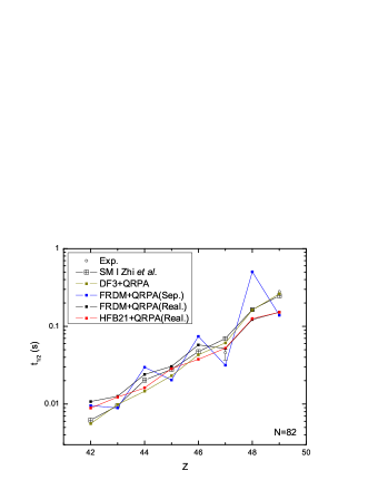
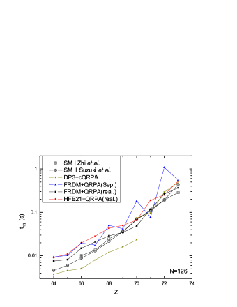
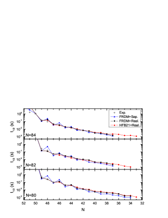
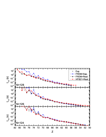
With the determined parameters, we proceed to the calculations of isotonic chains on the r-process path in the vicinity of and . We first show the results with neutron magic number and where the shell model results for these isotones are available. In Figs. 1-3, we show the comparison of our results with shell-model calculations from Ref. SYKO12 ; ZCCLMS13 (SMII resultsSYKO12 are updated by making a correction of a calculations error) and other QRPA calculations such as the QRPA with separable force from Ref. MPK03 and the continuum QRPA from Ref. Bor03 ; Bor11 . For the first-forbidden (FF) part of the decay, Ref. MPK03 uses the gross theory instead of microscopic calculations, while for all the other calculations, the FF parts are calculated explicitly.
We first compare the most important observables – the half-lives predicted by different methods in Fig. 1. For isotones, there is good agreement among different methods except those from separable-force model of Ref. MPK03 for which there are systematic overestimation of half-lives on the even-even isotones compared with other methods for the high Z (low Q) isotones. This is due to their over-estimation of the excitation energies and underestimation of the matrix elements due to the lack of particle-particle interactions for QRPA. This results in an odd-even staggering behaviors for the half-lives in separable-force calculations. However, when the Q becomes large, this effect is reduced as we will see later. Except for Ref. MPK03 , the general discrepancy among different methods for most nuclei is within a factor of two. This shows a good convergence of the predicted half-lives in microscopic calculations. While comparing with the experiments, our method underestimates the half-lives for 131In and 130Cd, especially for the former. The reason for this is that the BCS method does not work well near the doubly-magic nuclei where the pairing is weak and the BCS solution sometimes overestimates the pairing effect as we mentioned previously. For 130Cd the reason for the disagreement is due to the energy of state being too low compared to experiment as seen in Table 1. However, we find better agreement for 129Ag, compared with other methods. The results with FRDM mass model seem agree well with the shell-model calculations while those of the HFB21 mass give a smoother behavior over the isotonic chains. Compared with the shell-model calculation, we find the trend that when Q value becomes larger, our results give some overestimation on the half-lives.
For isotones shown in Fig. 1 the discrepancy between different methods becomes larger. Again, there is a systematic overestimation for results from the separable-force model Ref. MPK03 for even-even nuclei for larger Z. For the continuum-QRPA method, two sets of results are shown; the results from Bor03 systematically underestimate the half-lives, while the results from Ref. Bor11 are closer to other calculations. The two Shell Model calculations give similar results for the half-lives. The difference for the two shell-model calculations comes from the different quenching factors and model space they adopted that produces a nearly small constant difference within a factor of about two. In our calculations, there is difference of less than a factor of two with the two different mass models. The results with the FRDM masses shows a good agreement with the shell-model calculation while those with HFB21 masses give longer half-lives. For most of the nuclei here, with the FRDM mass model, our results differs with the shell model by a factor less than two. Overall, we find good agreement for the half-lives for the isotones among the different methods except those from Ref. MPK03 at high Z and Ref. Bor03 at low Z.
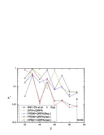
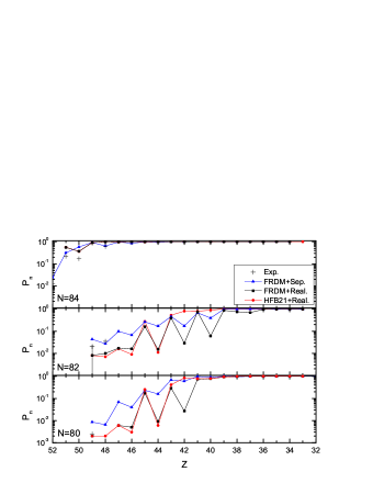
Next we compare the results for the -delayed neutron emission probability in Fig. 2. For the isotones, unlike the half-life results, there are now larger differences among different methods. There is a general trend that the odd-even nuclei have larger values than their neighboring even-even nuclei except results from Ref. Bor03 . We predict lower values than the other calculations, especially for the even-even nuclei. For 130Cd, our result is smaller than the experimental value of 3.5%. In this case the neutrons come from beta decay to the region of excitation in 130In below the beta-decay Q value of 8.9 MeV and above the neutron decay separation energy of 5.1 MeV. Our low value indicates that the QRPA GT distribution in the region of 8 MeV is not spread out enough due to the lack of coupling with particle-hole states. The FRDM+QRPA(Sep.) MPK03 seems to have better predictions for the values, but this comes from the fact that the energy of the lowest state is too high in this case as they predict a much longer half-life for this nucleus, that is, about four times larger than the experimental half-life.
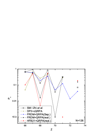
The same situation happens for the isotones (right panel of Fig. 2). The differences among the calculations are quite large for even-even isotones, while there is better agreement for the odd-even cases. In the region , the values are close to . This can be important for the r-process evolution. The shell-model calculation ZCCLMS13 predicts larger values than most other calculations for both and cases, the reason for this is that in shell-model calculations, due to their large configuration space, the strength is fragmented compared with QRPA calculations and more strength has been distributed above the neutron separation energy threshold.
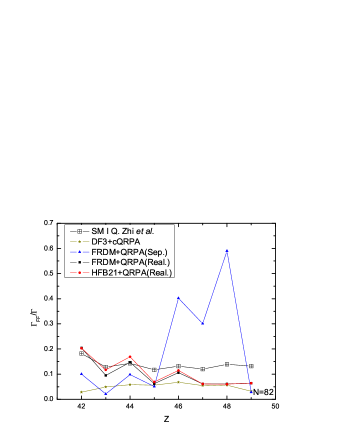
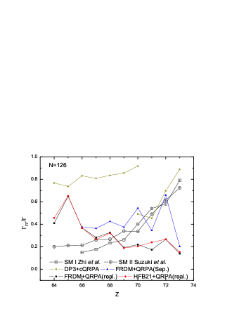
In order to see the importance of inclusion of the first-forbidden part, we compared the ratios of FF part to the overall decay width in Fig. 3. For , except Ref. MPK03 (as they haven’t calculated the FF parts explicitly), the three methods (QRPA, cQRPA and shell model) predict generally similar ratios. We have lower FF ratios which are close to those from cQRPA for high Z and higher FF ratios which are close to shell-model calculations for low Z nuclei. On the other hand, this ratio is about the same for the two mass models in our calculation There is a systematic difference between the cQRPA and shell-model calculations and our results are in between. In general, for the isotonic chain, all the calculations show that the first-forbidden part plays a less important role in -decay. However, this is not the case for the (right panel of Fig. 3) isotonic chain, where there are large discrepancies among different methods. We obtain FF ratios that decrease with Z in contrast to the other methods where they increase. Comparing our results carefully with those of Fig. 16 in Ref.ZCCLMS13 , we found the difference comes from the fact that the two methods have different GT strength distributions. Although the excitation energies for states are similar (around 2 MeV for both methods for three nuclei 194Er,196Yb and 198Hf), the structures of these states are different. In QRPA calculation, we see an small increase of the energies for the first states as the proton number increase, but the energies of the states which give dominant contribution to the GT decay however decrease sharply with the increasing proton number. This is not seen in shell-model calculations. This means that there may be too much strength presented in the low-lying states for N=126 isotones with higher Z due to the configuration space truncations. But on the other hand, shell-model calculations have too limited model space and could result in this different behaviors of GT strength distributions as well. Although Ref. Bor03 has also a very large FF ratio, compared with the same method in Ref. Bor11 , this would be just due to a wrongly accounting of parameters in their calculations and their FF ratios for low Z isotones may need some updates. On the other hand we see that in the two shell-model calculations, the different quenchings and model spaces also give some different ratios as they have similar quenching for the GT part. So as explained above, the difference between our calculation and the shell-model calculations may came from two aspects, the different configuration space and the different model space, and further investigation is needed to explain the discrepancy for the ratios of FF parts.
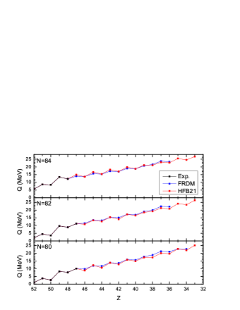
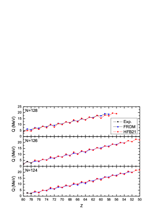
The advantage of QRPA methods is that we can calculate with a larger model space more nuclei than those on the magic number line as in the shell model calculations. So we present more results around the magic number vicinity for even-end nuclei. First, we present the Q value sets we use in our calculation in Fig. 4. As mentioned above, we adopt the Q values if they are available from experimental measurements as those in AWT02 . Otherwise, we use two mass models for the sake of comparison, the FRDM MPK03 mass model come from the macroscopic droplet models and the HFB21 GCP09 model from self-consistent microscopic Hartree-Fock-Boglyubov calculations. From Fig. 4, we see that around the neutron number , the Q-values obtained from the two mass tables are basically the same for most even-even nuclei while there are differences for most odd-even ones, generally FRDM predicts smaller Q-Values except for those nuclei with lower Z. However, for and , the contrary happens and FRDM generally predicts larger Q-values. As for , the same situation happens as for , large difference occurs at low Z. As For and , the discrepancy from the two mass models becomes irregular.
We calculated the half-lives of the isotones with the two mass models and the results are presented in Fig. 5. For 80, 82, 84 isotones, we make comparison with those results in Ref. MPK03 as well as some experimental values. When compared with the experimental results, we find very good agreement. In general, the agreement gets better when the nuclei are far away from the proton magic number . The results with and 84 has the same trends as N=82 we analyzed previously. Compared with results obtained in Ref. MPK03 , we would see the same behaviour of overestimation of even-even nuclei in their calculation with moderate Q values. When the Q value increases the results in both calculations get closer and for much larger Q values, Ref.MPK03 predicts shorter half-lives than ours. The reason for this is due to the different treatments of the excitation energies. In Ref. MPK03 , QRPA energies have been used directly as the excitation energies, which are in fact about several MeV higher than the actual excitation energies. Although the strength spreading has been introduced, even without the quenching effect, the deviation is still large. If Q values are large, then the effect from this difference between QRPA and excitation energies is weakened. Meanwhile the quenching reduces our decay strength and make our predicted half-lives longer than theirs. While in the case of odd nuclei, the single particle transition may play dominant role for low-lying states, we would not see this large deviation of half-lives for isotones with large proton numbers (Z). Generally, for low Q values, deviation occurs for even-even nuclei and agreement is achieved for odd-even nuclei, and for large Q values, we have longer half-lives due to the inclusion of quenching. If we compare the results obtained for the two mass models, we see that for the same nuclei, large Q value shortens the half-life. However, exceptions do exist as the mass model also affect the empirical gap parameters and hence change the structure indirectly. Such as the case of 132Cd, with the same Q value we have a small difference with two mass sets due to the different gap parameters we obtained. Different mass sets produce different half-lives and their impact on r-process is to be investigated. Also, the smoothing behavior of the half-lives on the proton number Z depends on the mass set one chooses. A choice of mass sets may produce the unwanted even-odd staggering behavior. It is somehow hard to tell, whether the staggering comes from the microscopic approaches or the Q value sets, due to the uncertainty of the theory. The same conclusion can be drawn on , 126, 128. One has only limited experimental data in this region, and the agreement for these limited data with the calculations are very poor, as the Q values for these nuclei are very small. For 124 and 126, with the increasing Q values, our calculation tends to agree with calculations of Ref. MPK03 for odd mass nuclei, but for N=128, the deviations always exist. In general, the different mass sets produce a deviation less than a factor of two close to the deviations produced from different methods we discussed for N=126 isotonic chain.
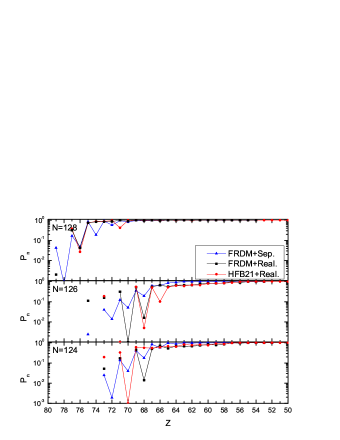
As for another measurable , we have even less experimental data for comparison. Our calculation has smaller values compared with experiments, but the deviation is not large especially when is close to . For and 82, the values increase as the decrease of proton numbers. For very neutron-rich nuclei, the beta-decay is followed immediately with neutron emissions. We see an odd-even staggering behavior as previously found in shell-model calculations. The deviation between our results and those from Ref MPK03 is large in magnitude but keeps the same trends (the reason of this has been explained above as the strength has been shifted to high-energies region systematically in their calculations). However, the two sets of results seem to agree with each other when . This is because the neutron separation energies here are pretty smaller, nearly all the strength lies in the window between and Q. When one crosses the magic number line , there appear increased values as the nuclei here become less stable against the neutron emission, which agrees with results in Ref. MPK03 . For the heavier nuclei region with N around 126, the neutron emission probability hasn’t been measured for any nuclei. The general trends here for the two calculations again keeps the same while they differ in numbers as above. The nuclei beyond the neutron magic number show the large values as for the region of .
Due to the drawbacks of the QRPA methods, limited accuracy has been obtained especially for values. But one could see some improvements of the QRPA calculations, the half-lives are closer to the experimental values as well as those by shell model calculations compared with results inMPK03 . For regions where shell-model calculations are absent, the decent results have been obtained. To further improve the predicted values, the strength spreading from multi-phonon effect could be introduced such as those from the particle-vibration couplings LR06 ; CSB10 .
V conclusion
In this work, we calculated the weak decay properties of even proton number isotones near the neutron magic numbers 82 and 126 with the spherical QRPA method with realistic forces. Our results agree well with other calculations on the neutron magic number chains 82 and 126. We give the predictions for more nuclei in these region and compared with results in Ref. MPK03 . Different mass models have been used for the sake of comparison, and they produce a moderate difference for the final results. In general, we make some improvements on the accuracy of decay rates compared with Ref. MPK03 and its impact on the r-process simulations are to be investigated.
This work was supported by the US NSF [PHY-0822648 and PHY-1068217].
References
- (1) S. E. Woosley, A. Heger and T. A. Weaver, Rev. Mod. Phys. 74, 1015 (2002).
- (2) J. J. Cowan, F. -K. Thielemann and J. W. Truran, Phys. Rept. 208, 267 (1991).
- (3) K. Farouqi, K. -L. Kratz, L. I. Mashonkina, B. Pfeiffer, J. J. Cowan, F. -K. Thielemann and J. W. Truran, Astrophys. J. 694, L49 (2009) [arXiv:0901.2541 [astro-ph.SR]].
- (4) K. Farouqi, K. -L. Kratz, B. Pfeiffer, T. Rauscher, F. -K. Thilemann and J. W. Truran, Astrophys. J. 712, 1359 (2010) [arXiv:1002.2346 [astro-ph.SR]].
- (5) D. -L. Fang, B. A. Brown and T. Suzuki, arXiv:1211.6070 [nucl-th].
- (6) G. Martinez-Pinedo and K. Langanke, Phys. Rev. Lett. 83, 4502 (1999) [astro-ph/9907274].
- (7) K. Langanke and G. Martinez-Pinedo, Rev. Mod. Phys. 75, 819 (2003) [nucl-th/0203071].
- (8) B. A. Brown, Phys. Rev. C 58, 220 (1998).
- (9) T. Suzuki, T. Yoshida, T. Kajino and T. Otsuka, Phys. Rev. C 85, 015802 (2012) [arXiv:1110.3886 [nucl-th]].
- (10) J. J. Cuenca-Garcia, G. Martinez-Pinedo, K. Langanke, F. Nowacki and I. N. Borzov, Eur. Phys. J. A 34, 99 (2007) [arXiv:0811.1189 [astro-ph]].
- (11) Q. Zhi, E. Caurier, J. J. Cuenca-Garcia, K. Langanke, G. Martinez-Pinedo, K. Sieja, arXiv:1301.5225 [nucl-th].
- (12) P. Moller and J. Randrup, Nucl. Phys. A 514, 1 (1990).
- (13) P. Moller, B. Pfeiffer and K. -L. Kratz, Phys. Rev. C 67, 055802 (2003).
- (14) H. Homma, E. Bender, M. Hirsch, K. Muto, H. V. Klapdor-Kleingrothaus and T. Oda, Phys. Rev. C 54, 2972 (1996).
- (15) J. Engel, M. Bender, J. Dobaczewski, W. Nazarewicz and R. Surman, Phys. Rev. C 60, 014302 (1999) [nucl-th/9902059].
- (16) I. N. Borzov and S. Goriely, Phys. Rev. C 62, 035501 (2000).
- (17) I. N. Borzov, Phys. Rev. C 67, 025802 (2003).
- (18) I. N. Borzov, Phys. Atom. Nuvl. 74, 1435 (2011).
- (19) J. Suhonen, T. Taigel and A. Faessler, Nucl. Phys. A486, 91(1988)
- (20) O. Civitarese, A. Faessler and T. Tomoda, Phys. Lett. B 194, 11 (1987).
- (21) H. Behhrens and W. Bühring, Electron Radial Wave Functions and Nuclear Beta Decay(Clarendon, Oxford, 1982).
- (22) R. Machleidt, Adv. Nucl. Phys. 19, 189 (1989).
- (23) B. A. Brown and B. H. Wildenthal, Ann. Rev. of Nucl. Part. Sci. 38, 29 (1988).
- (24) G. Martinez-Pinedo, A. Poves, E. Caurier, and A. P. Zuker, Phys. Rev. C 53, R2602 (1996).
- (25) A. Arima, K. Schimizu, W. Bentz and H. Hyuga, Adv. Nucl. Phys. 18, 1 (1987).
- (26) I. S. Towner, Phys. Rep. 155, 264 (1987).
- (27) G. Audi and A. H. .Wapstra, Nucl. Phys. A729,337(2003).
- (28) G. Audi, A. H. Wapstra and C. Thibault, Nucl. Phys. A 729, 337 (2002).
- (29) S. Goriely, N. Chamel and J. M. Pearson, Phys. Rev. Lett. 102, 152503 (2009) [arXiv:0906.2607 [nucl-th]].
- (30) National Nuclear Data Center [http://www.nndc.bnl.gov/chart/].
- (31) I. Dillmann, K. -L. Kratz, A. Wohr, O. Arndt, B. A. Brown, P. Hoff, M. Hjorth-Jensen and U. Koster et al., Phys. Rev. Lett. 91, 162503 (2003).
- (32) E. K. Warburton, Phys. Rev. C 44, 233 (1991).
- (33) E. Litvinova and P. Ring, Phys. Rev. C 73, 044328 (2006) [nucl-th/0605060].
- (34) G. Colo, H. Sagawa and P. F. Bortignon, Phys. Rev. C 82, 064307 (2010).