Gammalike mass distributions and mass fluctuations in conserved-mass transport processes

Abstract

We show that, in conserved-mass transport processes, the steady-state distribution of mass in a subsystem is uniquely determined from the functional dependence of variance of the subsystem mass on its mean, provided that joint mass distribution of subsystems is factorized in the thermodynamic limit. The factorization condition is not too restrictive as it would hold in systems with short-ranged spatial correlations. To demonstrate the result, we revisit a broad class of mass transport models and its generic variants, and show that the variance of subsystem mass in these models is proportional to square of its mean. This particular functional form of the variance constrains the subsystem mass distribution to be a gamma distribution irrespective of the dynamical rules.

Introduction. – Understanding fluctuations is fundamental to the formulation of statistical mechanics. Unlike in equilibrium, where fluctuations are obtained from the Boltzmann distribution, there is no unified principle to characterize fluctuations in nonequilibrium. In this Letter, we provide a statistical mechanics framework to characterize steady-state mass fluctuations in conserved-mass transport processes.

Nonequilibrium processes of mass transport which happen through fragmentation, diffusion and coalescence are ubiquitous in nature, e.g., in clouds Friedlander , fluids condensing on cold surfaces Meakin , suspensions of colloid-particles White , polymer gels Ziff , etc. To study these processes, various models with discrete as well as continuous time dynamics have been proposed on a lattice where total mass is conserved TakayasuPRL1989 ; MajumdarPRL1998 ; KrugGarcia2000 ; RajeshMajumdar2000 ; Zia_etal_JPhysA2004 ; Evans_JPhysA2005 ; Evans_PRL2006 ; Zielen_JSP2002 ; Zielen_JSP2003 ; Mohanty_JSTAT2012 . These models, a paradigm in nonequilibrium statistical mechanics, are relevant not only for transport of mass, but can also describe seemingly different nonequilibrium phenomena, as diverse as dynamics of driven interacting particles on a ring KrugGarcia2000 , force fluctuations in granular beads Majumdar_Science1995 ; Majumdar_PRE1996 , distribution of wealth Yakovenko ; Patriarca_EPJB2010 , energy transport in solids KMP1982 , traffic flow Krauss1996 ; Chowdhury2000 , and river network Scheidegger , etc.

A striking common feature in many of these processes is that the probability distributions of mass at a single site are described by gamma distributions Majumdar_PRE1996 ; KrugGarcia2000 ; RajeshMajumdar2000 ; Zielen_JSP2002 ; Zielen_JSP2003 ; Mohanty_JSTAT2012 . In several other cases, e.g., in cases of wealth distribution in a population Yakovenko ; Patriarca_EPJB2010 ; AnirbanC or force distribution in granular beads Majumdar_Science1995 ; Majumdar_PRE1996 , the distribution functions are not always exactly known, but remarkably they can often be well approximated by gamma distributions. Although these models have been studied intensively in the past decades, an intriguing question Bertin_PRL2004 - why the gamma-like distributions arise in different contexts irrespective of different dynamical rules - still remains unanswered.

In this Letter, we address these issues in general and explain in particular why mass-transport processes often exhibit gamma-like distributions. Our main result is that, in the thermodynamic limit, the functional dependence of variance of subsystem mass on its mean uniquely determines the probability distribution of the subsystem mass, provided that (i) total mass is conserved and (ii) the joint probability distribution of masses in subsystems has a factorized form as given in Eq. 2. In other words, if the conditions (i) and (ii) are satisfied, the probability distribution $P_{v}(m)$ of mass $m$ in a subsystem of size $v$ can be determined from the functional form of the variance $\sigma_{v}^{2}\equiv\psi(\langle m\rangle)$ where $\langle m\rangle$ the mean. In fact, $\psi(\langle m\rangle)$ in systems with short-ranged spatial correlations can be calculated by integrating two-point spatial correlation function. An important consequence of the main result is the following. When the variance of subsystem mass is proportional to the square of its mean, i.e., $\psi(\langle m\rangle)={\langle m\rangle^{2}}/{v\eta}$ with a parameter $\eta$ that depends on the dynamical rules of a particular model, the subsystem mass distribution is a gamma distribution,

$$P_{v}(m)=\frac{1}{\Gamma(v\eta)}\left(\frac{v\eta}{\langle m\rangle}\right)^{v\eta}m^{v\eta-1}e^{-v\eta m/\langle m\rangle},$$ (1)

where $\Gamma(\eta)=\int_{0}^{\infty}m^{\eta-1}\exp(-m)dm$ the gamma function. Indeed, we find that $\psi(\langle m\rangle)$ is proportional to ${\langle m\rangle^{2}}$ in a broad class of mass-transport models, which explains why these models exhibit gamma distributions.

It might be surprising how the variance alone could determine the probability distribution $P_{v}(m)$ as an analytic probability distribution function is uniquely determined only if all its moments are provided. However, the result can be understood from the fact that, for a system satisfying the above conditions (i) and (ii), there exists an equilibrium-like chemical potential and consequently a fluctuation-response relation that relates mass fluctuation to the response due to a change in chemical potential. This relation, analogous to equilibrium fluctuation-dissipation theorem, provides a unique functional dependence of the chemical potential on mean mass and constrains $P_{v}(m)$ to take a specific form.

Proof. – Let us consider a mass-transport process on a lattice of $V$ sites with continuous mass variables $m_{i}\geq 0$ at site $i=1,\dots,V$. With some specified rates, masses get fragmented and then the neighboring fragments of mass coalesce with each other. At this stage, we need not specify details of the dynamical rules, only assume that the total mass $M=\sum_{i=1}^{V}m_{i}$ is conserved. We partition the system into $\nu$ subsystems of equal sizes $v=V/\nu$ and consider fluctuation of mass $M_{k}$ in $k$th subsystem. We assume that the joint probability ${\cal P}(\{M_{k}\})$ of subsystems having masses $\{M_{1},M_{2},\dots M_{\nu}\}\equiv\{M_{k}\}$ has a factorized form in steady state,

$${\cal P}(\{M_{k}\})=\frac{\prod_{k=1}^{\nu}w(M_{k})}{Z(M,V)}\delta\left({\sum_{k=1}^{\nu}M_{k}-M}\right)$$ (2)

where weight factor $w(M_{k})$ depends only on mass $M_{k}$ of $k$th subsystem and $Z(M,V)=Z(M,v\nu)=\prod_{k=1}^{\nu}[\int dM_{k}w(M_{k})]\delta({\sum_{k=1}^{\nu}M_{k}-M})$ the partition sum.

Probability distribution $P_{v}(m)$ of mass $M_{k}=m$ in the $k$th subsystem of size $v$ is obtained by summing over all other subsystems $k^{\prime}\neq k$, i.e.,

$$P_{v}(m)=\frac{{w(m)}}{Z(M,V)}{\tiny\prod_{k^{\prime}\neq k}\left[\int dM_{k^{\prime}}w(M_{k^{\prime}})\right]\delta\left({\sum_{k}M_{k}-M}\right)}.$$

After expanding $Z(M-m,V-v)$ in leading order of $m$ and taking thermodynamic limit $M,V\gg 1$ with mass density $\rho=M/V$ fixed, we get

$$P_{v}(m)=w(m)\frac{Z(M-m,V-v)}{Z(M,V)}=\frac{w(m)e^{\mu(\rho)m}}{{\cal Z}(\mu)},$$ (3)

where ${\cal Z}(\mu)=\int_{0}^{\infty}w(m)\exp(\mu m)dm$ and chemical potential

$$\mu(\rho)=\frac{df(\rho)}{d\rho}$$ (4)

with $Z(M,V)=\exp[-Vf(\rho)]$ Zia_etal_JPhysA2004 ; Zielen_JSP2002 ; BertinPRE2007 ; PradhanPRE2011 . Using two equalities for mean of the subsystem mass $\langle m\rangle=v\rho=\partial\ln{\cal Z}/\partial\mu$ and its variance $\sigma_{v}^{2}(\langle m\rangle)=(\langle m^{2}\rangle-\langle m\rangle^{2})=\partial^{2}\ln{\cal Z}/\partial\mu^{2}$, a fluctuation-response relation is obtained

$$\frac{d\langle m\rangle}{d\mu}=\sigma_{v}^{2}(\langle m\rangle).$$ (5)

For a homogeneous system, the mean and the variance should be independent of $i$. Moreover, when mass is conserved, the variance is a function of mean mass $\langle m\rangle$ or equivalently density $\rho$. The analogy between Eq. 5 and the fluctuation-dissipation theorem in equilibrium is now evident. Now Eqs. 4 and 5 can be integrated to obtain $Z(M,V)=\exp(-Vf(\rho))$ and then its Laplace transform $\tilde{Z}(s,V)=\int_{0}^{\infty}Z(M,V)e^{-sM}dM.$ Since $[\tilde{Z}(s,V)]^{1/\nu}=\tilde{w}(s),$ the Laplace transform of $w(m),$ one can calculate $w(m)$ straightforwardly and use it in Eq. 3 to get $P_{v}(m)$.

We demonstrate this procedure explicitly in a specific case where the variance of mass in a subsystem of size $v$ is proportional to the square of its mean, i.e.,

$$\sigma_{v}^{2}(\langle m\rangle)\equiv\psi(\langle m\rangle)=\frac{\langle m\rangle^{2}}{v\eta},$$ (6)

with $\eta$ a constant depending on parameters of a particular model. By integrating Eq. 5 w.r.t. $\langle m\rangle=v\rho$ and using Eq. 4 we get

$$\mu(\rho)=-\frac{\eta}{\rho}-\alpha~{}{\rm;}~{}f(\rho)=-\eta\ln\rho-\alpha\rho-\beta.$$ (7)

The integration constants $\alpha$ and $\beta$ do not appear in the final expression of mass distribution. Finally, we get the partition sum $Z(M,V)=\exp[-Vf(\rho)]=({M}/{V})^{\eta V}\exp{(\alpha M+\beta V)}.$ Its Laplace transform $\tilde{Z}(s,V)={e^{\beta V}\Gamma(\eta V+1)}/{[V^{\eta V}(s-\alpha)^{{}^{(\eta V+1)}}]}$ can be written as

$$\tilde{Z}(s,V)\simeq\frac{e^{\beta V}\sqrt{2\pi\eta V}(\eta V)^{\eta V}e^{-\eta V}}{V^{\eta V}(s-\alpha)^{{}^{(\eta V+1)}}}=\frac{\rm{const.}}{(s-\alpha)^{{}^{(\eta V+1)}}}$$ (8)

using asymptotic form of the gamma function $\Gamma(z+1)\simeq\sqrt{2\pi z}z^{z}e^{-z}$ for large $z$. The constant term in the numerator is independent of $s$ and thus $[\tilde{Z}(s,v\nu)]^{1/\nu}$ gives

$$\tilde{w}(s)=\frac{\rm{const.}}{(s-\alpha)^{{}^{v\eta}}}$$ (9)

in the thermodynamic limit $\nu\rightarrow\infty.$ Consequently its inverse Laplace transform is $w(m)\propto m^{v\eta-1}e^{\alpha m}.$ The weight factor $w(m),$ along with Eqs. 3 and 7, leads to $P_{v}(m)$ which is a gamma distribution as in Eq. 1. This completes the proof for the functional form $\psi(x)\propto x^{2}.$ The proof follows straightforwardly for discrete-mass models. Note that different classes of mass distributions $P_{v}(m)$ can be generated for other functional forms of $\psi(x)$ (see Supplemental Material, section I). In all these cases, $P_{v}(m)$ serves as the large deviation function for mass in a large subsystem.

Though the above proof relies on the strict factorization condition Eq. 2, the results are not that restrictive and are applicable to systems when the joint subsystem mass distribution is nearly factorized. In fact, the near-factorization of the joint mass distribution can be realized in a wide class of systems as long as correlation length $\xi$ is finite, i.e., spatial correlations are not long-ranged. In that case, subsystems of size much larger than $\xi$ can be considered statistically independent and thus well described by Eq. 2 Lebowitz_JStatPhys1996 ; BertinPRL2006 ; PradhanPRL2010 .

Models and Discussions. – We now illustrate the results in the context of a broad class of mass-transport models where exact or near factorization condition holds. First we consider driven lattice gases (DLG) on a one dimensional ($1D$) periodic lattice of $L$ sites with discrete masses or number of particles $m_{i}\in(0,1,2,\dots)$ at site $i$ where the total mass $M$ is conserved. A particle hops only to its right nearest neighbor with rate $u(m_{i-1},m_{i},m_{i+1})$ which depends on the masses at departure site $i$ and its nearest neighbors. For a specific rate $u(m_{i-1},m_{i},m_{i+1})={g(m_{i-1},m_{i}-1)g(m_{i}-1,m_{i+1})}/[g(m_{i-1},m_{i})g(m_{i},m_{i+1})],$ the steady-state mass distribution of the model is pair-factorized Evans_PRL2006 , i.e., ${\cal P}(\{m_{i}\})\sim[\prod_{i=1}^{L}g(m_{i},m_{i+1})]\delta(\sum_{i}m_{i}-M)$. Unlike a site-wise factorized state, i.e., Eq. 2 with $\nu=V$, the pair-factorized steady state does generate finite spatial correlations. For a homogeneous function $g(x,y)=\Lambda^{-\delta}g(\Lambda x,\Lambda y),$ the two-point correlation for the rescaled mass $m^{\prime}_{i}=m_{i}/\rho$ can be written as $\langle m^{\prime}_{i}m^{\prime}_{i+r}\rangle\simeq A(r)$ where

$$A(r)=\frac{\prod_{k}\left[\int_{0}^{\infty}dm^{\prime}_{k}g(m^{\prime}_{k},m^{\prime}_{k+1})\right]m^{\prime}_{i}m^{\prime}_{i+r}\delta\left(\sum_{k}m^{\prime}_{k}-L\right)}{\prod_{k}\left[\int_{0}^{\infty}dm^{\prime}_{k}g(m^{\prime}_{k},m^{\prime}_{k+1})\right]\delta\left(\sum_{k}m^{\prime}_{k}-L\right)}$$

is independent of $\rho$. The variance of mass $m=\sum_{i\in v}m_{i}$ in a subsystem of size $v\gg 1$ can be calculated, ignoring small boundary-corrections, as $\sigma^{2}_{v}\simeq v\sum_{r=-\infty}^{\infty}(\langle m_{i}m_{i+r}\rangle-\rho^{2})={\langle m\rangle^{2}}/{\eta v}$ where $\eta^{-1}=\sum_{r=-\infty}^{\infty}[A(r)-1].$ Thus, in DLG with homogeneous $g(x,y)$, $\psi(\langle m\rangle)$ is proportinal to $\langle m\rangle^{2};$ in fact this proportionality is generic in models where steady state is clusterwise factorized with $g$ a homogeneous function of masses at several sites (see Supplemental Material, section II.B). In all these cases, $P_{v}(m)$ should be a gamma distribution.

We now simulate DLG for two specific cases with $g(x,y)=(x^{\delta}+y^{\delta}+cx^{\alpha}y^{\delta-\alpha})$ : Case I. $\delta=1$, $c=0$ and Case II. $\delta=2$, $c=1$ and $\alpha=1.5.$ We then calculate the variance $\sigma^{2}_{v}\equiv\psi(\langle m\rangle)$ as a function of mean mass $\langle m\rangle.$ As shown in Fig. 1(a), in both the cases, $\psi(\langle m\rangle)\propto\langle m\rangle^{2}$ as in Eq. 6 with $\eta\simeq 2.0$ and $\eta\simeq 3.0$ respectively. For these values of $\eta$, corresponding $P_{v}(m)$ obtained from simulations are also in excellent agreement with Eq. 1 as seen in Fig. 1(b). Interestingly, the value of $\eta$ can be calculated analytically for case I where $\delta$ and $\alpha$ are integers (see Supplemental Material, section II.A).

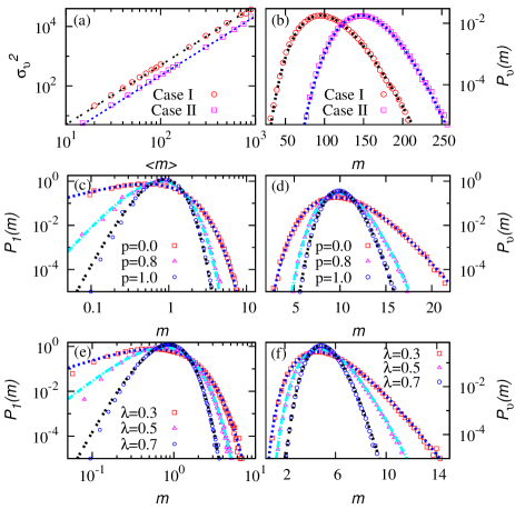
Figure 1: (Color online) Driven lattice gases: (a) Variance $\sigma^{2}_{v}$ of subsystem mass vs. its mean $\langle m\rangle$ (lines - fit to the form in Eq. 6) and (b) corresponding mass distribution $P_{v}(m)$ for Case I. $\delta=1$,$c=0$ and $v=10$ (red circles) and Case II. $\delta=2$, $c=1$, $\alpha=1.5$ and $v=15$ (magenta squares). In both cases $\rho=10$ and $L=2000.$ Mass chipping models: Mass distribution $P_{v}(m)$ vs. mass $m$ with (c) $v=1$ and (d) $v=10$ for the model with $\lambda=1/2$ and $p=0$ (red squares), $0.8$ (magenta triangles) and $1$ (blue circles). Wealth distribution models: Mass distribution $P_{v}(m)$ vs. mass $m$ with (c) $v=1$ and (d) $v=5$ for the model with $\lambda=0.3$ (red squares), $0.5$ (magenta triangles) and $0.7$ (blue circles). In panels (c) - (f), $\rho=1$ and $L=1000$. Simulations - points, gamma distributions (Eq. 1) - dotted lines.

Next we consider a generic variant of paradigmatic mass-transport processes, called mass chipping models (MCM) KrugGarcia2000 ; RajeshMajumdar2000 ; Zielen_JSP2002 ; Zielen_JSP2003 ; Mohanty_JSTAT2012 . These models are based on mass conserving dynamics with linear mixing of masses at neighboring sites which ensures that $\sigma_{v}^{2}\simeq\langle m\rangle^{2}/v\eta$ when the two-point correlations are negligible. Note that, factorizability of steady state necessarily implies vanishing of two-point correlations, but not vice versa. However, when higher order correlations are also small, which is usually the case in these models, the steady state is nearly factorized and the resulting $P_{v}(m)$ can thus be well approximated by gamma distribution for any $v$ (including $v=1$). We demonstrate these results considering mainly the asymmetric mass transfer in MCM; the symmetric case is then discussed briefly.

In $1D,$ asymmetric MCM is defined as follows. On a periodic lattice of $L$ sites with a mass variable $m_{i}\geq 0$ at site $i,$ first $(1-\lambda)$ fraction of mass $m_{i}$ is chipped off, leaving the rest of the mass at $i$. Then a random fraction $r_{i}$ of the chipped-off mass $(1-\lambda)m_{i}$ is transferred to the right nearest neighbor and the rest comes back to site $i$. At each site, the chipping process occurs with probability $p;$ thus the extreme limits $p=0$ and $1$ correspond respectively to random sequential (i.e., continuous-time dynamics) and parallel updates. Effectively, at time $t$, mass $m_{i}(t)$ at site $i$ evolves following a linear mixing-dynamics $m_{i}(t+1)=m_{i}(t)-(1-\lambda)[\gamma_{i}m_{i}(t)-\gamma_{i-1}m_{i-1}(t)],$ where $\gamma_{i}=\delta_{i}r_{i}$ with $\delta_{i}$ and $r_{i}$ are independent random variables drawn at each site $i$ : $\delta_{i}=1$ or $0$ with probabilities $p$ and $1-p$ respectively and $r_{i}$ is distributed according to a probability distribution $\phi(r_{i})$ in $[0,1]$. Ignoring two-point spatial correlations, i.e., taking $\langle m_{i}m_{i-1}\rangle\approx\langle m_{i}\rangle\langle m_{i-1}\rangle=\rho^{2}$, a very good approximation in this case, the variance of mass $\sigma_{1}^{2}=\langle m_{i}^{2}\rangle-\rho^{2}$ at a single site ($v=1$) can be calculated using the stationarity condition $\langle m_{i}^{2}(t+1)\rangle=\langle m_{i}^{2}(t)\rangle$. Then the variance takes a simple form $\sigma_{1}^{2}=\rho^{2}/\eta$ with

$$\eta=\eta(\lambda,p,\mu_{1},\mu_{2})=\frac{\mu_{1}-(1-\lambda)\mu_{2}}{(1-\lambda)(\mu_{2}-p\mu_{1}^{2})}$$ (10)

where $\mu_{k}=\int_{0}^{1}r^{k}\phi(r)dr$ moments of $\phi(r).$ Moreover, in these models, as the two-point correlation function $\langle m_{i}m_{i+r}\rangle-\rho^{2}\simeq 0$ vanishes for $|r|>0$, the variance of subsystem mass is given by $\sigma_{v}^{2}\simeq v\sigma_{1}^{2}=\langle m\rangle^{2}/v\eta.$

A special case of asymmetric MCM with $\lambda=0$ and $p=1$ is the ‘$q$’ model of force fluctuations Majumdar_Science1995 ; Majumdar_PRE1996 which has a factorized steady state for a class of distribution $\phi(r)$ Zielen_JSP2002 . In this case, $P_{1}(m)$ can be immediately obtained by using $\eta={(\mu_{1}-\mu_{2})}/{(\mu_{2}-\mu_{1}^{2})}$ (from Eq. 10) and $v=1$ in Eq. 1. The mass distribution is in perfect agreement with that obtained earlier Zielen_JSP2002 using generating function method. As a specific example, we consider $\phi(r)=r^{a-1}(1-r)^{b-1}/B(a,b)$ with $B(a,b)=\Gamma(a)\Gamma(b)/\Gamma(a+b)$ for which the first two moments are $\mu_{1}=a/(a+b)$ and $\mu_{2}=ab/(a+b)^{2}(a+b+1)-a^{2}/(a+b)^{2},$ and thus $\eta=a+b.$ Corresponding mass distributions is in agreement with that obtained in Zielen_JSP2003 . For $\lambda=0$ and $p<1$, the generalized asymmetric MCM becomes the asymmetric random average process KrugGarcia2000 ; Zielen_JSP2002 ; Zielen_JSP2003 . We consider a specific case, when $r$ is uniformly distributed in $[0,1]$, the steady state is not factorized and exact expression of $P_{1}(m)$ is not known RajeshMajumdar2000 . However, since the two-point correlations vanish RajeshMajumdar2000 , we assume the steady state to be nearly factorized and obtain $P_{1}(m),$ a gamma distribution with $\eta=2/(4-3p).$ We verified numerically that this simple form agrees with the actual $P_{1}(m)$ remarkably well, except for small $m\ll\rho.$

For generic $\lambda$ and $p$ and for a uniform $\phi(r)=1$ with $r\in[0,1]$, the steady state is not factorized Mohanty_JSTAT2012 and the spatial correlations in general are nonzero. Consequently, no closed form expression of the mass distribution is known, except in a mean-field approximation for $\lambda=1/2$ and $p=0$ Mohanty_JSTAT2012 . However, the spatial correlations are small and gamma distribution provides in general a good approximation of $P_{v}(m)$. In Fig. 1(c), $P_{1}(m)$ versus $m$ is plotted for $\lambda=1/2$, $\rho=1$ and for various $p=0,0.8$ and $1$. One can see that $P_{1}(m)$ agrees quite well with Eq. 1 with respective values of $\eta=2$, $5$, and $8$. The deviation for $m\ll\rho$ is an indication of the absence of strict factorization on the single-site level. In Fig. 1(d), distribution $P_{v}(m)$ of mass $m$ in a subsystem of volume $v=10$ is plotted as a function of $m$ and it is in excellent agreement with Eq. 1 almost over five orders of magnitude. Note that, although Eq. 2 does not strictly hold on the single-site level, it holds extremely well for subsystems - a feature observed in MCM or wealth distribution models (discussed later) for generic values of parameters.

In symmetric MCM’s, with parallel update rules, a fraction $\lambda$ of mass $m_{i}$ at site $i$ is retained at the site and fraction $(1-\lambda)$ of the mass is randomly and symmetrically distributed to the two nearest neighbor sites Mohanty_JSTAT2012 : $m_{i}(t+1)=\lambda m_{i}(t)+(1-\lambda)r_{i-1}m_{i-1}(t)+(1-\lambda)(1-r_{i+1})m_{i+1}(t)$ where $r_{i}$ uniformly distributed in $[0,1]$. For $\lambda=0$, the steady state is factorized Mohanty_JSTAT2012 and $P_{1}(m)$ is exactly given by Eq. 1 with $\eta=2$. Clearly, when $\lambda=0$, both symmetric and asymmetric MCM’s with parallel updates result in $\eta=2$, which explains why $P_{1}(m)$ in these two cases are the same Mohanty_JSTAT2012 . Due to the presence of finite spatial correlations, $P_{1}(m)$ with other update rules are not described by Eq. 1.

Our results are also applicable to models of energy transport KMP1982 and wealth distributions Patriarca_EPJB2010 ; Yakovenko ; CCModel ; AnirbanC ; Mohanty_PRE2006 defined on a $1D$ periodic lattice of size $L$. Here, $(1-\lambda)$ fraction of the sum $m^{s}(t)=m_{i}(t)+m_{i+1}(t)$ of individual masses (equivalent to ‘energy’ or ‘wealth’) at nearest-neighbor sites $i$ and $i+1$ is redistributed : $m_{i}(t+dt)=\lambda m_{i}(t)+r(1-\lambda)m^{s}(t)$ and $m_{i+1}(t+dt)=\lambda m_{i+1}(t)+(1-r)(1-\lambda)m^{s}(t)$ where $r$ is uniformly distributed in $[0,1]$. In this process the total mass remains conserved. Assuming $\langle m_{i}m_{i-1}\rangle\approx\rho^{2}$, the variance is written as $\sigma_{1}^{2}(\rho)\approx{\rho^{2}}/{\eta(\lambda)}$ with $\eta(\lambda)={(1+2\lambda)}/{(1-\lambda)}$, in agreement with that found earlier numerically AnirbanC . For $\lambda=0$, i.e., Kipnis-Marchioro-Presutti model in equilibrium KMP1982 , the steady state is factorized and $P_{1}(m)=\exp(-m/\rho)/\rho$ (with $\eta=v=1$) is exact. For non-zero $\lambda$, as the spatial correlations are small, the mass distributions, to a good approximation, are gamma distributions. In Fig. 1(e), $P_{1}(m)$ versus $m$ is plotted for $\lambda=0.3$, $0.5$ and $0.7$ with $\rho=1$ and $L=1000$. Except for $m\ll\rho$, $P_{1}(m)$ agrees well with Eq. 1. For a subsystem of size $v=5$, the distributions $P_{v}(m)$, plotted in Fig. 1(f) for the same parameter values as in the single-site case, are in excellent agreement with Eq. 1 for almost over five orders of magnitude.

Summary. – In this Letter, we argue that subsystem mass fluctuation in driven systems, with mass conserving dynamics and short-ranged spatial correlations, can be characterized from the functional dependence of variance of subsystem mass on its mean. As described in Eq. 2, such systems could effectively be considered as a collection of statistically independent subsystems of sizes much larger than correlation length, ensuring existence of an equilibrium-like chemical potential and consequently a fluctuation-response relation. This relation along with the functional form of the variance, which can be calculated from the knowledge of only two-point spatial correlations, uniquely determines the subsystem mass distribution. We demonstrate the result in a broad class of mass-transport models where the variance of the subsystem mass is shown to be proportional to the square of its mean - consequently the mass distributions are gamma distributions which have been observed in the past in different contexts. From a general perspective, this work could provide valuable insights in formulating a nonequilibrium thermodynamics for driven systems.

Acknowledgment. – SC acknowledges the financial support from the Council of Scientific and Industrial Research, India (09/575(0099)/2012-EMR-I).

References

- (1) S. K. Friedlander, Smoke, Dust and Haze (Wiley Interscience, New York, 1977).
- (2) P. Meakin, Rep. Prog. Phys. 55 157 (1992).
- (3) W. H. White, J. Colloid Interface Sci. 87, 204 (1982).
- (4) R. M. Ziff, J. Stat. Phys. 23, 241 (1980).
- (5) H. Takayasu, Phys. Rev. Lett. 63, 2563 (1989).
- (6) S. N. Majumdar, S. Krishnamurthy, and M. Barma, Phys. Rev. Lett. 81, 3691–3694 (1998).
- (7) J. Krug and J. Garcia, J. Stat. Phys. 99, 31 (2000).
- (8) R. Rajesh and S. N. Majumdar, J. Stat. Phys. 99, 943 (2000).
- (9) M. R. Evans, S. N Majumdar and R K P Zia, J. Phys. A: Math. Gen. 37, L275 (2004).
- (10) M. R. Evans and T. Hanney, J. Phys. A 38, R195 (2005).
- (11) M. R. Evans, T. Hanney, and S. N. Majumdar, Phys. Rev. Lett. 97, 010602 (2006).
- (12) F. Zielen and A. Schadschneider, J. Stat. Phys. 106, 173 (2002).
- (13) F. Zielen and A. Schadschneider, J. Phys. A: Math. Gen. 36, 3709 (2003).
- (14) S. Bondyopadhyay and P. K. Mohanty, J. Stat. Mech. P07019 (2012).
- (15) C.-h. Liu, S. R. Nagel, D. A. Schecter, S. N. Coppersmith, S. N. Majumdar, O. Narayan and T. A. Witten, Science 269, 513 ̵͑(1995͒).
- (16) S. N. Coppersmith, C.-h. Liu, S. N. Majumdar, O. Narayan, and T. A. Witten, Phys. Rev. E 53, 4673 (1996).
- (17) V. M. Yakovenko and J. B. Rosser, Rev. Mod. Phys. 81, 1703 (2009).
- (18) M. Patriarca, E. Heinsalu, and A. Chakraborti, Eur. Phys. J. B 73, 145 (2010).
- (19) C. Kipnis, C. Marchioro, and E. Presutti, J. Stat. Phys. 65, 65 (1982).
- (20) S. Krauss, P. Wagner and C. Gawron, Phys. Rev. E 54, 3707 (1996).
- (21) D. Chowdhury, L. Santen, and A. Schadschneider, Phys. Rep. 329, 199 (2000).
- (22) A. E. Scheidegger, Bull. IASH 12, 15 (1967).
- (23) M. Patriarca, A. Chakraborti, and K. Kaski, Phys. Rev. E 70, 016104 (2004).
- (24) E. Bertin, O. Dauchot, and M. Droz, Phys. Rev. Lett. 93, 230601 (2004).
- (25) G. L. Eyink, J. L. Lebowitz, and H. Spohn, J. Stat. Phys. 83, 385 (1996).
- (26) E. Bertin, O. Dauchot, and M. Droz, Phys. Rev. Lett. 96, 120601 (2006).
- (27) P. Pradhan, C. P. Amann, and U. Seifert, Phys. Rev. Lett. 105, 150601 (2010).
- (28) E. Bertin, K. Martens, O. Dauchot, and M. Droz, Phys. Rev. E 75, 031120 (2007).
- (29) P. Pradhan, R. Ramsperger, and U. Seifert, Phys. Rev. E 84, 041104 (2011).
- (30) A. Chakraborti and B.K. Chakrabarti, Eur. Phys. J. B 17, 167 (2000).
- (31) P. K. Mohanty, Phys. Rev. E 74, 011117 (2006).