Magnon Energy Renormalization and Low-Temperature Thermodynamics of O(3) Heisenberg Ferromagnets

Abstract

We present the perturbation theory for lattice magnon fields of $D$-dimensional O(3) Heisenberg ferromagnet. The effective Hamiltonian for the lattice magnon fields is obtained starting from the effective Lagrangian, with two dominant contributions that describe magnon-magnon interactions identified as a usual gradient term for the unit vector field and a part originating in the Wess-Zumino-Witten term of effective Lagrangian. Feynman diagrams for lattice scalar fields with derivative couplings are introduced, on basis of which we investigate the influence of magnon-magnon interactions on magnon self-energy and ferromagnet free energy. We also comment appearance of spurious terms in the low-temperature series for the free energy by examining magnon-magnon interactions and internal symmetry of the effective Hamiltonian (Lagrangian).

I Introduction

Effective field theory (EFT) is well established method for treating models exhibiting spontaneous symmetry breaking Burgess and is applicable to low-energy part of any system whose only massless excitations are Goldstone bosons AnnPhys . Initially developed for the description of low-energy sector of quantum chromodynamics (QCD), where it is known by the name of the chiral perturbation theory Weinberg ; Gasser ; Gerber ; AnnPhys , EFT was also adapted for the condensed matter problems PRD ; Burgess ; Brauner . In particular, an application of EFT to Heisenberg ferromagnet (HFM) has met with considerable success RomanSoto ; Hofmann1 ; Hofmann2 ; Hofmann3 ; Hofmann4 ; Hofmann5 . As it is well known, the ground state $|0\rangle$ of a HFM is determined by a preferred direction in the internal space, singled out by the total spin $\bm{S}=\sum_{\bm{n}}\bm{S}_{\bm{n}}$ and small fluctuations of the order parameter near the ground state are described by Goldstone bosons (magnons) of spontaneously broken (spin) rotational symmetry. In the low dimensional ($D=1,2$, $D$ being the dimensionality of spatial lattice) isotropic ferromagnets with short-range interactions, rotational symmetry of the Heisenberg Hamiltonian is restored at finite temperatures Mermin and spontaneous symmetry breaking is possible only if $D\geq 3$. (Henceforth we will always assume $D\geq 3$ and nearest neighbor interaction.)

Spontaneous symmetry breaking (SSB) in HFM is distinguished from its Lorentz-invariant counterparts, since the number of Goldstone particles is less than the number of broken generators. In Lorentz-invariant theories, the number of Goldstone bosons ($n_{\text{GB}}$), as well as the number of Goldstone fields ($\pi^{a},\;a=1,2,\dots n_{\text{GB}}$), equals the number of broken symmetry generators ($n_{\text{BS}}$), i.e. $n_{\text{GB}}=n_{\text{BS}}=\mbox{dim}(\mbox{G})-\mbox{dim}(\mbox{H})$. Here G denotes spontaneously broken (internal) symmetry group of the underlying system and H is the symmetry group of the ground state. Even though the symmetry breaking pattern in HFM is $\text{O}(3)\rightarrow\text{O}(2)$, the excitation spectrum contains only one type of magnon. This is related to the fact that ferromagnetic magnons possess nonrelativistic dispersion $\omega\propto\bm{k}^{2}$ due to nonzero vacuum expectation values of charge densities PRD ; PhysLett ; PRDnovi , and a complex field $\psi\propto\pi^{1}+\text{i}\pi^{2}$ describes a single particle Burgess ; PRD ; Hofmann1 ; Hofmann2 ; Hofmann3 ; Hofmann4 ; NielsChad . In other words, $\pi^{1}$ and $\pi^{2}$ represent canonically conjugate variables and not two distinct Goldstone fields Nambu . A general theorem on SSB in Lorentz-noninvariant systems PRDnovi asserts that twice the number $n_{\text{BS}}-n_{\text{GB}}$ equals rank of the matrix $\rho$, defined by its elements $\rho_{ij}=\lim_{V\rightarrow\infty}(-\text{i}/V)\langle 0|[Q_{i},Q_{j}]|0\rangle$, where $V$ denotes the spatial volume of the system and $\{Q_{i}\}$ is the set of broken generators (integrals of charge densities). If, as usual, the spontaneous magnetization aligns in the direction of positive $z$ axis, one finds $\rho\propto\text{diag}[1,-1]$ and corresponding single ferromagnetic magnon. This is in accordance with standard spin-wave theory. The theorem was recently proved in JapanciPRL using EFT (see also related work in PhysLett ; PRDnovi ; Nambu ; JapanciPRL2 ; JapanciPRL3 ; Japanci4 ) demonstrating once again usefulness of the effective Lagrangian method in the theories without Lorentz invariance.

On the other hand, the thermodynamic properties of ferromagnets are usually calculated by some variant of spin-wave theory. The predictions of linear spin-wave theory (LSWT) are reliable almost up to $T_{\text{C}}/2$ ($T_{\text{C}}$ denotes the Curie temperature), but for quantitative description beyond this temperatures one needs to incorporate the effects of magnon-magnon interactions. A successful theory of the spin-wave interactions in Heisenberg ferromagnets was put forward by Dyson Dyson1 ; Dyson2 . He had shown that the kinematical interaction, arising from the limitation on the maximum number ($2S$) of the spin deviations on each lattice site, may safely be ignored at temperatures not to close to $T_{\text{C}}$. Dyson also demonstrated the weakness of dynamical magnon-magnon interaction by calculating first order correction to the free energy and spontaneous magnetization of 3D HFM, thus providing an explanation for the success of LSWT. The weakness of magnon-magnon interactions reflects itself through the changes in the Bloch’s law. The first correction due to magnon-magnon interactions is only of order $T^{4}$, compared to the leading term proportional to $T^{3/2}$. Dyson’s results were subsequently rederived using Holstein-Primakoff bosons Oguchi and the diagram technique for spin operators VLP1 ; VLP2 . (See BKY ; KaganovChubukov ; Borovik ; PSS for a comprehensive reviews and list of original references.) The discovery of high-temperature superconductivity (HTSC) revived interest in the Heisenberg magnets. Since the mid of 1980-ties, a lot of work was put in the understanding of spin-wave interactions in systems of localized spins. Theoretical constructions from this period, dealing explicitly with the Heisenberg ferromagnets, include the modified spin wave theory (MSWT, see Takahasi1 ; Takahasi2 ; Takahasi3 ), the large $N$ expansion of SU($N$) Heisenberg models and Schwinger boson mean field theory (SBMFT, see AuerbachArovas ; SJKM ; Chubukov ), the self-consistent spin wave theory Irkin and renormalization group (RG) methods Kopietz ; Irkin2 . As in the earlier works Oguchi ; VLP1 ; VLP2 ; MBloch , the authors of Takahasi1 ; Takahasi2 ; Takahasi3 ; AuerbachArovas ; SJKM ; Chubukov ; Irkin had shown that a realistic description of the low temperature phase of HFM can be reached using bosonic (or combined bosonic-fermionic Irkin ) representations of the spin operators within quartic approximation, or with the help of appropriate mean field/random phase approximations (MFA/RPA), without complicated mathematical constructions of Dyson. As an alternative to boson/fermion Hamiltonians, obtained from one of many representation of spin operators Garb , several authors developed the method of double time temperature Green’s functions (TGF). (A recent review and original references can be found in Kunc .) It is based on the equations of motion for spin operators, which are turned into a solvable system of algebraic equations by suitable linearization. Known as the decoupling schemes in the language of the double time TGFs, the linearizations incorporate effects of magnon-magnon interactions without any direct reference to the nonlinear boson/fermion Hamiltonian, i.e. to the magnon-magnon interaction operator. One of the most frequently used approximations of this kind is the one by Tyablikov (TRPA, see Kunc ), usually described as the one in which correlations between $S^{z}$ and $S^{\pm}$ operators from adjacent sites are neglected. Magnon energy renormalization, a consequence of Tyablikov’s approximation, affects the low-temperature regime of the theory. The low-temperature expansion of ferromagnetic order parameter for 3D lattice calculated in TRPA contains so called spurious term $\propto T^{3}$, in disagreement with rigorous results of Dyson. Despite this, TRPA yields reliable predictions in accordance with Mermin-Wagner theorem and closed system of equations for correlation functions is often tractable within standard numerical tools. Also, unique solution for critical temperature with self-consistently determined parameters agrees well with Monte Carlo simulations and experimental values Kunc . This aspect of true self-consistency comes to be important when real compounds are modeled by Heisenberg ferromagnet/antiferromagnet (see e.g. PRB ; PRB2 ; SSCCV ; IJMPB ; EPJB ; SSCTNRPA for an application of TRPA to cuprates, iron pnictides and manganites).

The standard theories of non-linear spin waves mentioned in the previous paragraph are based on boson/fermion representations of spin operators. Since the commutation relations for spin operators and the dynamics of the spin system are fully satisfied only with exact boson/fermion Hamiltonian and corresponding Hilbert space, theories of non-linear spin waves are sensitive to any form of approximation. These include, e.g, various mean-field approximations in the Heisenberg spin Hamiltonian VLP1 ; VLP2 ; AuerbachArovas ; SJKM , or approximate boson/fermion expressions for spin operators Oguchi ; Irkin . Similar remark holds for the theories based on the equations of motion for the spin operators where the approximations are made in the commutator for $S^{\pm}$ operators (see Englert ; Stinchcombe and the section II). All these simplifications basically alter the spin nature of $(S^{\pm},S^{z})$ operators in a manner that may not be obvious within a given framework. These problems do not arise in the EFT approach, since one works with true magnon operators from the beginning. All simplifications are directly related to the piece of Lagrangian (Hamiltonian) describing magnon-magnon interactions. This makes the influence of approximation more transparent.

To the best of our knowledge, the perturbation theory with lattice regularization has not yet been applied to the EFT of a ferromagnet. There are several reasons for using a lattice within Hamiltonian formalism. First, unlike dimensional regularization, frequently used within EFT framework AnnPhys ; Hofmann2 ; Hofmann3 ; Hofmann4 ; Hofmann5 , the lattice regularization preserves full discrete symmetry of the original Heisenberg Hamiltonian and it seems to be an appropriate method to deal with system initially defined on a lattice. Second, we will address to some issues inaccessible to the continuum field theoretical methods of Hofmann1 ; Hofmann2 ; Hofmann3 ; Hofmann4 ; Hofmann5 ; PRDnovi ; PhysLett ; NielsChad ; Nambu ; JapanciPRL ; JapanciPRL2 ; JapanciPRL3 ; Japanci4 , such as the influence of interactions on magnon energy renormalization over the entire Brilouin zone. Further, it is the structure of interacting Hamiltonian for ferromagnetic magnons, rather than the general form of interacting Lagrangian, that reveals certain simplifications in the diagrammatic calculation of the magnon self-energy and free energy of O(3) HFM. Although it lacks some of the systematization capabilities of continuum field theoretical approach, the lattice regularized theory can provide us with a useful information not just about spin systems but also on other standard techniques. For example, by examining magnon mass renormalization in sections IV and VI, we reach a clear explanation for spurious $T^{3}$ term in Tyablikov RPA.

The section II contains brief discussion on LSWT, the magnon mass renormalization and its influence on the spontaneous magnetization. Some notation on the lattice theory, such as the lattice Laplacian, are likewise introduced there. The effective interaction Hamiltonian of lattice magnons is derived in the Section III, starting from the effective Lagrangian. The Feynman diagrams with colored propagators and vertices, suitable for theories of lattice scalar fields with derivative couplings are also defined in the Section III. Two-loop perturbation theory for lattice magnon self-energy is presented in the Section IV, while three-loop analysis of the free energy is given in the Section V. Results of Section VI, based on continuum field theoretic calculation supplement and clarify findings of two preceding Sections. An important feature of the effective Hamiltonian is identification of the two types of magnon-magnon interaction different in origin. The careful discussion in sections III–VI offers a new answer for appearance of the spurious terms in the low-temperature series and demonstrates the influence of spin-rotation symmetry on the thermodynamic properties of O(3) HFM. Finally, some calculation details and an alternative formulation of the O(2) model of the Subsection IV.4 are collected in the Appendices.

II Preliminary discussion

In this section we are motivating approach to be discussed in detail latter. Also, for the clarity of presentation, we find it convenient to introduce some notation on lattice fields before general perturbation theory.

First, it is instructive to rewrite the Hamiltonian of Heisenberg ferromagnet with nearest neighbor interaction $J$ on a $D$ dimensional lattice

$$H = -\frac{J}{2}\sum_{\bm{n},\;\bm{\lambda}}\bm{S}_{\bm{n}}\cdot\bm{S}_{\bm{n}+\bm{\lambda}},$$ (1)

in terms of the discrete Laplacian

$$H = -\frac{1}{2}\;\frac{JZ_{1}|\bm{\lambda}|^{2}}{2D}\sum_{\bm{x}}\bm{S}_{\bm{x}}\cdot\nabla^{2}\bm{S}_{\bm{x}}-\frac{JS(S+1)Z_{1}N}{2}.$$ (2)

Here $[S_{\bm{x}}^{i},S_{\bm{y}}^{j}]=\text{i}\epsilon_{ijk}S_{\bm{x}}^{k}\Delta(\bm{x}-\bm{y})$, $\bm{S}^{2}=S(S+1)$, the lattice Laplacian is (See e.g. LatLapl )

$$\nabla^{2}\phi(\bm{x})=\frac{2D}{Z_{1}|\bm{\lambda}|^{2}}\sum_{\bm{\lambda}}\Big{[}\phi(\bm{x}+\bm{\lambda})-\phi(\bm{x})\Big{]},$$ (3)

$\{\bm{\lambda}\}$ are the vectors that connect given site $\bm{x}$ with its $Z_{1}$ nearest neighbors and $N$ is the total number of lattice sites. As we are mainly interested in finite temperatures, imaginary time formalism is used throughout the paper (unless otherwise stated). Employing $-\partial_{\tau}S_{j}(\bm{n},\tau)=[S_{j}(\bm{n},\tau),H],j=1,2,3$, equation of motion for $\bm{S}(\bm{x},\tau)$ is found to be (imaginary time arguments are suppressed)

$$-\partial_{\tau}\bm{S}(\bm{x}) = -\frac{\text{i}}{2}\;\frac{JZ_{1}|\bm{\lambda}|^{2}}{2D}\Big{[}\Big{(}\nabla^{2}\bm{S}(\bm{x})\Big{)}\times\bm{S}(\bm{x})$$ (4)

$$- \bm{S}(\bm{x})\times\nabla^{2}\bm{S}(\bm{x})\Big{]}.$$

Eq. (4) is just the lattice version of imaginary time Landau-Lifshitz equation for operators $\bm{S}(\bm{x},\tau)$. It can be solved in a linear approximation. Assuming the long range order (LRO), we may set $S^{z}(\bm{n})\approx S$  . In this approximation, equation of motion for $S^{+}(\bm{x})=S^{x}(\bm{x})+\text{i}S^{y}(\bm{x})$ takes the form of the imaginary time equation for Schrödinger field on the lattice

$$-\partial_{\tau}S^{+}(\bm{x}) = -\frac{1}{2m_{\text{LSW}}}\nabla^{2}S^{+}(\bm{x}),$$ (5)

where we have defined

$$m_{\text{LSW}}=\frac{2D}{2JSZ_{1}|\bm{\lambda}|^{2}}.$$ (6)

Similar equation holds for $S^{-}(\bm{x})=S^{x}(\bm{x})-\text{i}S^{y}(\bm{x})$. Simultaneously, the linearized commutation relations for $S^{\pm}$ operators read

$$\left[\frac{S^{+}(\bm{x})}{\sqrt{2S}},\frac{S^{-}(\bm{y})}{\sqrt{2S}}\right]=\Delta(\bm{x}-\bm{y}).$$ (7)

Comparing (7) to the usual form of equal-time commutation relations, $[\psi(\bm{x}),\psi^{\dagger}(\bm{y})]=v_{0}^{-1}\Delta(\bm{x}-\bm{y})$, where $v_{0}$ denotes volume of the primitive cell, we see that in this approximation the Heisenberg ferromagnet is described by the bosonic lattice Schrödinger fields

$$\psi(\bm{x},\tau)=\frac{S^{+}(\bm{x},\tau)}{\sqrt{2Sv_{0}}},\;\;\;\;\psi^{\dagger}(\bm{x},\tau)=\frac{S^{-}(\bm{x},\tau)}{\sqrt{2Sv_{0}}},$$ (8)

which annihilate and create magnons at lattice site $\bm{x}$, respectively. Schrödinger field interpretation can be further justified by solving equation (5) and constructing a diagonal Hamiltonian. Finding plane-wave solutions Fetter of (5)

$$\psi(\bm{x},\tau)=\int_{\bm{k}}a_{\bm{k}}\;\text{e}^{\text{i}\bm{k}\cdot\bm{x}-\omega(\bm{k})\tau},\;\;\;\int_{\bm{k}}\equiv\int_{\text{IBZ}}\frac{\text{d}^{D}\bm{k}}{(2\pi)^{D}}$$ (9)

and using eigenvalues of the lattice Laplacian

$$\nabla^{2}\exp[\text{i}\bm{k}\cdot\bm{x}]=-\frac{2D}{|\bm{\lambda}|^{2}}[1-\gamma_{D}(\bm{k})]\exp[\text{i}\bm{k}\cdot\bm{x}]$$

$$\equiv -\widehat{\bm{k}}^{2}\exp[\text{i}\bm{k}\cdot\bm{x}],\;\;\;\;\;\;\gamma_{D}(\bm{k})=Z_{1}^{-1}\sum_{\{\bm{\lambda}\}}\exp[\text{i}\bm{k}\cdot\bm{\lambda}],$$

we find the magnon dispersion

$$\omega_{\text{LSW}}(\bm{k}) = \frac{\widehat{\bm{k}}^{2}}{2m_{\text{LSW}}}=JZ_{1}S[1-\gamma_{D}(\bm{k})],$$ (11)

and diagonal magnon Hamiltonian in the linear approximation

$$H_{0} = -\frac{v_{0}}{2m_{\text{LSW}}}\sum_{\bm{x}}\psi^{\dagger}(\bm{x})\nabla^{2}\psi(\bm{x})-E_{0}$$

$$= V\int_{\bm{k}}\omega_{\text{LSW}}(\bm{k})\;n_{\bm{k}}-E_{0},\;\;\;E_{0}=\frac{JZ_{1}NS^{2}}{2},$$

where $Vn_{\bm{k}}=a_{\bm{k}}^{\dagger}a_{\bm{k}}$ and $V=(2\pi)^{D}\delta(\bm{k}-\bm{k})=Nv_{0}$. $a_{\bm{k}}$ and $a_{\bm{k}}^{\dagger}$ are standard bosonic operators obeying commutation relations $[a_{\bm{k}},a_{\bm{q}}^{\dagger}]=(2\pi)^{D}\delta(\bm{k}-\bm{q})$. Operating on the vacuum $|0\rangle$, $a_{\bm{p}}^{\dagger}$ creates one-magnon state $a_{\bm{p}}^{\dagger}|0\rangle=|\bm{p}\rangle$. These states are normalized as $\langle\bm{p}|\bm{q}\rangle=(2\pi)^{D}\delta(\bm{p}-\bm{q})$ PRD . We may now identify $m_{\text{LSW}}$ as (bare) mass of the lattice field quanta i. e. magnons. We shall continue to refer to $m_{\text{LSW}}$ as a magnon mass because of the nonrelativistic form of the dispersion relation (11), even though ferromagnetic magnons are ”massless” from the point of view of the Goldstone theorem.

The diagonal Hamiltonian makes thermodynamical properties of a ferromagnet trivial to calculate. For example, at low temperatures, the spontaneous magnetization per lattice site is found to be a vacuum expectation value of

$$S_{\bm{x}}^{z} = \sqrt{S(S+1)-[S^{x}_{\bm{x}}]^{2}-[S^{y}_{\bm{x}}]^{2}}\approx S-\frac{S_{\bm{x}}^{-}S_{\bm{x}}^{+}}{2S}$$ (13)

$$= S-v_{0}\psi^{\dagger}(\bm{x})\psi(\bm{x}).$$

Written in terms of the thermal propagator for Schrödinger field

$$D(\bm{x}-\bm{y},\tau_{x}-\tau_{y}) = \langle\mbox{T}\left\{\psi(\bm{x},\tau_{x})\psi^{\dagger}(\bm{y},\tau_{y})\right\}\rangle_{0}$$

$$= \frac{1}{\beta}\sum_{n=-\infty}^{\infty}\int_{\bm{q}}\frac{\text{e}^{\text{i}\bm{q}\cdot(\bm{x}-\bm{y})-\text{i}\omega_{n}(\tau_{x}-\tau_{y})}}{\omega(\bm{k})-\text{i}\omega_{n}},$$

it is

$$\langle S^{z}\rangle=S-v_{0}\int_{\bm{q}}\langle n_{\bm{q}}\rangle_{0}=S-v_{0}D(0).$$ (15)

Here $D(0)$ denotes the propagator evaluated at the origin, $\langle n_{\bm{q}}\rangle_{0}$ is the free-magnon Bose distribution and we have used the sum rule Fetter $\beta^{-1}\sum_{n}[\omega_{0}({\bm{p}})-\text{i}\omega_{n}]^{-1}=\langle n_{\bm{p}}\rangle_{0}$. Results (6)-(II), which define the lattice theory of free Schrödinger field, are easily seen to be those of standard linear spin waves (LSW).

The question of how to incorporate the effects of magnon-magnon interactions into equations like (15) has long history and long list of answers. They are grouped in several categories as described in the Introduction. The primary goal of the present paper is to show that thermodynamic properties of a $D$ dimensional O(3) Heisenberg ferromagnet may be calculated within formalism of interacting lattice Schrödinger field, based on the effective Lagrangian. We will show, e.g., that the spontaneous magnetization of O(3) HFM to the first order in $1/S$, can be written as $S-v_{0}G(0)$, where $G(0)$ is the magnon field Green’s function calculated to the one loop. Also, in Sections III–VI we develop the perturbation theory capable for calculating both micro and macro properties of O(3) HFM.

Returning to the magnon dispersion, it is easily seen that approximation $S^{z}(\bm{n})\approx\langle S^{z}\rangle$ in (4) eventually leads to TRPA result with the magnon energies

$$\omega_{\text{RPA}}(\bm{k}) = \frac{\widehat{\bm{k}}^{2}}{2m_{\text{RPA}}},\;\;\;\;m_{\text{RPA}}=\frac{2D}{2J\langle S^{z}\rangle Z_{1}|\bm{\lambda}|^{2}}.$$ (16)

As happens in LSWT, the final result in TRPA contains no information about the short range fluctuations (SRF) of the order parameter if the operator $S^{z}(\bm{n})$ is replaced with the site independent average $\langle S^{z}\rangle$. (A discussion about the role of SRF can be found in a recent review Plakida .) In spite of that, TRPA incorporates certain type of magnon-magnon interaction that renormalizes magnon mass according to (16). Since the approximation is made directly in the equation of motion, an explicit form of magnon-magnon interactions that yield (16) can’t be deduced in TGF formalism. Tyablikov’s result (16) for HFM was subsequently re-derived by linearizing the commutation relations for Fourier components of $S^{\pm}_{\bm{n}}$ operators Englert ; Stinchcombe similarly as in this section, using the perturbation theory for self-consistent mean field approximation VLP1 ; VLP2 , various diagram techniques for spin operators BKY ; Fishman , drone-fermion for $S=1/2$ and $S=1$ Spencer and pseudofermion representation for spin $S=1/2$ ferromagnets KineziRPA . Although both the spin-operator diagram technique and the pseudo/drone fermion representations eventually yield TRPA result (or improve it), non of these approaches describes HFM as a system of interacting magnons built on LSWT as the non-interacting theory, i.e. using the perturbation theory for interacting magnon fields without additional MFA/RPA approximations. The issue of magnon-magnon interactions in TRPA can be resolved by interpreting TRPA as a certain type of EFT. As a corollary, we will give a clear answer for the spurious $T^{3}$ term of Tyablikov.

III Effective interaction of the lattice magnon fields

We have seen in the previous section that the LSWT description of HFM is equivalent to a theory of free lattice Schrödinger field. The rest of the present paper will be devoted to the influence of magnon-magnon interactions on microscopic and macroscopic properties of a ferromagnet. The simplest choice of the interaction for the Schrödinger field, with the Hamiltonian density $\propto[\psi^{\dagger}(\bm{x})\psi(\bm{x})]^{2}$ simply won’t work because the vertices of $[\psi^{\dagger}(\bm{x})\psi(\bm{x})]^{2}$ interaction carry no momentum, so it can not renormalize the mass of a ferromagnetic magnon. The correct form of the effective interaction is most easily formulated in terms of the Goldstone fields $\pi^{a}(\bm{x})$.

III.1 Effective Lagrangian

As noted in the Introduction, the general effective Lagrangian is written in terms of Goldstone fields $\pi^{a}(x),a=1,2\dots\text{dim(G)}-\text{dim(H)}$. Various terms appearing in the effective Lagrangian are organized in the powers of momenta of the Goldstone fields. The leading order Lagrangian collects all contributions of the order $\bm{p}^{2}$. If the system is invariant under parity, which is the case with the Heisenberg Hamiltonian (1), only terms with even powers of momenta are permitted. The next-to-leading order Lagrangian then contains all contributions of the order $\bm{p}^{4}$ and so on. Translated into the direct space, the powers of momenta correspond to the derivatives. The effective Lagrangian is constructed by adding terms with increasing number of derivatives of the Goldstone fields, with the lowest order term containing two derivatives. It should be noted that for systems whose massless excitations characterize nonrelativistic dispersion $\omega\propto\bm{p}^{2}$, such is HFM, single time derivative counts as $\bm{p}^{2}$, i.e. as two spatial derivatives or a single power of temperature PRD ; Hofmann2 ; Hofmann3 . Expansion in the powers of momentum is always terminated at some finite order and, beside Goldstone fields and their derivatives, the effective Lagrangian also includes several coupling constants whose values are not specified by the symmetry requirements. They can be determined by comparison of predictions of EFT with numerical simulations, experimental results or by matching with detailed microscopic calculations Burgess ; AnnPhys . When the effective Lagrangian is constructed, a straightforward application of Feynmann rules enables one to calculate the correlation functions, partition function etc. For a Heisenberg ferromagnet $\text{G}=\text{O}(3),\text{H}=\text{O}(2)$, and the spontaneous symmetry breaking is accompanied by two real Goldstone fields $\pi^{1}(x)$ and $\pi^{2}(x)$. However, the ferromagnetic magnons possess nonrelativistic dispersion relation ($\omega\propto\bm{k}^{2}$) and a complex field $\psi\propto\pi^{1}+\text{i}\pi^{2}$ describes a single magnon PRD ; Hofmann1 ; Hofmann2 ; Hofmann3 ; Burgess ; NielsChad ; JapanciPRL ; Nambu .

Effective Lagrangian for HFM was introduced in PRD ; RomanSoto ; Wiese (see also earlier works Jevicki ; Klauder ; WenZee ), and a detailed derivation of the partition function up to the three loops using continuum approximation and the dimensional regularization, resulting with the leading corrections to Dyson’s analysis of 3D HFM, can be found in Hofmann3 (see also Hofmann1 ; Hofmann2 and Hofmann4 ; Hofmann5 for corresponding analysis of the two dimensional ferromagnet). In the present paper, a slightly modified path will be followed. As one of our interests lies in the mass renormalization of the lattice magnons, we wish to preserve the full discrete symmetry of lattice spin Hamiltonian (1). Because of that, we find it more convenient to work in the Hamiltonian formulation of lattice field theory Hamer ; Kogut , leaving only (imaginary) time coordinate continuous. Therefore, the first task is to construct the effective Hamiltonian that describes interactions of lattice magons with nonrelativistic dispersion. Details for lattice regularization of the Lorentz-invariant effective field theory can be found e.g. in Smilga ; Lewis .

The leading order real time effective Lagrangian of O(3) ferromagnet is PRD ; Wiese ; Jevicki

$${\mathcal{L}}_{\text{eff}}=\Sigma\frac{\partial_{t}U^{1}U^{2}-\partial_{t}U^{2}U^{1}}{1+U^{3}}-\frac{F^{2}}{2}\partial_{\alpha}U^{i}\partial_{\alpha}U^{i},$$ (17)

where two magnon fields are collected into the unit vector $U^{i}:=[U^{1},U^{2},U^{3}]^{\text{T}}\equiv[\bm{\pi}(x),U^{3}(x)]^{\text{T}}$, $\Sigma=NS/V$ is the spontaneous magnetization per unit volume at $T=0$K and $F$ is a constant. The first part of Lagrangian is usually denoted as Wess-Zumino-Witten (WZW) term. It gives rise to the Berry phase Wen and is responsible for the classical dispersion of the ferromagnetic magnons ($\omega\propto\bm{k}^{2}$). The presence of WZW term makes Lagrangian rotationally invariant only up to the total derivative. As it will be shown, the inclusion of magnon-magnon interactions arising from WZW term is crucial for correct low-temperature description of O(3) HFM. The next-to-leading order Lagrangian contains terms such as $l_{1}(\partial_{\alpha}U^{i}\partial_{\alpha}U^{i})^{2}$, $l_{1}(\partial_{\alpha}U^{i}\partial_{\beta}U^{i})^{2}$, $l_{3}U^{i}\Delta^{2}U^{i}$, or $l_{4}\partial^{2}_{\alpha}U^{i}\partial^{2}_{\alpha}U^{i}$ with arbitrary coupling constants $l_{1},\dots l_{4}$ Hofmann2 ; Hofmann3 . These ${\mathcal{O}}(\bm{p}^{4})$ terms shall not be directly included in the effective Hamiltonian. Instead, higher order momentum contributions will appear naturally in a lattice regularized theory. This regularization, however, restricts possible choices for higher order terms (See section VI).

III.2 Transition to interaction picture

The use of perturbation theory requires clear separation between the free-magnon part, which must be identified with (II), and the interaction part of the Hamiltonian WeinbergQTF1 . To extract them from the Lagrangian (17), we may rewrite it in terms of the complex field $\psi=\sqrt{\Sigma/2}[\pi^{1}+\text{i}\pi^{2}]$ which describes the physical magnon, and follow the standard canonical prescription. However, this is not the most efficient way to construct interaction picture. The WZW term modifies canonical momentum, from $\text{i}\psi^{\dagger}$ of noninteracting theory, to $2\text{i}\psi^{\dagger}/[1+U^{3}]$, where $U^{3}=\sqrt{1-(2/\Sigma)\psi^{\dagger}\psi}$. Consequently, the complex fields $\psi$ and $\psi^{\dagger}$ that enter Hamiltonian are not those obeying equal-time commutation relations. As the connection between canonical momentum and $\psi^{\dagger}$ is highly nonlinear it can be solved for $\psi^{\dagger}$ only iteratively. Because of that, an important part of magnon-magnon interactions is not manifest in the Hamiltonian, since it enters the quantum theory through the failure of $\psi$ and $\psi^{\dagger}$ to satisfy canonical Schrödinger-field commutation relations. This is reminiscent of the situation dealt with in the spin-operator approach to Heisenberg magnets: the commutation relations governing the dynamics of system are neither Bose nor Fermi type and the interaction is generated by expanding localized spins operators in terms of boson/fermion operators Oguchi ; BKY ; Garb ; Irkin ; Borovik . For the present purposes, however, it is desirable to have an explicit form of the magnon-magnon interaction.

A different strategy WeinbergQTF1 makes use of the equation of motion, which in the present case is the Landau-Lifshitz equation PRD ,

$$\partial_{t}U^{a}+\frac{F^{2}}{\Sigma}\;\varepsilon_{aij}(\Delta U^{i})U^{j}=0,$$ (18)

to eliminate $\dot{\pi}^{1}$ and $\dot{\pi}^{2}$ from the interaction part of the Lagrangian (17). Here $\Delta=\partial_{\alpha}\partial_{\alpha}$. In this manner we find the free-magnon Lagrangian

$${\mathcal{L}}_{\text{free}}=\frac{\Sigma}{2}\left[\partial_{t}\pi^{1}\pi^{2}-\partial_{t}\pi^{2}\pi^{1}\right]+\frac{F^{2}}{2}\bm{\pi}\cdot\Delta\bm{\pi},$$ (19)

and the interaction piece

$${\mathcal{L}}_{\text{int}}=\frac{F^{2}}{2}\left[2-\bm{\pi}^{2}-\sqrt{1-\bm{\pi}^{2}}\right]\Delta\sqrt{1-\bm{\pi}^{2}}-\frac{F^{2}}{2}\frac{1-\sqrt{1-\bm{\pi}^{2}}}{1+\sqrt{1-\bm{\pi}^{2}}}\sqrt{1-\bm{\pi}^{2}}\;\bm{\pi}\cdot\Delta\bm{\pi}.$$ (20)

Canonical interacting quantum theory can now be easily constructed starting from ${\mathcal{L}}_{\text{free}}$ and ${\mathcal{L}}_{\text{int}}$. To perform two-loop calculations for the self-energy ant three-loop calculations for the free energy, we need to retain tjhe magnon-magnon interaction up to and including six magnon operators. By expanding (20) we find that terms with six $\pi^{a}$ operators precisely cancel, in contrast to a Lorentz-invariant theory Gerber ; Smilga . Remaining four-magnon terms are then collected to

$${\mathcal{H}}_{\text{int}}=\frac{F^{2}}{8}\bm{\pi}^{2}\left[\bm{\pi}\cdot\Delta\bm{\pi}-\Delta\bm{\pi}^{2}\right].$$ (21)

Finally, by putting the free Hamiltonian and interaction part (21) on the lattice, we obtain the effective Hamiltonian for lattice magnon fields

$$H_{\text{eff}} = H_{0}+H_{\text{int}},$$ (22)

$$H_{0} = -\frac{1}{2m_{0}}v_{0}\sum_{\bm{x}}\psi^{\dagger}(\bm{x})\nabla^{2}\psi(\bm{x}),\;\;\;m_{0}=\frac{\Sigma}{2F^{2}}$$

$$H_{\text{int}} = \frac{F^{2}}{8}v_{0}\sum_{\bm{x}}\bm{\pi}^{2}(\bm{x})\left[\bm{\pi}(\bm{x})\cdot\nabla^{2}\bm{\pi}(\bm{x})-\nabla^{2}\bm{\pi}^{2}(\bm{x})\right]$$ (23)

$$\equiv H_{\text{int}}^{(\text{I})}+H_{\text{int}}^{(\text{II})},$$

where $\nabla^{2}$ denotes the lattice Laplacian and the lattice Schrödinger field is ($\Sigma=S/v_{0}$ in a lattice theory)

$$\psi(\bm{x})=\sqrt{\frac{S}{2v_{0}}}\left[\pi^{1}(\bm{x})+\text{i}\pi^{2}(\bm{x})\right].$$ (24)

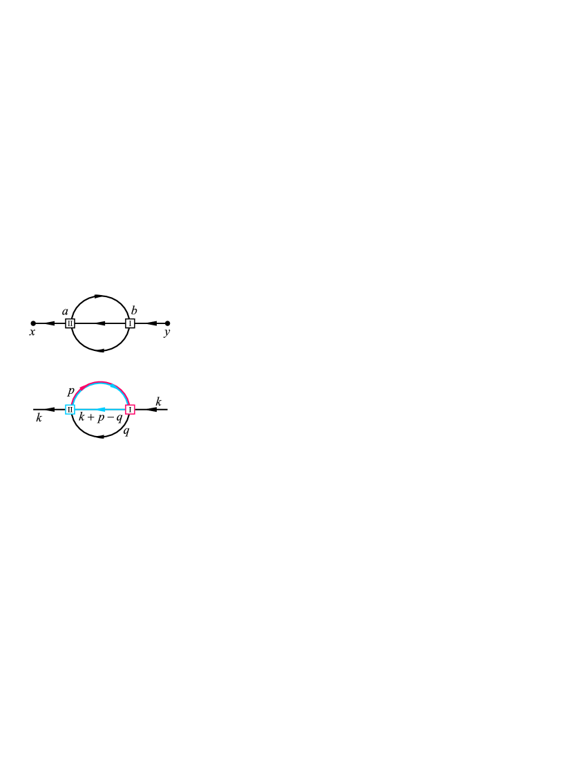
Figure 1: (Color online) Coordinate space representation of a diagram contributing to the self-energy of lattice magnon field (top) and one of its contractions in momentum space (bottom). Vertices from $H_{\text{int}}^{(\text{I})}$ and $H_{\text{int}}^{(\text{II})}$ are denoted by red and blue squares, respectively. The blue line denotes propagator affected by lattice Laplacians of $H_{\text{int}}^{(\text{II})}$. The double colored line represents propagator acted on by Laplacians of both $H_{\text{int}}^{(\text{I})}$ and $H_{\text{int}}^{(\text{II})}$.

In what follows, $\psi$ will always be written to the right in expressions like $\bm{\pi}\cdot\bm{\pi}$. $H_{0}$ is basically LSWT Hamiltonian (II) and with this choice for ${\mathcal{L}}_{\text{free}}$ and ${\mathcal{L}}_{\text{int}}$ (i.e. $H_{0}$ and $H_{\text{int}}$), $\psi$ and $\psi^{\dagger}$ do satisfy canonical commutation relations for Schrödinger field. Unlike in its continuous counterpart, the discrete symmetry of the original Hamiltonian (1) that modifies magnon dispersion in higher orders of momentum is fully preserved in (22) and (23). Hence, all higher order terms in momentum, i.e. in spatial derivatives, that resolve the lattice structure at the same time describing the free magnons are collected in $H_{0}$. This fact simplifies further calculations. Magnon-magnon interactions in accord with lattice structure and internal symmetries, to the order considered here, are collected in $H_{\text{int}}$. One can choose constant $F^{2}$ to be $\Sigma/(2m_{\text{LSW}})=JS^{2}Z_{1}|\bm{\lambda}|^{2}/(2Dv_{0})$, so that the energy of free lattice magnons is measured in units of $J$ , as in LSWT (see (11) and (II)). Of course, this is unnecessary, since the value of $F$ can be deduced from the experimental data on magnon dispersion. In terms of the unit vector $\bm{U}$, spontaneous magnetization can be calculated as $\langle S^{z}\rangle=S\langle U^{3}\rangle\approx S-(S/2)\langle\bm{\pi}^{2}\rangle$, which coincides with (15). Hamiltonian (22) resembles the Hamiltonian first obtained by Dyson, starting from nonorthogonal multi spin-wave states Dyson1 . It was subsequently rederived using boson representations for the spin operators Oguchi ; Maleev . However, (22) is expressed in terms of true magnon field operators, with no direct connection to the localized spins of (1). Also, it is seen from the derivation of (22) that $H_{\text{int}}^{(\text{II})}$ has the form of the usual gradient contribution in the Hamiltonian of a unit vector field, while $H_{\text{int}}^{(\text{I})}$ describes magnon-magnon interactions originating in the WZW term (A part of interactions form WZW-term of the form $\bm{\pi}^{2}\nabla^{2}\bm{\pi}^{2}$ are present in $H_{\text{int}}^{(\text{II})}$ too). athe magnon-magnon interactions collected in $H_{\text{int}}^{(\text{I})}$ are therefore essential for preserving the spin characteristics of bosonic field $\bm{U}(\bm{x})$.

After the free and interaction parts of the Hamiltonian have been constructed, the perturbation theory may be applied to calculate the Green’s function

$$G(\bm{x}-\bm{y},\tau_{x}-\tau_{y})=\frac{\langle\mbox{T}\left\{\psi(\bm{x},\tau_{x})\psi^{\dagger}(\bm{y},\tau_{y})U(\beta)\right\}\rangle_{0}}{\langle U(\beta)\rangle_{0}}$$ (25)

with $U(\beta)=\mbox{T}\exp\left\{-\int_{0}^{\beta}\text{d}\tau H_{\text{int}}(\tau)\right\}$, and the free energy, thereby determining the influence of interaction on magnon energies and thermodynamic properties of the system. By expanding the exponential in definition of $U(\beta)$, we arrive at the Feynman rules for interacting lattice magnon fields in O(3) HFM. We shall now introduce a convenient variant of Feynman diagrams.

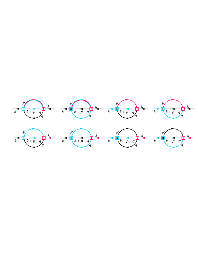
Figure 2: (Color online) All possible momentum-space (colored) contractions corresponding to the upper diagram of FIG 1. Each colored line denotes the lattice Laplacian acting on a magnon propagator. The line carrying two colors represent propagator affected by two Laplacians (See the text).

III.3 Diagrammar

To define graphical calculations suitable for particular interaction in (22), i.e. in (23), consider the two-loop diagram for self energy depicted at FIG 1, and a typical contraction proportional to (we abbreviate $\psi(\bm{x},\tau_{x})$ as $\psi_{x}$, etc.)

$$v_{0}^{2}\sum_{\bm{a},\bm{b}}\int_{0}^{\beta}\text{d}\tau_{a}\int_{0}^{\beta}\text{d}\tau_{b}\;\langle 0|\text{T}\{\mathop{\vbox{\halign{#\cr\kern 1.72218pt\cr$\hbox{$\hskip 64.38121pt\vrule height=7.31946pt,width=0.29999pt,depth=-2.05597pt\kern-0.29999pt\vrule height=7.31946pt,width=95.65129pt,depth=-7.01947pt\kern-0.29999pt\vrule height=7.31946pt,width=0.29999pt,depth=-0.11153pt$\hss}\hbox{$\hskip 82.32172pt\vrule height=10.97919pt,width=0.29999pt,depth=-0.11153pt\kern-0.29999pt\vrule height=10.97919pt,width=49.19368pt,depth=-10.6792pt\kern-0.29999pt\vrule height=10.97919pt,width=0.29999pt,depth=-2.05597pt$\hss}$\crcr\kern 1.72218pt\nointerlineskip\cr\hbox{$\mathop{\vtop{\halign{#\cr\hbox{$\displaystyle{}{\psi}{{}_{{x}}\;\;}{\psi}{{}^{\dagger}_{a}\;\;}{\psi}{{}_{a}\;\;{\nabla}^{2}_{a}\left(\psi^{\dagger}_{a}\;\;\psi_{a}\right)\;\;}{\psi}{{}^{\dagger}_{b}\;\;}{\psi}{{}_{b}\;\;\psi^{\dagger}_{b}\;\;\nabla^{2}_{b}\psi_{b}\;\;}{\psi}_{y}^{\dagger}$}\crcr\kern 1.72218pt\nointerlineskip\cr$\hbox{$\hskip 3.25696pt\vrule depth=10.97919pt,width=0.29999pt,height=-1.94444pt\kern-0.29999pt\vrule depth=10.97919pt,width=15.26988pt,height=-10.6792pt\kern-0.29999pt\vrule depth=10.97919pt,width=0.29999pt,height=-1.94444pt$\hss}\hbox{$\hskip 33.08507pt\vrule depth=10.97919pt,width=0.29999pt,height=-1.94444pt\kern-0.29999pt\vrule depth=10.97919pt,width=63.52826pt,height=-10.6792pt\kern-0.29999pt\vrule depth=10.97919pt,width=0.29999pt,height=-1.94444pt$\hss}\hbox{$\hskip 112.83818pt\vrule depth=10.97919pt,width=0.29999pt,height=-1.94444pt\kern-0.29999pt\vrule depth=10.97919pt,width=56.30356pt,height=-10.6792pt\kern-0.29999pt\vrule depth=10.97919pt,width=0.29999pt,height=-1.94444pt$\hss}$\crcr\kern 1.72218pt\cr}}}\limits$}\crcr}}}\limits\}|0\rangle.$$ (30)

Two lattice Laplacians, acting upon magnon propagators [which are explicitly given in (II)], appear in the upper integral. The expressions containing discrete Laplacians could be rewritten as the difference between value of lattice fields on a given site and on all of its nearest neighbors (see (3)), which would seemingly simplify expressions like (30). However, the eigenvalues of $\nabla^{2}$ are proportional to the free magnon energies and the physical interpretation favors the use of lattice Laplacian. Therefore, we will stick to the form explicitly containing lattice Laplacian. To distinguish between two or more Laplacians in diagrams, we introduce colored lines and vertices. Each vertex carries single color (red or blue in our example), representing a single Laplacian contained in it. The lines could be single- or multi-color valued, depending on weather one or more Laplacians acts upon them. The rest of the lines are simply black. All lines are labeled by $D+1$ momentum $k=[\bm{k},\omega_{n}]^{\text{T}}$ and colored ones also carry eigenvalue $-\widehat{\bm{k}}^{2}$. The standard momentum-conservation rules at vertices equally apply for black and colored lines. Note that the Laplacian of $H_{\text{int}}^{(\text{I})}$ always acts on a single propagator. Thus, only single colored line, with the color of the propagator being the same as that of vertex, can end in $\begin{array}[]{r}{\includegraphics[scale={1.0}]{Fig3_a.eps}}\end{array}$. However, it can be single or multi color-valued, depending on if it is affected by a Laplacian of another vertex. In contrast, a single colored line of the same color as that of the vertex is passing through $\begin{array}[]{r}{\includegraphics[scale={1.0}]{Fig3_b.eps}}\end{array}$, and it carries eigenvalue $-\widehat{\bm{k}}^{2}$ of the algebraic sum of the incoming and outgoing momenta. The other three lines attached to $\begin{array}[]{r}{\includegraphics[scale={1.0}]{Fig3_a.eps}}\end{array}$, as well as the remaining two of $\begin{array}[]{r}{\includegraphics[scale={1.0}]{Fig3_b.eps}}\end{array}$ could be colored differently than the vertex or be black. For example, the momentum-space representation of integral (30) is given at the bottom of FIG 1 and the corresponding integrand is proportional to $\widehat{\bm{k}-\bm{q}}^{\;2}\widehat{\bm{p}}^{\;2}$.

The full consistency of Feynman diagrams with colored propagators is achieved by supplementing the rules of preceding paragraph with additional conventions concerning loops closed around a single vertex. These appear, for example, in the one-loop corrections to the magnon propagator as well as in the perturbative corrections to the free energy. Consider first the one-loop diagrams. If the Laplacian of $H_{\text{int}}^{(\text{I})}$ acts on a single propagator, the loop will be drawn half-colored, so that only one colored part of the loop ends at $\begin{array}[]{r}{\includegraphics[scale={1.0}]{Fig3_a.eps}}\end{array}$. If the same situation occurs with $\begin{array}[]{r}{\includegraphics[scale={1.0}]{Fig3_b.eps}}\end{array}$, the line is in full color. Thus we have

$$\begin{array}[]{l}\includegraphics[scale={0.7}]{Fig4.eps}\end{array}\propto\frac{1}{\beta}\sum_{n=-\infty}^{\infty}\int_{\bm{p}}D(\bm{p},\omega_{n})\widehat{\bm{p}}^{\;2}$$ (32)

but, also

$$\begin{array}[]{l}\includegraphics[scale={0.7}]{Fig5.eps}\end{array}\propto\frac{1}{\beta}\sum_{n=-\infty}^{\infty}\int_{\bm{p}}D(\bm{p},\omega_{n})\widehat{\bm{p}-\bm{p}}^{\;2}=0$$ (34)

with $D(\bm{p},\omega_{n})$ denoting the Fourier components of lattice magnon propagator (II). These rules also apply to the diagrams with two loops attached to $\begin{array}[]{r}{\includegraphics[scale={1.0}]{Fig3_a.eps}}\end{array}$. Also, they hold if the Laplacian of $H_{\text{int}}^{(\text{II})}$ acts on propagators belonging to the same loop, as in (34). If, hoverer, the Laplacian of $H_{\text{int}}^{(\text{II})}$ affects propagators from different loops, they are to be drawn half-colored. For example

$$\begin{array}[]{l}\includegraphics[scale={0.7}]{Fig6.eps}\end{array}\propto\frac{1}{\beta^{2}}\sum_{n,m=-\infty}^{\infty}\int_{\bm{p},\bm{q}}D(p)D(q)\widehat{\bm{p}-\bm{q}}^{\;2}$$ (36)

with $p=[\bm{p},\omega_{n}]^{\text{T}},q=[\bm{q},\omega_{m}]^{\text{T}}$. Of course, it is of no importance if the upper or the lower part of diagram in (36) is colored. Hoverer, both of these are not to be counted, since they represent the same contraction.

As an example, in FIG 2 we give the full set of colored momentum space diagrams corresponding to the upper diagram of FIG 1. Each of these diagrams is to be multiplied by factor 2, due to two identical sets of contractions generated by two $\psi^{\dagger}_{b}$ operators of $H_{\text{int}}^{(\text{II})}$. We shall refer to the diagrams with colored lines and vertices as colored contractions.

In a final remark, we note that extension of multi-color line formalism to higher order interactions is straightforward. A glance on (20) reveals that all vertices of effective interaction, regardless on the number of $\pi^{a}$ fields, carry single discrete Laplacian. Also, the method of multi-color Feynman diagrams is, with minimal interventions, applicable to various theories of scalar fields with derivative couplings. In particular, we shall find them very useful in the Section VI.

IV Magnon self-energy at two-loop

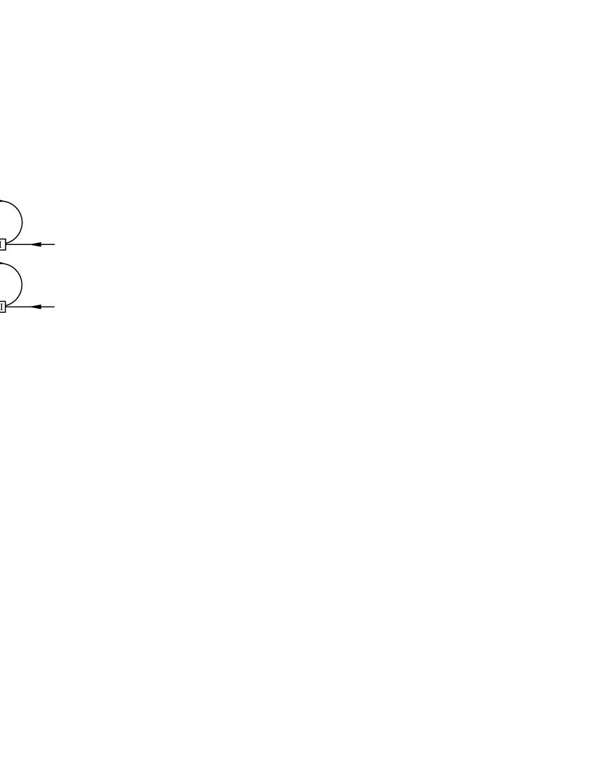
Figure 3: One-loop corrections to the lattice propagator (II). The numbers associated with the vertices refer to $H_{\text{int}}^{(\text{I})}$ and $H_{\text{int}}^{(\text{II})}$ of Eq. (23).

IV.1 One-loop correction to the magnon self-energy

The graphs occurring at the one-loop approximation are given in FIG 3. The explicit form of the correction arising from the first vertex is easily found using Feynman rules defined above:

$$\Sigma_{\text{I}}^{(1)}(\bm{k},\omega_{n}) = \begin{array}[]{l}\vspace{0.8cm}\includegraphics[scale={0.7}]{Fig8.eps}\end{array}.$$ (38)

It is understood that external legs, black and colored, are to be amputated. Further,

$$\Sigma_{\text{II}}^{(1)}(\bm{k},\omega_{n}) = \begin{array}[]{l}\vspace{0.8cm}\includegraphics[scale={0.7}]{Fig9_a.eps}\end{array}$$ (40)

$$+ \begin{array}[]{l}\vspace{0.8cm}\includegraphics[scale={0.7}]{Fig9_b.eps}\end{array}.$$ (42)

Since the first two diagrams of (42) vanish, by performing summation over the Matsubara frequencies, we obtain

$$\Sigma^{(1)}(\bm{k}) = \Sigma_{\text{I}}^{(1)}(\bm{k})+\Sigma_{\text{II}}^{(1)}(\bm{k})$$

$$= \frac{\widehat{\bm{k}}^{\;2}}{2m_{0}}\;\frac{1}{S}\frac{|\bm{\lambda}|^{2}}{2D}v_{0}\int_{\bm{q}}\langle n_{\bm{q}}\rangle_{0}\;\widehat{\bm{q}}^{\;2}$$

where we have exploited cubic symmetry of the lattice, and $\langle n_{\bm{q}}\rangle_{0}$ represents the Bose distribution for free magnons. According to (IV.1), magnons acquire mass

$$[m_{\text{r}}^{(1)}]^{-1} = m_{0}^{-1}\left[1-\frac{1}{S}\frac{|\bm{\lambda}|^{2}}{2D}v_{0}\int_{\bm{q}}\langle n_{\bm{q}}\rangle_{0}\widehat{\bm{q}}^{\;2}\right]$$ (44)

$$\equiv m_{0}^{-1}[1-A(T)]$$

This result can be made self-consistent bu further summation, i. e. by replacing the propagators with full Green’s functions in (38) and (42)

$$[m_{\text{R}}^{(1)}]^{-1}=m_{0}^{-1}\left[1-\frac{1}{S}\frac{|\bm{\lambda}|^{2}}{2D}v_{0}\int_{\bm{q}}\langle n_{\bm{q}}\rangle\widehat{\bm{q}}^{\;2}\right],$$ (45)

with $\langle n_{\bm{q}}\rangle$ denoting the Bose distribution for magnons with energies $\widehat{\bm{q}}^{2}/(2m_{\text{R}}^{(1)})$. If constant $F^{2}$ is chosen so that $H_{0}$ of (22) fully coincides with (II), i.e.

$$F^{2}=\frac{\Sigma}{2m_{0}}=\frac{JS^{2}Z_{1}|\bm{\lambda}|^{2}}{2Dv_{0}}$$ (46)

then $\widehat{\bm{k}}^{2}/(2m_{\text{R}}^{(1)})$ is precisely renormalized spin-wave energy, obtained for the first time in MBloch by minimization of the free energy of a ferromagnet, where the spin Hamiltonian (1) is written in terms of Dyson-Maleev (DM) bosons with only diagonal part of the interaction being retained. It was also obtained by the bubble diagram summation Loly , again using DM representation. However, only the derivation of (45) using effective Lagrangian clearly shows that the effects of two distinct types of magnon-magnon interactions are accounted for in (45).

IV.2 One-loop approximations for the spontaneous magnetization

The one-loop corrections to the LSWT result for spontaneous magnetization are found by substituting magnon propagator with Green’s function calculated to the one loop in (15). This is easily obtained by keeping the external legs in (38) and (42). The result is

$$\langle S^{z}\rangle = S-v_{0}\int_{\bm{p}}\langle n_{\bm{p}}\rangle_{0}+\delta\langle S^{z}\rangle,$$

$$\delta\langle S^{z}\rangle = -v_{0}\int_{\bm{p}}\frac{\Sigma^{(1)}(\bm{p})\langle n_{\bm{p}}\rangle_{0}[\langle n_{\bm{p}}\rangle_{0}+1]}{T}.$$ (47)

There is an obvious virtue in writing the spontaneous magnetization as in Eq. (47). The term $S-v_{0}\int_{\bm{q}}\langle n_{\bm{q}}\rangle_{0}$ describes the reduction of spontaneous magnetization due to free magnons. Its low-temperature expansion for 3D HFM contains well known contributions proportional to $T^{3/2}$(Bloch’s law), $T^{5/2}$, $T^{7/2}$ and so on. On the other hand, the corrections arising from the magnon-magnon interactions are entirely collected in the integral proportional to $1/T$. More generally, the low-temperature series for spontaneous magnetization of a $D-$dimensional simple cubic HFM in the one-loop approximation consists of two parts

$$\langle S^{z}\rangle = S+\delta\langle S^{z}\rangle_{\text{free}}+\delta\langle S^{z}\rangle_{\text{int}},$$ (48)

where

$$\delta\langle S^{z}\rangle_{\text{free}} = \alpha_{0}T^{D/2}+\alpha_{1}T^{(D+2)/2}+\alpha_{2}T^{(D+4)/2}$$ (49)

$$+ \alpha_{3}T^{(D+6)/2}+{\mathcal{O}}\left(T^{(D+8)/2}\right)$$

and the free-magnon coefficients $\alpha_{i}$ are given by

$$\alpha_{0} = -\left(\frac{1}{2\sqrt{\pi}}\right)^{D}\frac{\sqrt{\pi}}{\Gamma(D/2)}\zeta\left(\frac{D}{2}\right)\left[\frac{\Sigma a^{2}}{F^{2}}\right]^{D/2},$$

$$\alpha_{1} = -\left(\frac{1}{2\sqrt{\pi}}\right)^{D}\frac{D}{16}\;\zeta\left(\frac{D+2}{2}\right)\left[\frac{\Sigma a^{2}}{F^{2}}\right]^{\frac{D+2}{2}},$$

$$\alpha_{2} = -\left(\frac{1}{2\sqrt{\pi}}\right)^{D}\frac{D\left[D+8\right]}{512}\zeta\left(\frac{D+4}{2}\right)\left[\frac{\Sigma a^{2}}{F^{2}}\right]^{\frac{D+4}{2}},$$

$$\alpha_{3} = -\left(\frac{1}{2\sqrt{\pi}}\right)^{D}\frac{D}{3072}\;\zeta\left(\frac{D+6}{2}\right)\left[\frac{\Sigma a^{2}}{F^{2}}\right]^{\frac{D+6}{2}}$$ (50)

$$\times \left[25+3D+\frac{D^{2}}{8}\right].$$

The temperature expansion of one-loop correction to LSWT results is

$$\delta\langle S^{z}\rangle_{\text{int}} = \beta_{1}T^{D+1}+\beta_{2}T^{D+2}+{\mathcal{O}}\left(T^{D+3}\right),$$ (51)

with

$$\beta_{1} = -\frac{1}{S}\left(\frac{1}{2\pi}\right)^{2D}\frac{D\pi^{D}}{8}\left[\frac{\Sigma a^{2}}{F^{2}}\right]^{D+1}$$

$$\times \zeta\left(\frac{D}{2}\right)\zeta\left(\frac{D+2}{2}\right),$$

$$\beta_{2} = -\frac{1}{S}\left(\frac{1}{2\pi}\right)^{2D}\frac{D[D+2]\pi^{D}}{128}\left[\frac{\Sigma a^{2}}{F^{2}}\right]^{D+2}$$ (52)

$$\times \left\{\left[\zeta\left(\frac{D+2}{2}\right)\right]^{2}+\zeta\left(\frac{D}{2}\right)\zeta\left(\frac{D+4}{2}\right)\right\}.$$

In the formulae above, $\zeta(x)$ denotes the Riemann zeta function and $D\geq 3$ is understood.

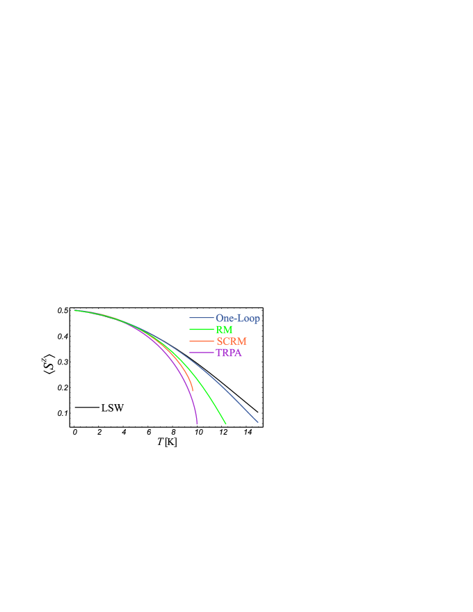
Figure 4: (Color online) Spontaneous magnetization of $S=1/2$ and $J=10$K 3D HFM calculated using LSWT (Eq. (15)), Tyablikov RPA, one-loop approximation (47), renormalized magnons (RM) of (44) and self-consistent renormalized magnons (SCRM) given in (45).

For $D=3$, the lowest order correction from magnon-magnon interaction comes to be $\propto T^{4}$, in agreement with Dyson Dyson2 . We note that the correct form of leading order contribution is found easily, evaluating only a single type of diagram indicated at FIG 3. This should be compared with continuum field-theoretical calculations Hofmann2 ; Hofmann3 , where number of diagrams to be evaluated becomes greater with increasing dimensionality of the lattice (see also the Section VI). Also, the lattice regularized theory allows for a comparison with LSWT and other methods, such as Tyablikov RPA, even at not too low temperatures.

The plot of spontaneous magnetization of spin $S=1/2$ and exchange integral $J=10$K calculated by LSWT (Eq. (15)), Tyablikov RPA, the one-loop approximation of Eq. (47) and dressed magnons of (44) and (45) is presented at FIG. 4. We have set $F^{2}=JS\Sigma a^{2}$ in (47) to work with a common energy scale. The TRPA result for $T_{\text{C}}$ is $\approx 10.065$ K (For precise calculation of the critical temperature in TRPA, see SSCTNRPA ; JPA and references therein).

IV.3 Two-loop corrections to the self-energy

The self-energy graphs with two loops, involving vertices $\begin{array}[]{r}{\includegraphics[scale={1.0}]{Fig3_a.eps}}\end{array}$ and $\begin{array}[]{r}{\includegraphics[scale={1.0}]{Fig3_b.eps}}\end{array}$ can be classified in two groups. Graphs presented at FIG 5 contribute purely to the magnon mass, i.e. they have no imaginary parts.

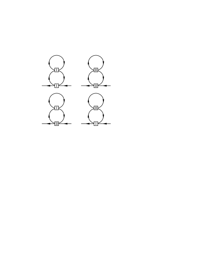
Figure 5: Two-loop graphs for magnon self-energy that contribute solely to the magnon mass.

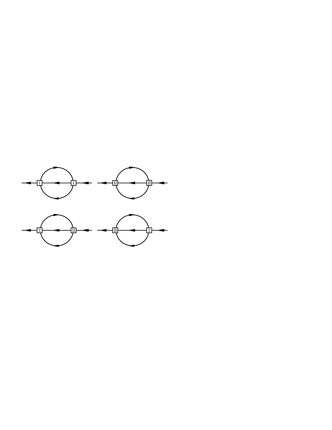
Figure 6: Two-loop diagrams for magnon self-energy that cause finite magnon lifetime.

The diagrams from FIG 6, however, produce the finite magnon lifetime. (The influence of finite magnon lifetime shall not be discussed further in the present paper. For details and references, see KaganovChubukov ; Harris ; Zitomirski .) All these diagrams can be evaluated using formalism of colored propagators, as explained in III.3. An example for decomposition of compact two-loop diagram of FIG 6 into its momentum-space contractions is given at FIG 2. Note that there are only two distinct Matsubara summations at the two-loop. The first one is common to all graphs from FIG 5 and the second one appears in all graphs form FIG 6, since the lattice Laplacian leaves $n$-index untouched.

The diagrams from FIG 5 then evaluate to

$$\Sigma_{\text{FIG 5}}(\bm{k}) = \frac{1}{S}\frac{\widehat{\bm{k}}^{2}}{2m_{0}}\frac{2D}{|\bm{\lambda}|^{2}}\;\frac{\alpha(T)}{2m_{0}T}\left[\frac{|\bm{\lambda}|^{2}}{2D}\right]^{2}v_{0}\int_{\bm{p}}\frac{\langle n_{\bm{p}}\rangle_{0}[\langle n_{\bm{p}}\rangle_{0}+1]}{T}\left[\widehat{\bm{p}}^{\;2}\right]^{2}\equiv\frac{\widehat{\bm{k}}^{2}}{2m_{0}}A(T)B(T)$$ (53)

The contribution from diagrams presented at FIG 6 consist of two parts, both of which change the geometry of magnon dispersion: The first part is proportional to $\widehat{\bm{k}}^{2}$

$$\Sigma_{\text{FIG 6}}^{(a)}(k) = \frac{1}{2S^{2}}\frac{\widehat{\bm{k}}^{2}}{[2m_{0}]^{2}}\left[\frac{|\bm{\lambda}|^{2}}{2D}\right]^{2}v_{0}^{2}\int_{\bm{p},\bm{q}}F^{\bm{k}}_{\bm{p},\bm{q}}(\text{i}\omega_{n})\widehat{\bm{q}}^{\;2}\widehat{\bm{p}}^{\;2}\left[\widehat{\bm{q}}^{\;2}-\widehat{\bm{p}-\bm{q}}^{\;2}\right]$$ (54)

and the other one to $\widehat{\bm{k}}^{4}$

$$\Sigma_{\text{FIG 6}}^{(b)}(k) = \frac{1}{2S^{2}}\left[\frac{\widehat{\bm{k}}^{2}}{2m_{0}}\right]^{2}\left[\frac{|\bm{\lambda}|^{2}}{2D}\right]^{2}v_{0}^{2}\int_{\bm{p},\bm{q}}F^{\bm{k}}_{\bm{p},\bm{q}}(\text{i}\omega_{n})\widehat{\bm{q}}^{\;2}\left[\widehat{\bm{q}}^{\;2}-\widehat{\bm{p}-\bm{q}}^{\;2}\right].$$ (55)

We have introduced here a shorthand notation for the vertex function, obtained by double Matsubara-index summation

$$F^{\bm{k}}_{\bm{p},\bm{q}}(\text{i}\omega_{n})=\frac{\langle n_{\bm{p}}\rangle_{0}[1+\langle n_{\bm{q}}\rangle_{0}+\langle n_{\bm{k}+\bm{p}-\bm{q}}\rangle_{0}]-\langle n_{\bm{q}}\rangle_{0}\langle n_{\bm{k}+\bm{p}-\bm{q}}\rangle_{0}}{\omega_{0}(\bm{k}+\bm{p}-\bm{q})-\omega_{0}(\bm{p})+\omega_{0}(\bm{q})-\text{i}\omega_{n}}.$$

From (IV.1), (53), (54) and (55), we find the magnon energies at two loop

$$\omega_{\text{2loop}}(\bm{k}) = \omega_{0}(\bm{k})-\delta\omega_{\text{2loop}}(\bm{k}),\hskip 28.45274pt\delta\omega_{\text{2loop}}(\bm{k})=\lim_{\delta\rightarrow 0}\text{Re}\Sigma(\bm{k},\omega_{0}(\bm{k})+\text{i}\delta),$$ (56)

$$\Sigma(\bm{k},\omega_{0}(\bm{k})+\text{i}\delta) = \Sigma^{(1)}(\bm{k})+\Sigma_{\text{FIG 5}}(\bm{k})+\Sigma_{\text{FIG 6}}^{(a)}\left(\bm{k},\omega_{0}(\bm{k})+\text{i}\delta\right)+\Sigma_{\text{FIG 6}}^{(b)}\left(\bm{k},\omega_{0}(\bm{k})+\text{i}\delta\right)$$ (57)

$$= \frac{\widehat{\bm{k}}^{2}}{2m_{0}}\left[A(T)+A(T)B(T)\right]$$

$$+ \frac{\widehat{\bm{k}}^{2}}{2m_{0}}\frac{1}{2S^{2}}\left[\frac{|\bm{\lambda}|^{2}}{2D}\right]^{2}\frac{v_{0}^{2}}{2m_{0}}\int_{\bm{p},\bm{q}}F^{\bm{k}}_{\bm{p},\bm{q}}\left(\omega_{0}(\bm{k})+\text{i}\delta\right)\widehat{\bm{q}}^{\;2}\left(\widehat{\bm{p}}^{\;2}+\widehat{\bm{k}}^{\;2}\right)\left(\widehat{\bm{q}}^{\;2}-\widehat{\bm{p}-\bm{q}}^{\;2}\right).$$

It is seen from (57) that magnons remain gapless at two loop ($\omega_{\text{2loop}}(\bm{k})\rightarrow 0$ as $|\bm{k}|\rightarrow 0$) just as do pions in Lorentz-invariant models Smilga ; Lewis ; StrangeMass .

On FIG 7 we plot the free-magnon dispersion $\omega_{0}(k_{x},k_{y},0)$ [Equation (11)] for $J=10$K, $S=1/2$ and $T=1$K, along with $\delta\omega_{\text{2loop}}(k_{x},k_{y},0)$. The numerical values of magnon mass renormalizating factors are $A=2.849\times 10^{-4}$ and $B=7.298\times 10^{-4}$.

IV.4 TRPA as an effective field theory

Now that the picture of HFM as a interacting magnon field is complete, we can make some observation on TRPA result for spontaneous magnetization and free energy. They may not be apparent, or even accessible within conventional TGF methodology or any other approach that relies on boson/fermion representation of spin operators. Present derivation of TRPA dispersion relation for magnons, and latter discussion on spurious $T^{3}$ term, clearly isolates the influence of retained magnon-magnon interactions from the neglection of short-ranger fluctuations in mean number of magnons per lattice site.

Consider a system of magnons for which the free Lagrangian is (19) and interaction is described by $\widetilde{{\mathcal{L}}}_{\text{int}}$ obtained from (20) by neglecting the second term proportional to $\bm{\pi}\cdot\Delta\bm{\pi}$ and keeping only $\sqrt{1-\bm{\pi}^{2}}$ in the square bracket. Corresponding Hamiltonian that includes up to four magnon operators, $\widetilde{H}=H_{0}+\widetilde{H}_{\text{int}}$, is easily constructed. Since $\widetilde{H}_{\text{int}}=-H_{\text{int}}^{(\text{II})}$, the one-loop self energy is found from (42)

$$\widetilde{\Sigma}(\bm{k})=\frac{1}{S}\frac{v_{0}}{2m_{0}}\int_{\bm{p}}\langle n_{\bm{p}}\rangle_{0}\;\widehat{\bm{p}-\bm{k}}^{2}.$$ (58)

We shall now assume that the mean number of excited magnons is the same at each lattice site. This simplification mimics TRPA replacement of the operator $S_{\bm{n}}^{z}$ with the site-independent average $\langle S^{z}\rangle$. Then

$$v_{0}\int_{\bm{p}}\langle n_{\bm{p}}\rangle_{0}\gamma(\bm{p})=v_{0}\int_{\bm{p}}\langle n_{\bm{p}}\rangle_{0}$$ (59)

equals the mean number of magnons on each lattice site, $\langle n_{\bm{x}}\rangle$. The magnon energies may now be written as

$$\widetilde{\omega}(\bm{k})=\omega_{0}(\bm{k})-\widetilde{\Sigma}(\bm{k})=\frac{\widehat{\bm{k}}^{2}}{2m_{0}}\frac{S-\langle n_{\bm{x}}\rangle}{S},$$ (60)

which we may, for low temperatures, identify with TRPA energies (16). In other words, the effective Hamiltonian of Tyablikov RPA, written in terms of lattice magnon fields is

$$\widetilde{H}\equiv H_{\text{eff}}^{\text{RPA}} = H_{0}+\frac{F^{2}}{8}v_{0}\sum_{\bm{x}}\bm{\pi}^{2}(\bm{x})\nabla^{2}\bm{\pi}^{2}(\bm{x})$$ (61)

with $H_{0}$ defined in (22). Reversing the arguments that lead to the $H_{\text{eff}}^{\text{RPA}}$, and also to the correct interacting Hamiltonian of lattice magnons (23), we see that TRPA results are generated starting from the leading order effective Lagrangian

$${\mathcal{L}}_{\text{eff}}^{\text{RPA}} = \frac{\Sigma}{2}\left(\partial_{t}U^{1}U^{2}-\partial_{t}U^{2}U^{1}\right)-\frac{F^{2}}{2}\partial_{\alpha}U^{i}\partial_{\alpha}U^{i}$$ (62)

$$- \frac{F^{2}}{4}\bm{\pi}^{2}(\bm{x})\Delta\bm{\pi}^{2}(\bm{x}).$$

This Lagrangian manifestly violates spin-rotational invariance of the original Heisenberg Hamiltonian (1).

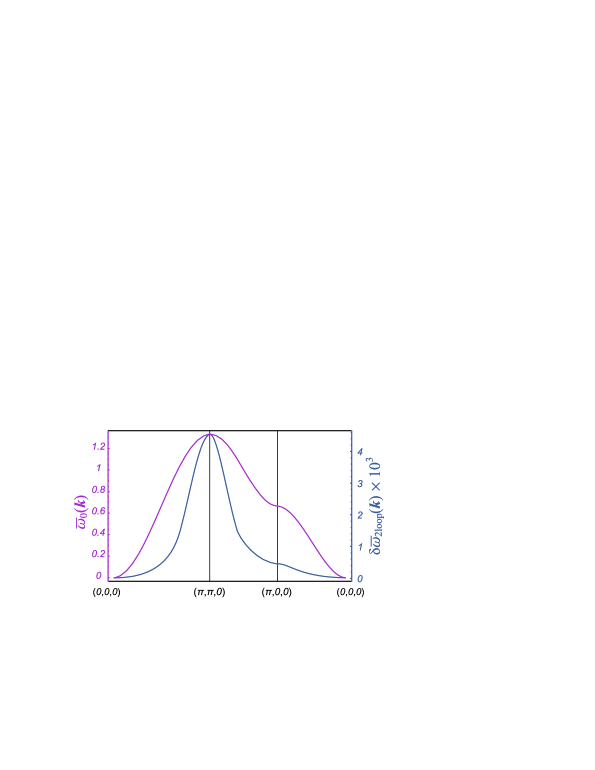
Figure 7: (Color online) Reduced free magnon energies $\bar{\omega}_{0}(\bm{k})=\omega_{0}(\bm{k})[m_{0}|\bm{\lambda}|^{2}/D]$ (left axis, purple curve) and 2-loop correction $\delta\bar{\omega}_{\text{2loop}}(\bm{k})=\delta\omega(\bm{k})_{\text{2loop}}[m_{0}|\bm{\lambda}|^{2}/D]$ (right axis, blue curve). $\omega_{0}(\bm{k})$ is defined in (11), and $\delta\omega_{\text{2loop}}(\bm{k})$ is given in (56) and (57). $S=1/2,D=3J=10\text{K}$ and $T=1$K for both curves

Various explanations for the spurious $T^{3}$ term in TRPA expansion of the ferromagnetic order parameter and the error caused by the Tyablikov decoupling at low temperatures have been offered by many authors. For example, in the Tyablikov’s monograph, it is attributed to the ”approximate character” (of the decoupling approximation) and the ”neglection of the fluctuation of order parameter” Tjablikov . In the context of the spin-diagram technique, authors of VLP1 ; VLP2 state that $T^{3}$ arises since ”in the decoupling methods terms after $r_{0}^{-3}$ are taken into the account incorrectly”. (Here $r_{0}^{-3}$ represents the formal expansion parameter in the spin-diagram technique, namely the reciprocal interaction volume.) In Fishman , the main feature of TRPA is recognized as being ”uncontrolled expansion to all orders in $1/Z_{1}$”. On the other hand, the authors of Stinchcombe conclude that erroneous $T^{3}$ term in TRPA ”comes from taking expectation values in the equation of motion too soon”. Finally, in Plakida , Tyablikov RPA is described as an approximation ”in which contributions of static fluctuations of spins are neglected”. However, it is also noted in this reference that $T^{3}$ term will appear in any approximation that incorrectly treats spectral density entering the correlation function $\langle S^{-}S^{+}\rangle_{\bm{k}}$. All arguments quoted above rely directly on the localized spin operators Tjablikov ; Plakida ; Fishman that define Heisenberg Hamiltonian (1) or on their boson/fermion representations VLP1 ; VLP2 ; Stinchcombe . The derivation of Tyablikov RPA in terms of lattice magnon fields, as given in the present paper, provides a simple and straightforward answer based on the internal symmetries of the Heisenberg model. It is seen from the equations (61)-(62) that Tyablikov RPA incorrectly describes O(3) HFM at low temperatures since it eventually results from the effective Lagrangian (62) that does not preserve spin-rotational symmetry of the Heisenberg ferromagnet (1). Explicitly, interactions of the form $\bm{\pi}^{2}\bm{\pi}\cdot\nabla^{2}\bm{\pi}$ arising from the WZW term $H_{\text{int}}^{(1)}$ are omitted in TRPA. It may also be said that due this reduction of magnon-magnon interactions in the effective Lagrangian, localized spins of HFM are inadequately described by the unit vector $\bm{U}(x)$.

We note that essential error in TRPA is made when magnon-magnon interactions arising from the WZW term are omitted. Neglection of the SRF of the order parameter, i.e. neglection of the fluctuations in the mean number of magnons at adjacent sites (the replacement of $v_{0}\int_{\bm{q}}\langle n_{\bm{q}}\rangle_{0}\gamma(\bm{q})$ with $v_{0}\int_{\bm{q}}\langle n_{\bm{q}}\rangle_{0}=\langle n_{\bm{x}}\rangle$) merely modifies coefficient of the $T^{3}$ term. To show this, we find the first order correction to the spontaneous magnetization based on Eq. (42)

$$\delta\langle S^{z}\rangle = -\frac{1}{S}\frac{F^{2}}{T\Sigma}v_{0}\int_{\bm{p}}J(\bm{p})\langle n_{\bm{p}}\rangle_{0}[\langle n_{\bm{p}}\rangle_{0}+1],$$

$$J(\bm{p}) = v_{0}\int_{\bm{q}}\langle n_{\bm{q}}\rangle_{0}(\widehat{\bm{p}-\bm{q}})^{2}.$$ (63)

The leading order term in temperature expansion of Eq. (63) for $D$ dimensional simple cubic lattice is

$$- \frac{1}{S}\frac{F^{2}D\pi^{D}}{2\Sigma}\left(\frac{a}{2\pi}\right)^{2D}\left[\frac{\Sigma}{F^{2}}\right]^{D+1}$$

$$\times \left\{\left[\zeta\left(\frac{D}{2}\right)\right]^{2}+\zeta\left(\frac{D}{2}+1\right)\zeta\left(\frac{D}{2}-1\right)\right\}T^{D}.$$

and for $D=3$, it corresponds to spurious $T^{3}$ term. If an additional assumption on the absence of SRF is included, the term $\propto\zeta\left(D/2+1\right)\zeta\left(D/2-1\right)$ is missing from (IV.4). The Tyablikov’s $T^{3}$ term Tjablikov ; TerHaar ,

$$- \frac{3}{2S}\left(\frac{1}{4\pi JS}\right)^{3}\left[\zeta\left(\frac{3}{2}\right)\right]^{2}T^{3}$$ (65)

is found by setting $F^{2}=JS\Sigma a^{2}$ (See (46)). An alternative formulation of O(2) model (61) is given in the Appendix B.

V Free energy at three-loop

For the subsequent analysis of the low temperature thermodynamics, we shall include weak external magnetic field directed along the 3-axis. It opens the gap in magnon spectrum

$$\omega(\bm{p})\longrightarrow\omega(\bm{p},H)=\omega(\bm{p})+\mu H,$$ (66)

and it is included in the effective Lagangian by standard Zeeman term PRD .

$${\mathcal{L}}_{H}=\Sigma\mu HU^{3}.$$ (67)

Note that the interaction Hamiltonian does not contain terms proportional to the external field $H$. This is an exact result to all orders in $\bm{\pi}^{2}$, and it follows from the equation of motion.

V.1 Two-loop correction to the free energy

The first-order correction to the free energy (see e.g. Kapusta ) of lattice magnons, involving the two-loop graphs, is given by

$$\delta F_{\text{2loop}}=-T\begin{array}[]{l}\includegraphics[scale={0.8}]{Fig14_a.eps}\end{array}-T\begin{array}[]{l}\includegraphics[scale={0.8}]{Fig15_a.eps}\end{array},$$ (70)

with the notation introduced in previous sections.

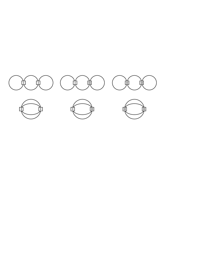
Figure 8: Six distinct three-loop diagrams contributing to the free energy.

According to the Feynman rules defined in III.3, these diagrams decompose to

$$\begin{array}[]{l}\includegraphics[scale={0.8}]{Fig14_a.eps}\end{array}=\begin{array}[]{l}\includegraphics[scale={0.8}]{Fig14_b.eps}\end{array}+\begin{array}[]{l}\includegraphics[scale={0.8}]{Fig14_c.eps}\end{array},$$ (74)

and

$$\begin{array}[]{l}\includegraphics[scale={0.8}]{Fig15_a.eps}\end{array}=\begin{array}[]{l}\includegraphics[scale={0.8}]{Fig15_b.eps}\end{array}+\begin{array}[]{l}\includegraphics[scale={0.8}]{Fig15_c.eps}\end{array},$$ (78)

so that the first correction to the free energy per lattice site is given by

$$\delta f_{\text{2loop}}=\frac{\delta F_{\text{2loop}}}{N}=-\frac{1}{S}\frac{F^{2}}{\Sigma}\frac{|\bm{\lambda}|^{2}}{4D}\left[v_{0}\int_{\bm{p}}\langle n_{\bm{p}}\rangle_{0}\;\widehat{\bm{p}}^{\;2}\right]^{2},$$ (79)

The temperature expansion of (79) starts with $T^{D+2}$ term. Specifically, for $D-$dimensional cubic lattices, it is

$$\delta f_{\text{2loop}} = -\frac{1}{S}\frac{D\pi^{D}}{16a^{D}}\left(\frac{1}{2\pi}\right)^{2D}\left(\frac{\Sigma a^{2}}{F^{2}}\right)^{D+1}T^{D+2}$$ (80)

$$\times \left[\sum_{n=1}^{\infty}\frac{\text{e}^{-\mu Hn/T}}{n^{(D+2)/2}}\right]^{2}+{\mathcal{O}}(T^{D+3}).$$

If $D=3$, this gives leading-order part of Dyson’s $T^{5}$ term Dyson2 . It receives contribution from higher-loop diagrams in the lattice regularized theory (see the subsection V.3).

At this point we also justify one-loop calculation of spontaneous magnetization from previous section by showing that corrections to LSWT from (47) can be obtained from the first-order correction to the free energy of lattice magnons. The first correction to spontaneous magnetization (per lattice site) is $\delta\langle S^{z}\rangle=-\partial(\delta f_{\text{2loop}})/\partial(\mu H)|_{H=0}$. Differentiating (79) with respect to $\mu H$ and setting $H=0$ we readily recover equation (47).

V.2 Three-loop corrections to the free energy

Three-loop contribution to the magnon free energy is represented by diagrams from FIG 8. They can be classified into two categories, distinguished by $a$ and $b$ superscripts in the following equations.

Each of the three upper diagrams from FIG 8, to be classified as $a$-type, consists of a number of different colored contractions. For the graph containing vertices solely from $H_{\text{int}}^{(\text{I})}$, each of distinct colored contractions repeats four times, so that

$$\delta f_{\text{I,I}}^{(a)} = -\frac{1}{2S^{2}}\left[\frac{1}{2m_{0}}\right]^{2}v_{0}^{3}\int_{\bm{k},\bm{p},\bm{q}}\frac{\langle n_{\bm{q}}\rangle_{0}[\langle n_{\bm{q}}\rangle_{0}+1]}{T}$$ (81)

$$\times \langle n_{\bm{p}}\rangle_{0}\langle n_{\bm{k}}\rangle_{0}\left[\widehat{\bm{p}}^{2}\widehat{\bm{q}}^{2}+\widehat{\bm{k}}^{2}\widehat{\bm{q}}^{2}+\widehat{\bm{p}}^{2}\widehat{\bm{k}}^{2}+\widehat{\bm{q}}^{2}\widehat{\bm{q}}^{2}\right].$$

Further, for the graph with two vertices from $H_{\text{int}}^{(\text{II})}$, we find

$$\delta f_{\text{II,II}}^{(a)} = -\frac{1}{2S^{2}}\left[\frac{1}{2m_{0}}\right]^{2}v_{0}^{3}\int_{\bm{k},\bm{p},\bm{q}}\frac{\langle n_{\bm{q}}\rangle_{0}[\langle n_{\bm{q}}\rangle_{0}+1]}{T}$$ (82)

$$\times \langle n_{\bm{p}}\rangle_{0}\langle n_{\bm{k}}\rangle_{0}\left[\widehat{\bm{p}-\bm{q}}^{2}\widehat{\bm{k}-\bm{q}}^{2}\right].$$

This term consists of two different colored contractions, each appearing twice. The total contribution of the graphs that involve vertices of both $H_{\text{int}}^{(\text{I})}$ and $H_{\text{int}}^{(\text{II})}$ is

$$\delta f_{\text{I,II}}^{(a)} = \frac{1}{S^{2}}\left[\frac{1}{2m_{0}}\right]^{2}v_{0}^{3}\int_{\bm{k},\bm{p},\bm{q}}\frac{\langle n_{\bm{q}}\rangle_{0}[\langle n_{\bm{q}}\rangle_{0}+1]}{T}$$ (83)

$$\times \langle n_{\bm{p}}\rangle_{0}\langle n_{\bm{k}}\rangle_{0}\left[\widehat{\bm{p}}^{2}\;\widehat{\bm{k}-\bm{q}}^{2}+\widehat{\bm{q}}^{2}\;\widehat{\bm{k}-\bm{q}}^{2}\right].$$

In this case, one of the colored contractions appears eight times and the other two four times each.

Finally, by putting contributions (81)-(83) together, we find the first part of three-loop contribution to the magnon free-energy per lattice site

$$\delta f_{\text{3loop}}^{(a)} = -\frac{1}{2S^{2}}\left[\frac{1}{2m_{0}}\right]^{2}v_{0}\int_{\bm{q}}\frac{\langle n_{\bm{q}}\rangle_{0}[\langle n_{\bm{q}}\rangle_{0}+1]}{T}\left[v_{0}\int_{\bm{p}}\langle n_{\bm{p}}\rangle_{0}\left(\widehat{\bm{p}-\bm{q}}^{2}-\widehat{\bm{p}}^{2}-\widehat{\bm{q}}^{2}\right)\right]^{2}.$$ (84)

The calculation resumes in a similar manner for remaining diagrams of $b$-type, i.e. for lower three diagrams of FIG 8. They add up to

$$\delta f_{\text{3loop}}^{(b)} = -\frac{1}{8S^{2}}\left[\frac{1}{2m_{0}}\right]^{2}v_{0}^{3}\int_{\bm{k},\bm{p},\bm{q}}G^{\bm{q}}_{\bm{k}.\bm{p}}\left[(\widehat{\bm{k}+\bm{p}-\bm{q}})^{2}+\widehat{\bm{q}}^{2}-\widehat{\bm{p}-\bm{q}}^{2}-\widehat{\bm{k}-\bm{q}}^{2}\right]\left[\widehat{\bm{p}}^{2}+\widehat{\bm{k}}^{2}-\widehat{\bm{p}-\bm{q}}^{2}-\widehat{\bm{k}-\bm{q}}^{2}\right]$$ (85)

with three-index Matsubara sum

$$G^{\bm{q}}_{\bm{k},\bm{p}}=\frac{\langle n_{\bm{k}}\rangle_{0}\langle n_{\bm{p}}\rangle_{0}[1+\langle n_{\bm{q}}\rangle_{0}+\langle n_{\bm{k}+\bm{p}-\bm{q}}\rangle_{0}]-\langle n_{\bm{q}}\rangle_{0}\langle n_{\bm{k}+\bm{p}-\bm{q}}\rangle_{0}[\langle n_{\bm{k}}\rangle_{0}+\langle n_{\bm{p}}\rangle_{0}+1]}{\omega_{0}(\bm{k}+\bm{p}-\bm{q})+\omega_{0}(\bm{q})-\omega_{0}(\bm{p})-\omega_{0}(\bm{k})}.$$

Now we consider limit $a\rightarrow 0$ and examine three-loop integrals (84) and (85) in detail.

V.3 Analysis of the three-loop integrals

First, it is easily seen that $\delta f_{\text{3loop}}^{(a)}$ vanishes in continuum limit, thus contributing nothing when the lattice anisotropies are neglected. This was pointed out in Hofmann3 for $D=3$. Its lowest order contribution is proportional to $T^{[3D+6]/2}$. For $D$ dimensional simple cubic lattice, this term is

$$- \frac{v_{0}}{\Sigma^{2}}\left(\frac{\Sigma}{F^{2}}\right)^{(3D+4)/2}\left(\frac{a^{2}}{2D}\right)^{2}\frac{D^{3}[D+2]}{32}$$ (86)

$$\times \left(\frac{1}{2\sqrt{\pi}}\right)^{3D}\left[\zeta\left(\frac{D+2}{2}\right)\right]^{3}T^{[3D+6]/2}.$$

It turns out, however, that this is not the leading order correction to the Dyson’s $T^{D+2}$ term.

The leading order correction to $T^{D+2}$ term in the low-temperature expansion of free energy originates in $\delta f_{\text{3loop}}^{(b)}$ of (85), but the continuum limit of these diagrams should be handled with care. In the direct continuum limit ($a\rightarrow 0$), integral (85) consists of two parts. The first one, containing two Bose-distributions, is UV divergent for all values of $D\geq 3$. Instead of subtracting this infinite contribution, we may fully exploit the lattice regularization to remove the divergent term. If the wave vectors, whose energies does not appear in Bose factors of (85), are kept within Brilouin zone, we find that first part of $\delta f_{\text{3loop}}^{(b)}$ renormalizes (79), i.e. (80): $\delta f_{\text{2loop}}\rightarrow\delta f_{\text{2loop}}[1+Q(D)/S]$. For the $D$ dimensional simple cubic lattice, the renormalizing factor is

$$Q(D)=\frac{1}{D}\int_{\bm{x}}\frac{\cos^{2}x_{1}}{1-\gamma_{D}(\bm{x})}.$$ (87)

Here $\bm{x}$ denotes dimensionless wave vector within Brilouin zone, $-\pi\leq x_{\alpha}\leq\pi,\;\;\alpha=1,2,\cdots D$.

Now we calculate the finite part of $\delta f_{\text{3loop}}^{(b)}$ in the continuum limit, the correction to (80) of order $T^{(3D+2)/2}$ due to magnon-magnon interactions. Introducing dimensionless wavevectors $\bm{x}=\bm{k}/\sqrt{2m_{0}T},\bm{y}=\bm{p}/\sqrt{2m_{0}T}$, and $\bm{z}=\bm{q}/\sqrt{2m_{0}T}$, we obtain the leading order term in $\delta f_{\text{3loop}}^{(b)}$:

$$\delta f_{\text{3loop}}^{(b)}(T,h)\approx-\frac{v_{0}}{\Sigma^{2}}\left(\frac{\Sigma}{F^{2}}\right)^{3D/2}I(D,h)\;T^{(3D+2)/2}$$ (88)

where

$$I(D,h)=\int_{\bm{x},\bm{y},\bm{z}}\frac{\langle n_{\bm{x}}(h)\rangle\langle n_{\bm{y}}(h)\rangle\langle n_{\bm{z}}(h)\rangle(\bm{x}\cdot\bm{y})^{2}}{\bm{z}^{2}+\bm{x}\cdot\bm{y}-\bm{z}\cdot(\bm{x}+\bm{y})}$$ (89)

and

$$\langle n_{\bm{x}}(h)\rangle=\left[\exp(\bm{x}^{2}+h)-1\right]^{-1},\;\;\;h=\mu H/T.$$ (90)

In the absence of external field $H$, (88) reduces to

$$\delta f_{\text{3loop}}^{(b)}(T)\approx-\frac{v_{0}}{\Sigma^{2}}\left(\frac{\Sigma}{F^{2}}\right)^{3D/2}I(D)\;T^{(3D+2)/2}$$ (91)

with $I(D)\equiv I(D,h=0)$. The numerical values of integrals $I(D)$ are listed in the Table 1 for $D=3,4,5$ and 6. We note that the value of the coefficient in $T^{11/2}$ term agrees perfectly with the calculations of Hofmann3 based on the dimensional regularization. For more details concerning numerical evaluation of the integrals $I(D)$, we refer to the Appendix A.

The result (91) enable us to calculate corresponding correction to the spontaneous magnetization induced by magnon-magnon interaction. Since $\delta\langle S^{z}\rangle=-\partial(\delta f_{\text{3loop}})/\partial(\mu H)|_{H=0}$, we find

$$\delta\langle S^{z}\rangle_{\text{int}}^{\text{3loop}}(T)\approx-\frac{v_{0}}{\Sigma^{2}}\left(\frac{\Sigma}{F^{2}}\right)^{3D/2}J(D)\;T^{3D/2}$$ (92)

where

$$J(D)=$$

$$- \int_{\bm{x},\bm{y},\bm{z}}\frac{\langle n_{\bm{x}}\rangle\langle n_{\bm{y}}\rangle\langle n_{\bm{z}}\rangle[3+\langle n_{\bm{x}}\rangle+\langle n_{\bm{y}}\rangle+\langle n_{\bm{z}}\rangle](\bm{x}\cdot\bm{y})^{2}}{\bm{z}^{2}+\bm{x}\cdot\bm{y}-\bm{z}\cdot(\bm{x}+\bm{y})}$$

and $\langle n_{\bm{x}}\rangle=\langle n_{\bm{x}}(h=0)\rangle$. The values of integrals $J(D)$ are also listed in Table 1. Again, for $D=3$, we find excellent agreement with Hofmann3 .

Table 1: Numerical values of integrals $I(D)$ and $J(D)$

$D$	$I(D)$	$J(D)$
$3$	$5.3367\times 10^{-6}$	$-4.401\times 10^{-5}$
$4$	$1.2287\times 10^{-7}$	$-6.565\times 10^{-7}$
$5$	$2.08596\times 10^{-9}$	$-1.9410\times 10^{-9}$
$6$	$1.40407\times 10^{-10}$	$-4.9436\times 10^{-10}$

At this point we may compare results from three-loop calculations for the free energy with those of section IV. The two leading order terms in low temperature series for the spontaneous magnetization due to magnon-magnon interactions were shown there to carry $D+1$ and $D+2$ powers of temperature, respectively. Results of three-loop analysis for the free energy reveal term with $3D/2$ powers of temperature. For $D=3$, the $T^{3D/2}$ term indeed represents the first correction to Dyson’s $T^{D+1}$ result. However, already for $D=4$, contribution from $T^{D+2}$ and $T^{3D/2}$ terms are of the same order. For $D\geq 5$ leading order correction to Dyson-like $T^{D+1}$ term is proportional to $T^{D+2}$, and is given in (51) and (52). Further understanding of relationship between $T^{D+2}$ and $T^{3D/2}$ terms may be reached by directly examining diagrammatic series for low-temperature expansion of free energy (see VI.2).

VI Symmetry of the effective Lagrangian and Spurious terms in low-temperature expansions

To gain further insight into the thermodynamics of $D$ dimensional $\text{O}(3)$ Heisenberg ferromagnet$-$in particular to see how various terms in the low-temperature expansion of free energy are generated by magnon-magnon interactions $-$ we shall now obtain the most important results of Section V with the help of power counting scheme for magnon fields. The power counting schemes and structure of diagrams for low-temperature expansion of the free energy in cases $D=2$ and $D=3$ are given in Hofmann3 ; Hofmann4 . We shall now generalize these results for arbitrary $D\geq 3$. In this section, the focus will be on the free energy per unit volume ($f=F/V$), in contrast to the Section V, devoted to the calculation of the free energy per lattice site.

VI.1 Effective Lagrangian and power counting

Following e.g DombreRead , we start from the lattice Hamiltonian (22), and obtain continuous Hamiltonian density up to $|\bm{p}|^{6}$, organized in the powers of magnon momenta. We also include weak external magnetic field $\bm{H}=H\bm{e}_{z}$

$${\mathcal{H}}_{0} = \frac{F^{2}}{2}\partial_{\alpha}\bm{\pi}\cdot\partial_{\alpha}\bm{\pi}-\Sigma\mu H\left(1-\bm{\pi}^{2}/2\right),$$

$${\mathcal{H}}^{(2)} = \frac{F^{2}}{8}\left[\bm{\pi}^{2}\bm{\pi}\cdot\Delta\bm{\pi}-\bm{\pi}^{2}\Delta\bm{\pi}^{2}\right]\equiv{\mathcal{H}}^{(2)}_{\text{I}}+{\mathcal{H}}^{(2)}_{\text{II}},$$

$${\mathcal{H}}^{(4)} = -l_{1}\partial_{\alpha}^{2}\bm{\pi}\cdot\partial_{\alpha}^{2}\bm{\pi}$$

$$+ \frac{l_{1}}{4}\left[\partial_{\alpha}^{2}\left(\bm{\pi}^{2}\bm{\pi}\right)\cdot\partial_{\alpha}^{2}\bm{\pi}-\partial_{\alpha}^{2}\bm{\pi}^{2}\partial_{\alpha}^{2}\bm{\pi}^{2}\right],$$

$${\mathcal{H}}^{(6)} = c_{1}\partial_{\alpha}^{3}\bm{\pi}\cdot\partial_{\alpha}^{3}\bm{\pi}$$

$$+ \frac{c_{1}}{4}\left[-\partial_{\alpha}^{3}\left(\bm{\pi}^{2}\bm{\pi}\right)\cdot\partial_{\alpha}^{3}\bm{\pi}+\partial_{\alpha}^{3}\bm{\pi}^{2}\partial_{\alpha}^{3}\bm{\pi}^{2}\right].$$

${\mathcal{H}}_{0}$ describes free magnons with rotationally invariant classical dispersion

$$E(\bm{k})=\frac{F^{2}}{\Sigma}\bm{k}^{2}+\mu H,$$ (95)

and the rest of terms in (VI.1) are treated as a perturbation. While first terms in ${\mathcal{H}}^{(4)}$ and ${\mathcal{H}}^{(6)}$ modify dispersion due to the lattice anisotropies, the other contributions include magnon-magnon interactions. The formal values for coupling constants are $l_{1}=F^{2}a^{2}/24,\;c_{1}=F^{2}a^{4}/720$. This Hamiltonian is seen to arise from the Lagrangian

$${\mathcal{L}}={\mathcal{L}}^{(2)}+{\mathcal{L}}^{(4)}+{\mathcal{L}}^{(6)}$$ (96)

where ${\mathcal{L}}^{(2)}$ is given in (17)

$${\mathcal{L}}^{(2)} = \Sigma\frac{\partial_{t}U^{1}U^{2}-\partial_{t}U^{2}U^{1}}{1+U^{3}}-\frac{F^{2}}{2}\partial_{\alpha}\bm{U}\cdot\partial_{\alpha}\bm{U}$$ (97)

$$+ \Sigma\mu HU^{3},$$

and

$${\mathcal{L}}^{(4)}=l_{1}\;\partial_{\alpha}^{2}\bm{U}\cdot\partial_{\alpha}^{2}\bm{U},\hskip 14.22636pt{\mathcal{L}}^{(6)}=c_{1}\;\bm{U}\cdot\partial_{\alpha}^{3}\partial_{\alpha}^{3}\bm{U}.$$ (98)

We see that, unlike spin-rotation symmetry, space-rotation symmetry is lost starting from $\bm{p}^{4}$ terms. The crucial point in systematic EFT calculation of the free energy density comes from the observation that loop diagrams carry additional powers of momentum and thus yield terms with increasing powers of temperature. For the model of current interest, each loop is suppressed by $D$ powers of momentum, as can bee seen from (II) [See also Hofmann2 ; Hofmann3 ; Hofmann4 ]. This, along with the fact that $\bm{p}^{2}$ counts as $T$, allows for systematic organization of diagrams contributing free energy density Gerber .

Before discussing the low-temperature expansion, we note that the single vertex three-lop diagrams

$$\begin{array}[]{l}\includegraphics[scale={0.8}]{Fig17.eps},\end{array}$$ (100)

with rectangle denoting vertices from ${\mathcal{H}}^{(2)},{\mathcal{H}}^{(4)}$ or ${\mathcal{H}}^{(6)}$ (i.e. $n=1,2,3$), are completely absent. This is true for all models containing only terms quadratic in $\bm{U}$ and consistent with symmetries of the Heisenberg model. To see how this happens, observe that WZW term always produce the six-magnon vertex with opposite sign than the one arising from terms with spatial derivatives only, as can be shown by employing the equation of motion. Thus, for model (96), cancellation of six-magnon vertices is exact to all orders in $|\bm{p}|$.

VI.2 Magnon magnon interactions and low-temperature series for the free energy density

Basically, two types of diagrams contribute to free energy. In the first of them, only vertices with two magnon fields appear. Their general form is

$$\begin{array}[]{l}\includegraphics[scale={0.8}]{Fig18.eps}\end{array}$$ (102)

where vertex with $2n_{i}$ powers of momentum appears $k_{i}$ times $(i=1,2,\cdots R)$. As loops are suppressed by $|\bm{p}|^{D}$ for Lagrangian (96), it is easy to see that diagrams of equation (102) contribute to low-temperature expansion of free energy with terms whose power of $T$ is $D/2+1+\sum_{i=1}^{R}k_{i}(n_{i}-1)$. All of them describe the influence of lattice anisotropies, i.e. they correspond to the $\alpha_{i}$ coefficients of the low-temperature expansion of spontaneous magnetization, given in (49). Since all two-magnon vertices carry an even power of momentum, contributions from lattice anisotropies produce the terms with powers of temperature equal to $D/2+1,D/2+2$ and so on.

The first diagram that describes magnon-magnon interaction involves a single four-magnon vertex of ${\mathcal{H}}^{(2)}$. By dimensional arguments, it contributes with a term proportional to $T^{D}$ in low-temperature expansion of free energy. However, this term vanishes due to the space-rotation symmetry Hofmann2 ; Hofmann3 . Moreover, we shall now show tat even general class of diagrams, containing four vertex of ${\mathcal{H}}^{(2)}$ and two-magnon vertices of ${\mathcal{H}}^{(2n)}$ always vanish, i.e. they do not contribute to the free energy of O(3) HFM. To this end, consider the diagram

$$\begin{array}[]{l}\includegraphics[scale={0.8}]{Fig19.eps}\end{array}$$ (104)

where we have, following standard conventions Gerber ; Hofmann2 ; Hofmann3 , denoted the vertex from ${\mathcal{H}}^{(2)}$ by a dot. The rectangles denote two-magnon vertices carrying $2n$ and $2m$ powers of $\bm{p}$, respectively. First, split the diagram (104) into two pieces, one including four-magnon vertex of ${\mathcal{H}}^{(2)}_{\text{I}}$ and the other one with vertex of ${\mathcal{H}}^{(2)}_{\text{II}}$ (i.e. $\begin{array}[]{l}\includegraphics[scale={1.0}]{Fig20_a.eps}\end{array}=\begin{array}[]{l}\includegraphics[scale={1.0}]{Fig20_b.eps}\end{array}+\begin{array}[]{l}\includegraphics[scale={1.0}]{Fig20_c.eps}\end{array}$). $\begin{array}[]{r}{\includegraphics[scale={1.0}]{Fig3_a.eps}}\end{array}$ and $\begin{array}[]{r}{\includegraphics[scale={1.0}]{Fig3_b.eps}}\end{array}$ bellow refer to ${\mathcal{H}}^{(2)}_{\text{I}}$ and ${\mathcal{H}}^{(2)}_{\text{II}}$ of (VI.1). Now

$$\begin{array}[]{l}\includegraphics[scale={0.8}]{Fig21_a.eps}\end{array} = \;\;\begin{array}[]{l}\includegraphics[scale={0.8}]{Fig21_b.eps}\end{array}+\;\;\begin{array}[]{l}\includegraphics[scale={0.8}]{Fig21_c.eps}\end{array}$$ (108)

$$+ \begin{array}[]{l}\includegraphics[scale={0.8}]{Fig21_d.eps}\end{array}+\begin{array}[]{l}\includegraphics[scale={0.8}]{Fig21_e.eps}\end{array},$$ (111)

$$\begin{array}[]{l}\includegraphics[scale={0.8}]{Fig22_a.eps}\end{array} = \;\;\begin{array}[]{l}\includegraphics[scale={0.8}]{Fig22_b.eps}\end{array}+\;\;\begin{array}[]{l}\includegraphics[scale={0.8}]{Fig22_c.eps}\end{array}$$ (115)

where first two diagrams in (111) and first one in (115) are to be multiplied by a factor of 2 and the rest of them by a factor of four. (The last two diagrams in (111), as well as the second one in (115) possess additional symmetry due to permutation of blue and green vertices.) There are four more colored contractions in equation (115) which we have not displayed, since they are of the form (34) and thus vanish. The diagrams from (111) and (115) are to be evaluated using diagrammatic rules from the Section III, modified to compensate the replacement of lattice magnon dispersion with (95). Finally, we see that diagram (104) is proportional to

$$\int_{\bm{p},\bm{q}}G(\bm{p},\bm{q},T)\;\bm{p}\cdot\bm{q}\left[2\text{p}^{2n}\text{p}^{2m}+\text{p}^{2n}\text{q}^{2m}\right]=0$$ (116)

with

$$G(\bm{p},\bm{q},T) = \frac{\langle n_{\bm{p}}\rangle[\langle n_{\bm{p}}\rangle+1]\langle n_{\bm{q}}\rangle[\langle n_{\bm{q}}\rangle+1]}{T^{2}},$$

$$\text{p}^{2n} = (-)^{n}\sum_{\alpha=1}^{D}p_{\alpha}^{2n}.$$

A special cases of vanishing diagram (104) are the ones with single two-magnon vertex or with four-magnon vertex only.

In a similar manner, one can also demonstrate the vanishing of three-loop diagram

$$\begin{array}[]{l}\includegraphics[scale={0.8}]{Fig23.eps}\end{array}$$ (118)

(see also Hofmann3 and discussion just before (86)).

Thus, a list of different diagrams arising from magnon-magnon interactions that actually contribute to the free energy of O(3) HFM is quite limited. The first term in the low-temperature expansion of the free energy density, carrying $D+2$ powers of temperature (the Dyson term), is generated by the two-loop diagram

$$\begin{array}[]{l}\includegraphics[scale={0.8}]{Fig24.eps}\end{array}.$$ (120)

Its value is

$$\delta f_{D+2} = -\frac{3l_{1}D\pi^{D}}{2\Sigma^{2}}\left(\frac{1}{2\pi}\right)^{2D}\left(\frac{\Sigma}{F^{2}}\right)^{D+2}T^{D+2}$$ (121)

$$\times \left[\sum_{n=1}^{\infty}\frac{\text{e}^{-\mu Hn/T}}{n^{(D+2)/2}}\right]^{2}.$$

Out of the two-loop graphs, now comes the $T^{D+3}$ term. It is given by

$$\begin{array}[]{l}\includegraphics[scale={0.8}]{Fig25_a.eps}\end{array}+\begin{array}[]{l}\includegraphics[scale={0.8}]{Fig25_b.eps}\end{array},$$ (124)

so that

$$\delta f_{D+3} = -\frac{3D\pi^{D}}{8\Sigma^{2}}\left(\frac{1}{2\pi}\right)^{2D}\left(\frac{\Sigma}{F^{2}}\right)^{D+3}T^{D+3}$$ (125)

$$\times \left[\frac{12l_{1}^{2}[D+4]}{F^{2}}-30c_{1}\right]$$

$$\times \sum_{n,m=1}^{\infty}\frac{\text{e}^{-\mu H[n+m]/T}}{n^{(D+2)/2}\;m^{(D+4)/2}}.$$

Next enter three-loop diagrams. The lowest non-zero diagram is

$$\begin{array}[]{l}\includegraphics[scale={0.8}]{Fig26.eps}\end{array}.$$ (127)

This diagram contains an infinite contribution (See the Section V). Its finite part is given by

$$\delta f_{3D/2+1} = -\frac{1}{\Sigma^{2}}\left(\frac{\Sigma}{F^{2}}\right)^{3D/2}I(D,h)\;T^{(3D+2)/2},$$ (128)

where numbers $I(D,h)$ are defined in (89). If the external magnetic field is switched off, equations (121), (125) and (128) give three lowest contributions to free energy density due to magnon-magnon interactions for $D=3,4$ and 5-dimensional ferromagnets. It was already mentioned, in the context of spontaneous magnetization, that $T^{3D/2+1}$ term of (128) represents the leading correction to the Dyson’s $T^{D+2}$ term only for $D=3$. This is understood quite naturally in the language of EFT: The $T^{3D/2+1}$-term comes from three-loop graph (127), and with increasing $D$ it is being pushed up in the temperature expansion compared to two-loop graphs (124). At $D=6$, one also needs to include four-magnon vertices of order $|\bm{p}|^{8}$ to calculate $T^{D+4}$ term from two-loop graphs, which is of the same order as $T^{3D/2+1}$ term of (127).

VI.3 Spurious terms

Now we examine in detail what is, in the section IV.4, shown to be the effective field theory for TRPA. The Hamiltonian density obtained from (61), up to the terms of order $|\bm{p}|^{6}$ reads

$${\mathcal{H}}^{(2)}_{\text{RPA}} = \frac{F^{2}}{8}\bm{\pi}^{2}\Delta\bm{\pi}^{2},$$

$${\mathcal{H}}^{(4)}_{\text{RPA}} = -l_{1}\partial_{\alpha}^{2}\bm{\pi}\cdot\partial_{\alpha}^{2}\bm{\pi}+\frac{l_{1}}{4}\partial_{\alpha}^{2}\bm{\pi}^{2}\partial_{\alpha}^{2}\bm{\pi}^{2},$$ (129)

$${\mathcal{H}}^{(6)}_{\text{RPA}} = c_{1}\partial_{\alpha}^{3}\bm{\pi}\cdot\partial_{\alpha}^{3}\bm{\pi}+\frac{c_{1}}{4}\partial_{\alpha}^{3}\bm{\pi}^{2}\partial_{\alpha}^{3}\bm{\pi}^{2}.$$

${\mathcal{H}}_{0}$ and the coefficients $l_{1}$ and $c_{1}$ are the same as ones in (VI.1). The corresponding Lagrangian up to $|\bm{p}|^{6}$ consists of three parts, ${\mathcal{L}}_{\text{RPA}}={\mathcal{L}}^{(2)}_{\text{RPA}}+{\mathcal{L}}^{(4)}_{\text{RPA}}+{\mathcal{L}}^{(6)}_{\text{RPA}}$, where each term contains contributions that explicitly break internal symmetry of the Heisenberg Hamiltonian (1)

$${\mathcal{L}}_{\text{RPA}}^{(2)} = \frac{\Sigma}{2}\left(\partial_{t}U^{1}U^{2}-\partial_{t}U^{2}U^{1}\right)-\frac{F^{2}}{2}\partial_{\alpha}\bm{U}\cdot\partial_{\alpha}\bm{U}$$ (130)

$$+ \Sigma\mu HU^{3}-\frac{F^{2}}{4}\bm{\pi}^{2}\Delta\bm{\pi}^{2},$$

$${\mathcal{L}}^{(4)}_{\text{RPA}} = l_{1}\partial_{\alpha}^{2}\bm{U}\cdot\partial_{\alpha}^{2}\bm{U}-\frac{l_{1}}{2}\bm{\pi}^{2}\partial_{\alpha}^{2}\partial_{\alpha}^{2}\bm{\pi}^{2},$$

$${\mathcal{L}}^{(6)}_{\text{RPA}} = l_{1}\partial_{\alpha}^{3}\bm{U}\cdot\partial_{\alpha}^{3}\bm{U}-\frac{l_{1}}{2}\bm{\pi}^{2}\partial_{\alpha}^{3}\partial_{\alpha}^{3}\bm{\pi}^{2}.$$

It is easily seen from (129) that TRPA contains the same one-loop diagrams (102) as correct effective theory for HFM defined by (VI.1). The most important difference in low temperature expansion concerns the two-loop diagram of four-magnon vertex ${\mathcal{H}}^{(2)}_{\text{RPA}}$. It is now given by

$$\begin{array}[]{l}\includegraphics[scale={0.8}]{Fig27_a.eps}\end{array} = \begin{array}[]{l}\includegraphics[scale={0.8}]{Fig27_b.eps}\end{array}+\begin{array}[]{l}\includegraphics[scale={0.8}]{Fig27_c.eps}\end{array}$$ (134)

so that

$$\delta f^{\text{RPA}}_{D+1} = -\frac{D\pi^{D}}{2\Sigma}\left(\frac{1}{2\pi}\right)^{2D}\left(\frac{\Sigma}{F^{2}}\right)^{2D}T^{D+1}$$ (135)

$$\times \sum_{n,m=1}^{\infty}\frac{\text{e}^{-\mu H[n+m]/T}}{n^{(D+2)/2}\;m^{D/2}}.$$

The dot in (134) represents four-magnon vertex of ${\mathcal{H}}^{(2)}_{\text{RPA}}$ from (129). Clearly, (135) is responsible for the spurious $T^{D+1}$ term (See the equations (IV.4) and (65)). In this manner, we have reached the same conclusion as in lattice regularized theory: the main reason for spurious $T^{D+1}$ term in low-temperature series for free energy is the explicit violation of internal symmetry of HFM by discarding magnon-magnon interactions from the WZW term. The effective action for TRPA Lagrangian is no longer O(3) invariant. Even though it was shown that space-rotation symmetry of leading order Lagrangian guaranties absence of $T^{D+1}$ term (See Hofmann2 ; Hofmann3 for $D=3$), we see that it only does so if the full spin-rotational symmetry of effective action is preserved (order by order, in the perturbative expansion).

The importance of WZW term in effective Lagrangian for ferromagnet was stressed in PRD ; WenZee where it was shown that it is crucial for obtaining correct qualitative magnon spectrum in linear approximation. The present paper puts conclusions of PRD ; WenZee a step forward in the sense that it is demonstrated how the thermodynamical properties of a ferromagnet depend on the magnon-magnon interactions generated by WZW term.

VII Sumarry

The method of effective Lagrangians is a powerful tool for analyzing the low-energy (low temperature) domain of models with strongly interacting constituents, provided spontaneous symmetry breaking occurs. Employed first for the description of low-energy sector of QCD, it soon found its way to the strongly correlated systems of condensed matter. A notable example for the latter class of systems is the isotropic Heisenberg ferromagnet, exhibiting $\text{O}(3)\longrightarrow\text{O}(2)$ spontaneous breakdown of internal spin-rotation symmetry. Due to a symmetry breakdown, massless particles (Goldstone bosons) appear in the spectrum. In the case of Heisenberg magnets, Goldstone bosons are called magnons and for O(3) HFM, there are two broken generators and a single magnon. The EFT line of reasoning then constitutes in writting the most general Lagrangian (i.e. action) consistent with internal symmetries of the Heisenberg Hamiltonian, organized in the powers of momenta of Goldstone fields. By employing appropriate Feynman rules for time-ordered Green’s functions of the effective Lagrangian, one can calculate free energy and other physical quantities of interest.

EFT is usually formulated in the functional integral framework using dimensional regularization. Lattice regularization, however, enables the effective Hamiltonian to inherit the full discrete symmetry of the original Heisenberg ferromagnet which modifies the free magnon dispersion from $\bm{k}^{2}/(2m_{0})$ to $\widehat{\bm{k}}^{2}/(2m_{0})$. In the spirit of chiral perturbation theory, where original quark and gluons of QCD are replaced with Goldstone bosons of spontaneously broken chiral symmetry, no reference is made to the original degrees of freedom, i. e. to the localized spins. The theory includes bosonic (magnon) fields from the beginning. Because of that, calculations in lattice EFT are free of certain types of approximations unavoidable in approaches relaying on equations of motion for spin operators or on their bosonic/fermionic representations. A vital part of our analysis is careful inclusion of the magnon-magnon interactions arising from the WZW term in the effective Lagrangian.

Calculations in EFT reduce to evaluation of various Feynman diagrams involving propagators of Goldstone fields. As Goldstone fields are derivatively coupled, the lattice regularization necessary induces diagrams containing at least one lattice Laplacian acting on propagators. The number of lattice Laplacians increases with the order of diagram, i.e. with number of loops. The structure of diagrams becomes even more involved if interaction part of Hamiltonian consists of several terms different in derivative structure since more than one lattice Laplacian may act on given propagator, as in the present paper. To get around these complications as much as possible, we have devised a variant of Feynman diagrams suitable for scalar fields with derivative couplings. They are applicable for lattice as well for continuum field theories. Corresponding Feynman rules are based on colored lines and vertices and are exposed in Section III.3. All calculations in the present paper rely on this version of Feynman diagrams.

Once the effective Hamiltonian of lattice magnon fields is found, it can be used to study magnon-magnon interactions and their influence on magnon self energy, spontaneous magnetization and free energy of $D\geq 3$ HMF. We have shown in Section IV that the Dyson’s correction to the spontaneous magnetization can be obtained from one-loop correction to the magnon propagator, bypassing discussion on the free energy. The approach simplifies calculations and opens direct link to the standard theories of spin waves in the Heisenberg ferromagnet. In particular, using EFT, we have established connection between theories on nonlinear spin waves, Tyablikov GF method and importance of magnon-magnon interactions originating in the WZW term. It is also shown in Section IV that, similarly to pions in Lorentz-invariant models, ferromagnetic magnons remain ”massless” at two-loop.

Further analysis of three-loop corrections to the free energy of HFM, presented in Sections V and VI, reveals how magnon-magnon interactions manifest themselves in the low-temperature series for free energy. The two-loop correction yields terms proportional to $T^{D+2}$, $T^{D+3}$ and so on, while the three-loop corrections start with term proportional to $3D/2+1$ powers of temperature. Discussion from Section VI shows how interplay between the number of loops and the spatial dimensionality of the lattice dictates structure of this low-temperature series. We also present numerical values for coefficients of $T^{3D/2+1}$ term in case of 3,4,5 and 6-dimensional lattice along with general expression valid for all $D\geq 3$. While results for $D=3$ are found to be in excellent agreement with recent literature, those for $D=4,5$ and 6 are completely new. The use of Hamiltonian formalism leads to certain simplifications in diagrammatic series for the free energy, as well as for the magnon self-energy, since six-magnon vertices precisely cancel to all orders in $|\bm{p}|$. Also, using colored diagrams, we have shown that certain two and three-loop diagrams for free energy vanish. At the end of Section VI we show that spurious $T^{D}$ term in the low-temperature expansion of spontaneous magnetization characterizes theories inconsistent with internal O(3) symmetry of $D$ dimensional HFM. For example, explicit breakdown of O(3) symmetry in Tyablikov RPA is caused by neglection of magnon-magnon interactions of the form $\bm{\pi}^{2}\bm{\pi}\cdot\nabla^{2}\bm{\pi}$ generated solely by the WZW term, thus making TRPA a theory of pure bosonic lattice Schrödinger field. This becomes especially clear when TRPA effective theory is put in the form given in the Appendix B.

The Heisenberg model and the spin waves on hypercubic lattice have been studied in the past. These papers, however, focus on general properties of magnetic systems on hypercubic lattices, such as existence of the Landau-Lifshitz equation Moser . Also, their analysis relies on MF approximations AuerbachArovas , coupled-cluster Bishop and $1/Z_{1}$ Fishman expansion or RG methods CHN ; Kopietz . In contrast, we investigate the low-energy magnon-magnon interactions in detail. Explicit expressions describing their influence on the magnon self energy, the ferromagnet free energy and the spontaneous magnetization are presented in the paper. We also discuss subtleties concerning the influence of spatial dimensionality of the lattice and the number of loops entering the low-temperature expansion of ferromagnet free energy, which can not be found in earlier works.

To conclude, we may say that the lattice regularization offers new perspectives on EFT approach to Heisenberg ferromagnet. By keeping full magnon dispersion it extends EFT range of validity at not too low temperatures. It also makes comparison between EFT results and those of nonlinear spin waves/TRPA direct and precise. Finally, although the lattice regularization for effective Lagrangians of more complex models may not be as straightforward as for HFM, there seems to be no principal obstacle in extending this method to other systems.

Appendix A Integrals $I(D)$ and $J(D)$

In this Appendix we give some details concerning evaluation of integrals $I(D)$ and $J(D)$ that appear as numerical prefactors of $T^{(3D+2)/2}$ term in the low-temperature series for free energy and $T^{3D/2}$ term of low-temperature expansion of spontaneous magnetization, respectively.

The integrals in question are defined in (89) for $h=0$ and in (V.3). The $3D$-fold integration may be reduced to 4-fold one using $D-$dimensional spherical coordinates

$$x_{1} = x\sin\theta_{D-1}\sin\theta_{D-2}\cdots\sin\theta_{2}\sin\theta_{1},$$

$$x_{2} = x\sin\theta_{D-1}\sin\theta_{D-2}\cdots\sin\theta_{2}\cos\theta_{1},$$

$$x_{3} = x\sin\theta_{D-1}\sin\theta_{D-2}\cdots\sin\theta_{3}\cos\theta_{2},$$

$$x_{4} = x\sin\theta_{D-1}\sin\theta_{D-2}\cdots\sin\theta_{4}\cos\theta_{3},$$

$$\vdots$$

$$x_{D} = x\cos\theta_{D-1}$$ (136)

with $x=|\bm{x}|$, $0\leq\theta_{1}\leq 2\pi$ and all other angles ranging from $0$ to $\pi$. By appropriate change of variables, the $\theta_{D-1}$ integral of $\bm{z}$ vector may be reduced to the integral representation of hypergeometric function GiR

$${}_{2}F_{1}\left(1,\frac{D-1}{2};D-1;\frac{2z|\bm{x}+\bm{y}|}{\bm{z}^{2}+\bm{x}\cdot\bm{y}+z|\bm{x}+\bm{y}|}\right).$$ (137)

Out of remaining $3D-4$ angles, $3D-5$ may be directly integrated, thus leaving four dimensional integrals. Explicit form of $I(D)$, for $D=3,4,5$ and $D=6$, are listed below

$$I(3) = 2\left(\frac{1}{2\pi}\right)^{6}\int_{0}^{\infty}\text{d}x\int_{0}^{\infty}\text{d}y\int_{0}^{\infty}\text{d}z\;x^{4}y^{4}z\langle n_{x}\rangle\langle n_{y}\rangle\langle n_{z}\rangle\int_{0}^{\pi}\text{d}\theta\sin\theta\frac{\cos^{2}\theta}{\lambda(x,y,\theta)}\ln\left|\frac{A(x,y,z,\theta)}{B(x,y,z,\theta)}\right|,$$ (138)

$$I(4) = \frac{1}{2}\left(\frac{1}{2\pi}\right)^{7}\int_{0}^{\infty}\text{d}x\int_{0}^{\infty}\text{d}y\int_{0}^{\infty}\text{d}z\;x^{5}y^{5}z\langle n_{x}\rangle\langle n_{y}\rangle\langle n_{z}\rangle$$ (139)

$$\times \int_{0}^{\pi}\text{d}\theta\sin^{2}\theta\frac{B(x,y,z,\theta)\cos^{2}\theta}{\lambda^{2}(x,y,\theta)}\left[1-\exp\left(\frac{1}{2}\ln\left|\frac{A(x,y,z,\theta)}{B(x,y,z,\theta)}\right|\right)\right]^{2},$$

$$I(5) = \frac{1}{6}\left(\frac{1}{2\pi}\right)^{9}\int_{0}^{\infty}\text{d}x\int_{0}^{\infty}\text{d}y\int_{0}^{\infty}\text{d}z\;x^{6}y^{6}z\langle n_{x}\rangle\langle n_{y}\rangle\langle n_{z}\rangle$$ (140)

$$\times \int_{0}^{\pi}\text{d}\theta\sin^{3}\theta\frac{\cos^{2}\theta}{\lambda^{3}(x,y,\theta)}\left[2z\lambda(x,y,\theta)\left(z^{2}+xy\cos\theta\right)-A(x,y,z,\theta)B(x,y,z,\theta)\ln\left|\frac{A(x,y,z,\theta)}{B(x,y,z,\theta)}\right|\right],$$

$$I(6) = \frac{1}{36}\left(\frac{1}{2\pi}\right)^{10}\int_{0}^{\infty}\text{d}x\int_{0}^{\infty}\text{d}y\int_{0}^{\infty}\text{d}z\;x^{7}y^{7}z\langle n_{x}\rangle\langle n_{y}\rangle\langle n_{z}\rangle\;\int_{0}^{\pi}\text{d}\theta\sin^{4}\theta\frac{B^{3}(x,y,z,\theta)\cos^{2}\theta}{\lambda^{4}(x,y,\theta)}$$ (141)

$$\times \left[\exp\left(\frac{3}{2}\ln\left|\frac{A(x,y,z,\theta)}{B(x,y,z,\theta)}\right|\right)-1+\frac{z\lambda(x,y,\theta)}{B(x,y,z,\theta)}\left\{3-\frac{3}{2}\frac{z\lambda(x,y,\theta)}{B(x,y,z,\theta)}-\frac{1}{2}\left(\frac{z\lambda(x,y,\theta)}{B(x,y,z,\theta)}\right)^{2}\right\}\right],$$

where we have introduced shorthand notations common to all integrands

$$\langle n_{x}\rangle = \frac{1}{\text{e}^{x^{2}}-1},\;\;\;\text{etc}$$

$$\lambda(x,y,\theta) = \sqrt{x^{2}+y^{2}+2xy\cos\theta}$$

$$A(x,y,z,\theta) = z^{2}+xy\cos\theta-z\lambda(x,y,\theta)$$

$$B(x,y,z,\theta) = z^{2}+xy\cos\theta+z\lambda(x,y,\theta).$$ (142)

Remaining integrals are rapidly convergent and may be evaluated, e.g., by Gaussian quadrature (See NRF and references therein). The numerical values for $I(3)$, $I(4)$, $I(5)$ and $I(6)$ are given in the main text (Table 1).

Integrals $J(D)$, appearing as numerical coefficients of low-temperature expansion of spontaneous magnetization are obtained by replacing $\langle n_{x}\rangle\langle n_{y}\rangle\langle n_{z}\rangle$ with

$$-\langle n_{x}\rangle\langle n_{y}\rangle\langle n_{z}\rangle[3+\langle n_{x}\rangle+\langle n_{y}\rangle+\langle n_{z}\rangle]$$ (143)

in (138)-(141). Their numerical values are listed in the Table 1.

Appendix B TRPA as the two-body Schrödinger theory

In this Appendix, we reformulate results of the Subsection IV.4 in the standard language of diagrammatic perturbation theory for nonrelativistic bosons, i.e. without derivative coupling of magnon fields and Feynman rules of III.3. By simple manipulation we cast $\widetilde{H}_{\text{int}}=-H_{\text{int}}^{(\text{II})}$ in the usual form of a two-body interaction for the Schrödinger field Wen

$$\widetilde{H}_{\text{int}}=\frac{v_{0}^{2}}{2}\sum_{\bm{x},\;\bm{y}}\psi^{\dagger}(\bm{x})\psi^{\dagger}(\bm{y})V(\bm{x}-\bm{y})\psi(\bm{y})\psi(\bm{x}),$$ (144)

where

$$V(\bm{x}-\bm{y})=\frac{2D[F/\Sigma]^{2}}{Z_{1}|\bm{\lambda}|^{2}v_{0}}\sum_{\bm{\lambda}}\Big{[}\Delta(\bm{y}=\bm{x}+\bm{\lambda})-\Delta(\bm{y}=\bm{x})\Big{]}.$$

The one-loop magnon self energy for this model can be written as

$$\widetilde{\Sigma}(\bm{k},\omega) = \begin{array}[]{l}\vspace{1.4cm}\includegraphics[scale={0.7}]{Fig28.eps}\end{array}.$$ (146)

The dashed line here represents the (minus of) Fourier transform of the two-body potential, $V(\bm{k})=-2DF^{2}/(|\bm{\lambda}|^{2}\Sigma^{2})[1-\gamma(\bm{k})]$. All results of the Subsection IV.4 could be deduced equally well starting from (144)-(146).

References

• (1) C.P. Burgess, Phys. Rep. 330, 193 (2000)
• (2) H. Leutwyler, Ann. Phys. 235, 165 (1994)
• (3) S. Weinberg, Physica A 96, 327 (1979)
• (4) J. Gasser, H. H. Leutwyler, Ann. Phys. 158, 142 (1984)
• (5) P. Gerber, H. H. Leutwyler, Nucl. Phys. B 321, 387 (1989)
• (6) H. Leutwyler, Phys. Rev. D 49, 3033 (1994)
• (7) T. Brauner, Symmetry 2, 609 (2010)
• (8) J. M. Roman, J. Soto, Int. J. Mod. Phys B 13 755 (1999)
• (9) C. P. Hofmann, Phys. Rev. B 60, 388 (1999)
• (10) C. P. Hofmann, Phys. Rev. B 65, 094430 (2002)
• (11) C. P. Hofmann, Phys. Rev. B 84, 064414 (2011)
• (12) C. P. Hofmann, Phys. Rev. B 86, 054409 (2012)
• (13) C. P. Hofmann, Phys. Rev. B 86, 184409 (2012)
• (14) N. Mermin and H. Wagner, Phys. Rev. Lett. 17, 1133 (1966)
• (15) H. Watanabe, T. Brauner, Phys. Rev. D 84, 125013 (2011)
• (16) T. Schäfer, D. T. Son, M. A. Stephanov, D. Toublan, J. J.M. Verbaarschot, Phys. Lett. B 522, 67 (2001)
• (17) H.B. Nielsen, S. Chadha, Nucl. Phys. B 105, 445 (1976)
• (18) J. Nambu, J. Stat. Phys. 115, 7 (2004)
• (19) H. Watanabe, H. Murayama, Phys. Rev. Lett. 108, 251602 (2012)
• (20) Y. Hikada, Phys. Rev. Lett. 110, 091601 (2013)
• (21) H. Watanabe, H. Murayama, Phys. Rev. Lett. 110, 181601 (2013)
• (22) H. Watanabe, T. Brauner, H. Murayama, e-print arXiv: 1303.152 [hep-th](2013)
• (23) F. J. Dyson, Phys. Rev. 102, 1217 (1956)
• (24) F. J. Dyson, Phys. Rev. 102, 1230 (1956)
• (25) T. Oguchi, Phys. Rev. 117, 117 (1960)
• (26) V. G. Vaks, A. I. Larkin, S. A. Pikin, Zh. Éksp. Theor. Fiz. 53, 281 (1967) [Sov. Phys. JETP 26, 188 (1968)]
• (27) V. G. Vaks, A. I. Larkin, S. A. Pikin, Zh. Éksp. Theor. Fiz. 53, 1089 (1967) [Sov. Phys. JETP 26, 647 (1968)]
• (28) V. G. Baryakhtar, V. N. Krivoruchko, and D. A. Yablonsky, Greens Functions in the Theory of Magnetism [in Russian], Naukova Dumka, Kiev (1984)
• (29) M. I. Kaganov, A. V. Chubukov, Usp. Fiz. Nauk 153, 537 (1987) [Sov. Phys. Usp. 30, 1015 (1987)]
• (30) M. I. Kaganov, A. V. Chubukov in Spin-Waves and Magnetic Excitations, A.S. Borovik-Romanov, S. K. Sinha (editors), Elsevier, Amsterdam (1988)
• (31) S. Szczeniowski, J. Morkowski and J. Szaniecki, Phys. Status Solidi 3, 537 (1963).
• (32) M. Takahashi, Prog. Theor. Phys. Supl. 87, 233 (1986)
• (33) M. Takahashi, Phys. Rev. Lett. 58, 168 (1987)
• (34) M. Takahashi, Phys. Rev. B 36, 3791 (1987)
• (35) D. P. Arovas, A. Auerbach, Phys. Rev. B 38, 316 (1988)
• (36) S. Sarker, C. Jayaparakash, H. R. Krishnamurthy, M. Ma, Phys. Rev. B 40, 5028 (1989)
• (37) A. Chubukov, Phys. Rev. B 44, 12318 (1991)
• (38) V. Yu. Irkhin, A. A. Katanin, M. I. Katsnelson, Phys. Rev. B 60, 1082 (1999)
• (39) P. Kopietz, S. Chakravarty, Phys. Rev. B 40, 4858 (1989)
• (40) V. Yu. Irkhin, A. A. Katanin, Phys. Rev. B 57, 379 (1998)
• (41) M. Bloch, Phys. Rev. Lett. 9, 286 (1962)
• (42) P. Garbaczewski, Phys. Rep. 36, 65 (1978)
• (43) P. Fröbrich and P. J. Kuntz, Phys. Rep. 432, 223 (2006)
• (44) M. Manojlović, M. Pavkov, M. Škrinjar, M. Pantić, D. Kapor, S. Stojanović, Phys. Rev. B 68, 014435 (2003)
• (45) M. Rutonjski, S. Radošević, M. Škrinjar, M. Pavkov-Hrvojević, D. Kapor, M. Pantić, Phys. Rev. B 76, 172506 (2007)
• (46) M. Rutonjski, S. Radošević, M. Pantić, M. Pavkov-Hrvojević, D. Kapor, M. Škrinjar, Solid State Commun. 151, 518 (2011)
• (47) M. Vujinović, M. Pantić, D. Kapor, P. Mali, Int. J. Mod. Phys. B 27, 1350071 (2013)
• (48) S. Radošević, M. Pavkov-Hrvojević, M. Pantić, M. Rutonjski, D. Kapor and M. Škrinjar, Eur. Phys. J. B 68, 511 (2009)
• (49) S. Radošević, M. Rutonjski, M. Pantić, M. Pavkov-Hrvojević, D. Kapor, M. Škrinjar, Solid State Commun. 151, 1753 (2011)
• (50) F. Englert, Phys. Rev. Lett. 5, 102 (1960)
• (51) R. Stinchcombe, G. Horwitz, F. Englert, R. Brout, Phys. Rev. 130, 155 (1963)
• (52) C. K. Chow, Nucl. Phys. B 547, 281 (1999)
• (53) A. L. Fetter, J. D. Walecka, Quantum Theory of Many-Particle Systems, McGraw-Hill, New York (1971)
• (54) N. N. Plakida, Theor. Math. Phys. 168, 1303 (2011)
• (55) R. S. Fishman, G. Vignale, Phys. Rev. B 44, 658 (1991)
• (56) H. J. Spencer, Phys. Rev. 167, 434 (1967)
• (57) F. Liu, Z. Wang, W. Chen, X. Yuan, Phys. Rev. B 51, 12491 (1995)
• (58) B. Schlittgen, U.-J. Wiese, Phys. Rev. D 63, 085007 (2001)
• (59) A. Jevicki, N. Papanikolau, Ann. Phys. 120, 107 (1979)
• (60) J. Klauder, Phys. Rev. D 19, 2349 (1979)
• (61) X. G. Wen, A. Zee. Phys. Rev. Lett. 61, 1025 (1988)
• (62) C. J. Hamer, J. B. Kogut, L. Susskind, Phys. Rev. D 19, 3091 (1978)
• (63) J. B. Kogut, Rev. Mod. Phys. 51, 659 (1979)
• (64) I. A. Shushpanov, A. V. Smilga, Phys. Rev. D 59, 054013 (1999)
• (65) R. Lewis, P. Ouimet, Phys. Rev. D 64, 034005 (2001)
• (66) X. G. Wen, Quantum Field Theory of Many Body Systems, Oxford University Press (2007)
• (67) S. Weinberg, The Quantum Theory of Fields, Vol. I, Cambridge University Press (2008)
• (68) S. V. Maleev, Zh. Éksp. Theor. Fiz. 33, 1010 (1957) [Sov. Phys. JETP 6, 776 (1958)]
• (69) P. D. Loly, J. Phys. C: Solid St. Phys. 4, 1365 (1971)
• (70) S. Radošević, M. Pantić, D. Kapor, M. Pavkov-Hrvojević and M. Škrinjar, J. Phys. A: Math. Theor. 43 155206 (2010)
• (71) R. Silberglitt, A. B. Harris, Phys. Rev. 174, 640 (1968)
• (72) M. E. Zhitomirsky, A. L. Chernyshev, Rev. Mod. Phys. 85, 219 (2013)
• (73) J. Gasser, H. Leutwyler, Nucl. Phys. B 250, 465 (1985)
• (74) S.V. Tyablikov, The Methods in the Quantum Theory of Magnetism, Plenum Press, New York (1967)
• (75) R. A. Tahir-Kheli, D. ter Haar, Phys. Rev. 127, 88 (1962)
• (76) J. I. Kapusta, C. Gale, Finite-Temperature Field Theory - Principles and Applications, Cambridge University Press (2006)
• (77) T. Dombre, N. Read, Phys. Rev. B 38, 7181 (1988)
• (78) M. Moser, A. Prets, W. L. Spitzer, Phys. Rev. Lett. 83, 3542 (1999)
• (79) R. F. Bishop, J. B. Parkinson, Y. Xian, Phys. Rev. B 46, 880 (1992)
• (80) S. Chakravarty, B. I. Halperin, D. R. Nelson, Phys. Rev. B 39, 2344 (1989)
• (81) I.S. Gradshteyn and I.M. Ryzhik, Table of Integrals, Series, and Products , Seventh Edition, Elsevier Academic Press (2007)
• (82) W. H. Press, B. P. Flannery, S. A. Teukolsky, W. T. Vetterling, Numerical Recipes in Fortran: The Art of Scientific Computing, Second Edition, Cambridge University Press (1992)