Dynamics of ion cloud in a linear Paul trap

Abstract

A linear ion trap setup has been developed for studying the dynamics of trapped ion cloud and thereby realizing possible systematics of a high precision measurement on a single ion within it. The dynamics of molecular nitrogen ion cloud has been investigated to extract the characteristics of the trap setup. The stability of trap operation has been studied with observation of narrow nonlinear resonances pointing out the region of instabilities within the broad stability region. The secular frequency has been measured and the motional spectra of trapped ion oscillation have been obtained by using electric dipole excitation. It is applied to study the space charge effect and the axial coupling in the radial plane.

1 Introduction

“A single atomic particle forever floating at rest in free space” [1] is an ideal system for precision measurement and a single trapped ion provides the closest realization to this ideal. A single or few ions can be trapped within a small region of space in an ion trap and they are free from external perturbations. Such a system has been used for the precision measurement of electron’s g - factor [2], various atomic properties like the lifetime of atomic states [3], the quadrupole moment [4, 5, 6] etc. Precision table-top experiments of fundamental physics in the low energy sector like the atomic parity violation measurement, nuclear anapole moment measurement, electron’s electric dipole moment measurement are either in progress in different laboratories worldwide or proposed [7, 8, 9, 10]. Any high-precision experiment appears with systematics which are required to be tracked or removed and hence a systematic investigation on the system itself is essential at the initial stage. In order to prepare for measuring atomic parity violation with trapped ions, a series of experiments have been performed in a linear ion trap to fully understand its behaviour and associated systematics. In this colloquium, the results of some experiments will be presented that are of preeminent interest to an audience coming from a variety of physics disciplines. It is organised with a brief overview on the physics of ion trapping in a linear Paul trap, description of the experimental setup and followed by results.

2 Physics of ion trapping

An electrostatic field can not produce a potential minimum in three dimensional space as is required for trapping the charged particles. It is therefore, either a combination of static magnetic field and an electric field is used (Penning trap) or a combination of a time-varying and an electrostatic field is used (Paul trap). In Paul trap a radio-frequency (rf) potential superposed with a dc potential is applied on electrodes of hyperbolic geometry to develop quadrupolar potential in space. The geometry of the electrodes evolved over the decades for ease in machining, smooth optical access to the trapped ions etc. Figure 1 shows one of the most frequently used trap geometries with four three-segmented rods placed symmetrically at four corners of a square and is commonly called a linear Paul trap. The four rods at each end are connected together and a common dc potential ($V_{e}$) is applied so as to produce an axial trapping potential. The diagonally opposite rods at the middle are connected and a rf ($V_{0}\cos\Omega t$) in addition to a dc potential ($U$) is applied on one pair with respect to the other pair for providing a dynamic radial confinement. The radial potential inside the trap is

$$\Phi(x,y,t)=(U-V_{0}\cos\Omega t)\left(\frac{x^{2}-y^{2}}{2r_{0}^{2}}\right),$$ (1)

where $2r_{0}$ is the separation between the surfaces of the diagonal electrodes as depicted in figure 1(b). The equipotential lines are rectangular hyperbolae in the $xy$ plane having four-fold symmetry about the $z$ axis. The equation of motion of an ion of charge $e$ and mass $m$ under the potential $\Phi(x,y,t)$ (eqn. 1) can be represented as

$$\frac{d^{2}x}{dt^{2}} = -\frac{e}{mr_{0}^{2}}(U-V_{0}\cos\Omega t)x$$ (2)

$$\frac{d^{2}y}{dt^{2}} = \frac{e}{mr_{0}^{2}}(U-V_{0}\cos\Omega t)y.$$

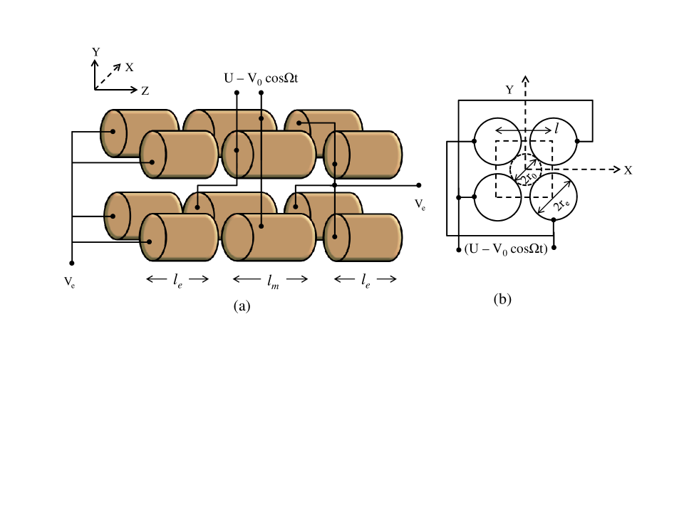
Figure 1: (a) Schematic of the linear ion trap used in the experiment. (b) End view of the four middle electrodes with relevant electrical connections. Various dimensions as marked by $l_{e}$, $l_{m}$, $l$, $r_{e}$ and $r_{0}$ are described in section 3.

These equations (eqn. 2) can be rewritten as

$$\frac{d^{2}u}{d\zeta^{2}}+(a_{u}-2q_{u}\cos 2\zeta)u=0,$$ (3)

with $u=x,y$, where

$$a_{x} = -a_{y}=\frac{4eU}{mr_{0}^{2}\Omega^{2}},$$

$$q_{x} = -q_{y}=\frac{2eV_{0}}{mr_{0}^{2}\Omega^{2}},$$ (4)

and $\zeta=\Omega t/2$. Eqn. 3 is standard Matheiu differential equation and its solution provides stability or instability of the ion motion [11] depending on the values of the parameters $a$ and $q$ as defined in eqn. 2. There exists a region in $a$ vs. $q$ diagram for which the ion-motion is stable along a particular direction, for example along $x$. A similar stability region exists for the motion along $y$ direction. An intersection between these two stability regions thus signifies a stable motion in $xy$ plane. For stable ion motion the trap should be operated at $q<0.908$.

The stable solutions of Mathieu differential equation show that the trapped ion oscillates with different frequencies given by [12]

$$\omega_{n}=\frac{(2n\pm\beta)\Omega}{2},n=0,1,2,3...$$ (5)

Here $\beta$ is a function of the trap operating parameters $a$, $q$ and for their small values, $\beta=\sqrt{a+q^{2}/2}$. The fundamental frequency $\omega_{0}$ (that corresponds to $n=0$) of secular motion and other micromotion frequencies are given by

$$\omega_{0} = \frac{\beta\Omega}{2},$$ (6)

$$\omega_{1\pm} = \Omega\pm\omega_{0},$$

$$\omega_{2\pm} = \Omega\pm 2\omega_{0}$$

and so on. A large spectra of the motional frequency have been obtained in our experiment by using electric dipole excitation technique.

Though in ideal case the trap potential is quadrupolar, real traps appear with misalignment, defect in machining, truncation and holes in the electrodes to have optical access. In addition, there are space charge developed by the trapped ions themselves. All these result in deviation from pure quadrupole trap potential contributing to other higher order terms and make the ion motion unstable for certain values of the trapping parameters, for which the stability exists in ideal case. The ions gain energy from the rf trapping field and their motional amplitudes get enhanced resulting loss from the trap. The condition of such nonlinear resonances is given by [13]

$$n_{x}\omega_{0x}+n_{y}\omega_{0y}=\Omega,n_{x},n_{y}=0,1,2,3...$$ (7)

where $\omega_{0x}$ and $\omega_{0y}$ are the secular frequencies for the motion along $x$ and $y$ respectively. Here $n_{x}+n_{y}=k$ is the order of the multipole. If one of the trap parameters is varied, a parametric resonance appears at a definite value subjected to the condition defined by eqn. 7 and it gives rise to instabilities called “black canyons” [14] within the stability diagram.

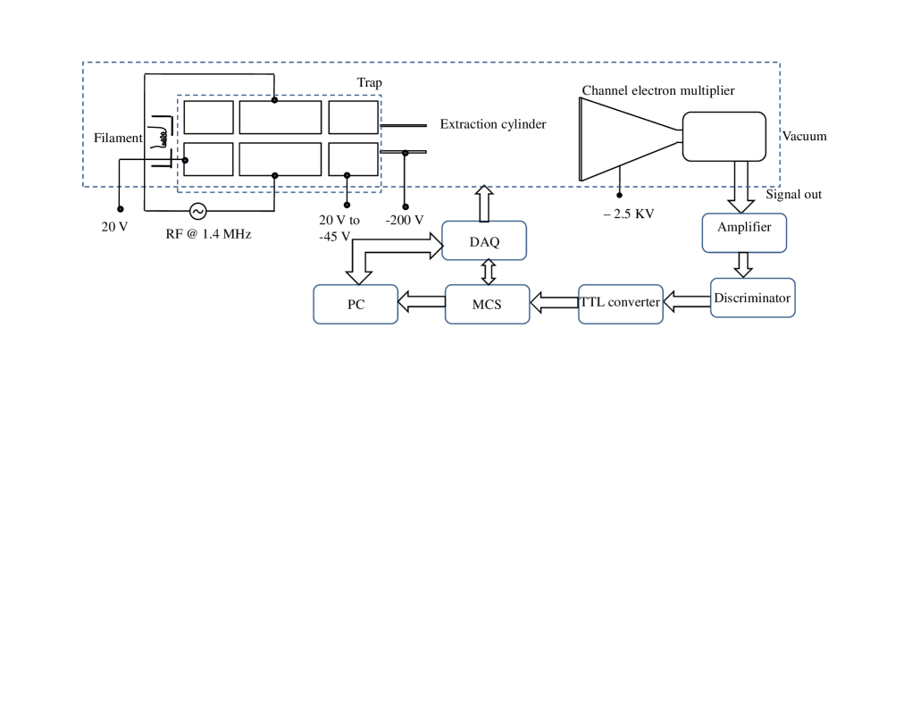
Figure 2: Schematic of the experimental setup. The trap, filament and the CEM with other ion optics (extraction cylinder) are housed in a vacuum chamber. The functioning and control of the signal processing devices are explained in the text.

3 Experimental setup

The schematic of the whole experimental setup is presented in figure 2. It consists of a linear Paul trap as shown in figure 1, an ionization setup, extraction and detection setup. The linear trap is assembled from four three-segmented electrodes each placed at four corners of a square of side ($l$) $12.73$ mm [figure 1](b). Each of twelve rods are of diameter ($2r_{e}$) $10$ mm. The four middle rods are of length ($l_{m}$) $25$ mm while all others are $15$ mm long ($l_{e}$) [figure 1(a)]. The separation between the surfaces of the diagonally opposite rods ($2r_{0}$) is $8$ mm. The middle electrode is separated from the end electrodes by a gap of $2$ mm. The molecular nitrogen ions (N${}_{2}^{+}$) are created by electron impact ionization. The ions are dynamically trapped for few hundreds ms before they are extracted by lowering the axial potential in one direction. The extracted ions are detected by a channel electron multiplier (CEM). The CEM produces one pulse corresponding to each ion and the pulse is successively processed through an amplifier, a discriminator, a TTL converter before it is fed into a multichannel scalar (MCS) card which ultimately counts the number of ions reaching the CEM. This time-of-flight (TOF) technique provides a detection efficiency around $10\%$. The time sequences are generated by National Instruments’ Data Acquisition (DAQ) hardware which is controlled by Labview and monitored by a personal computer (PC).

The trap is operated at a rf frequency of $1.415$ MHz and no dc potential is applied to the middle electrodes ($U=0$, $a_{u}=0$). The end electrodes are kept at $+20$ V while trapping. At the time of extraction, the end electrodes at the ion-exit-side are switched fast (within $75~{}ns$) from $+20$ V to $-45$ V.

4 Experimental results

Figure 3: Number of trapped ions ($N$) as a function of $q$ ($a=0$). Sudden fall of $N$ about some specific values of $q$ corresponds to nonlinear resonances as explained in the text. The numbers $6$, $7$, $8$ describe the order of the multipoles to which the resonances are assigned.

4.1 Stability characteristics

The stability behaviour of the trap is studied by varying the trap-operating-parameter $q$ while keeping the other parameter $a$ at zero. The $q$ is varied in steps of $0.0008$ by changing the rf amplitude at small intervals of $0.35$ V while the number of trapped ions ($N$) is plotted in figure 3 as a function of $q$. It shows that $N$ grows with $q$ initially but decreases above $q\approx 0.5$. It remains almost constant and shows a plateau for $0.3<q<0.5$. The q scanning is restricted to $0.6$ due to the presence of heavier masses which can not be resolved in the TOF spectra.

One of the significant observations within this stability diagram is the appearance of narrow nonlinear resonances for specific values of $q$. These are due to the existence of higher order multipoles within the trap potential as explained in section 2. The resonances appear at $q=0.3461,0.4073$ and $0.4885$ are assigned to the $8$th,$7$th and $6$th order multipoles respectively. The $7$th order multipole is unlikely as the symmetry of trap setup forbids non-zero perturbations due to odd order multipole. However, such a nonlinear observation has been observed previously [15]. It could result from any misalignment of the setup that partially breaks the radial symmetry or due to some electrical connection wires near the trap center. The nonlinear resonance at $q=0.5163$ in our experiment could not be assigned. It may result from other atmospheric species, or some molecules produced by charge-transfer-reactions inside the trap. As can be seen from figure 3, the depth of the resonance appearing at $q=0.4885$ is maximum and hence it can be concluded that the $6$th order multipole is the strongest one in our trap setup.

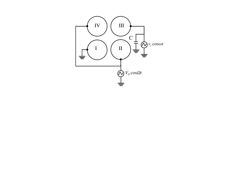
Figure 4: Schematic of the circuit used for dipole excitation of trapped ions. The dipole excitation signal $v_{i}\cos\omega t$ is applied between the electrodes marked as I and III.

While operating the trap for a single ion, the region of instabilities should be avoided as the ion gains energy from the time varying trapping field corresponding to these operating regions and its motional amplitude increases. It can add to systematics in precision measurement on the ion.

4.2 Dipole excitation of trapped ions

Electric dipole excitation of the trapped ions has been employed to measure their secular frequency and to obtain motional spectra. An electric dipole field has been applied on one of the middle electrodes as shown schematically in figure 4. The amplitude of the excitation potential ($v_{i}$) is kept fixed while its frequency is tuned so as to match with the secular frequency of the trapped ions. The trap operating parameters are kept fixed during the experiment. After the ions are loaded into the trap, the dipole excitation field is applied for few hundreds of ms. After a short waiting time, the ions are released and detected. The frequency of the excitation signal ($\omega$) is varied and the total number of ions is detected in each step.

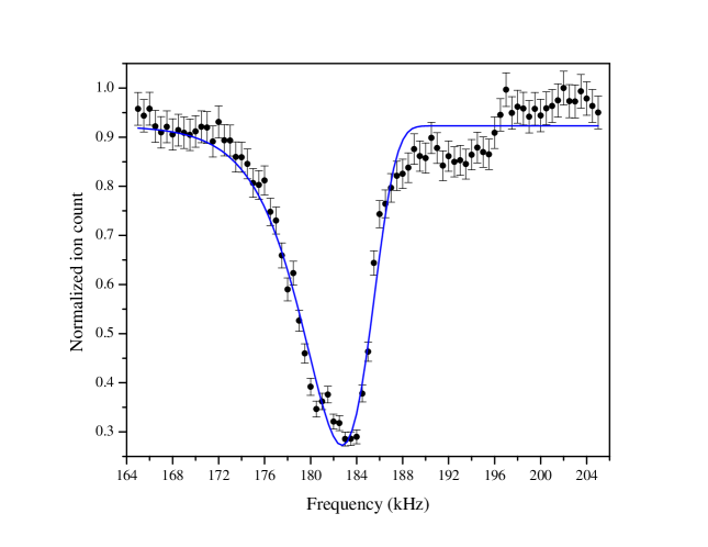
Figure 5: Dipole excitation resonance of trapped ions. Solid line shows a fit to the data with model function described in eqn. 8.

4.2.1 Measurement of secular frequency

The experimentally obtained ion counts ($N$) have been normalised after dividing by the maximum ion count ($N_{max}$) during a particular experiment. The normalised ion count ($N_{n}=N/N_{max}$) with associated uncertainty, has been plotted as a function of the frequency ($\omega/2\pi$) of the dipole excitation signal. Figure 5 shows such a dipole excitation resonance plot obtained with an excitation amplitude $v_{i}=50$ mV. The frequency is scanned from $165$ kHz to $205$ kHz in steps of $500$ Hz. The excitation signal is applied during $150$ ms in each step. The experimental data points have been fitted with the following function,

$$N_{n}=N_{0}+A\exp\left[-\exp(-\omega^{\prime})-\omega^{\prime}+1\right],$$ (8)

with $\omega^{\prime}=(\omega-\omega_{0})/\sigma$. Here $\omega_{0}$ is the resonant frequency and is equal to the secular frequency of the trapped ions. $N_{0}$ is an offset, $A$ is a scaling factor and $\sigma$ is the full-width at half-maxima (FWHM) of the resonance. The secular frequency of the trapped ions obtained from the fit is $182.730$($76$) kHz and it is in good agreement with theoretically calculated value.

4.2.2 Motional spectra

The motional spectra of the trapped ions as described in section 2 have been measured by varying the dipole excitation signal frequency over long range. Figure 6 shows the motional spectra in the radial plane. The fundamental or the first harmonic frequency of oscillation is observed at $\omega_{0}=2\pi\times 184$ kHz that corresponds to the trap operating parameter $a=0$, $q=0.39$ and it is the strongest one. The second and third harmonics are observed at $386$ kHz and $577$ kHz respectively. The other motional spectra as described in eqn. 6 are observed at $\omega_{2-}=2\pi\times 915$ kHz, $\omega_{1-}=2\pi\times 1.109$ MHz, $\omega_{1+}=2\pi\times 1.492$ kHz and $\omega_{2+}=2\pi\times 1.685$ MHz.

Figure 6: The normalized ion count $N$ plotted as a function of the dipole excitation frequency (in kHz) presenting the motional spectra of the trapped ion cloud. The amplitude of the excitation voltage is $v_{i}=100$ mV and the trap operating parameters are set at $a=0$, $q=0.39$ for N${}_{2}^{+}$. The frequency of the trap supply voltage is $\Omega=2\pi\times 1.3$ MHz.

4.2.3 Application

The accurate measurement of the motional frequency of the trapped ions is essential for different studies on them [16]. In a real linear Paul trap the radial motion is coupled with the axial motion and hence a variation in the axial potential affects the secular frequency of the ions [15]. The motional frequency of the trapped ions for different axial potentials has been measured with the technique described in section 4.2.1 and from this measurement the geometrical radial-axial coupling constant has been determined. This is important for any precision spectroscopic study on a single ion confined in this setup. The dipole excitation technique is also applied to study the shift in the motional frequency due to space charge created by the trapped ions. It is observed that the frequency decreases while they oscillate collectively with increasing space charge [17]. Detailed discussion on these topics can be found elsewhere [16, 17].

5 Conclusions

This colloquium paper describes the development of an ion trap facility at IACS and the results of some experiments fundamentally based on the dynamics of a trapped ion cloud. It presents a demonstration of some first principles of ion-trap-physics that are of common interest to an audience coming from wide variety of physics and participating in this colloquium. The results are also some significant feeds to the precision measurement based on a single ion in a linear Paul trap.

6 Acknowledgement

The authors thank S. Das, D. De Munshi and T. Dutta, presently at the Centre for Quantum Technologies, National University of Singapore, for their support in developing the experimental setup at IACS, and beyond it. The machining support from Max-Planck Institute, Germany is gratefully acknowledged.

References

- [1] H Dehmelt Physica Scripta T22 102 (1988)
- [2] R S Van Dyck, P B Schwinberg and H G Dehmelt Phys. Rev. Lett. 59 26 (1987)
- [3] N Yu, W Nagourney and H Dehmelt Phys. Rev. Lett. 78 4898 (1997)
- [4] G P Barwood et al. Phys. Rev. Lett. 93 133001 (2004)
- [5] W H Oskay et al. Phys. Rev. Lett. 94 163001 (2005)
- [6] C F Roos et al. Nature 443 316 (2006)
- [7] N Fortson Phys. Rev. Lett. 70 2383(1993)
- [8] P Mandal and M Mukherjee Phys. Rev. A 82 050101(R) (2010)
- [9] B K Sahoo, P Mandal and M Mukherjee Phys. Rev. A 83 030502(R) (2011)
- [10] O O Versolato et al. Phys. Rev. A 82 010501(R) (2010)
- [11] P H Dawson Quadrupole Mass Spectrometry and Its Applications Elsevier (1976)
- [12] P K Ghosh Ion Traps Oxford University Press (1995)
- [13] P H Dawson and N R Whetten Int. J. Mass Spectrom. Ion Phys. 2 45 (1969)
- [14] R E March and J F J Todd Quadrupole Ion Trap Mass Spectrometry John Wiley & Sons (2005)
- [15] A Drakoudis, M Söllner and G Werth Int. J. Mass Spectrom. 252 61 (2006)
- [16] P. Mandal PhD Thesis University of Calcutta submitted (2013)
- [17] P. Mandal et al. arXiv 1305.7081v1 [physics-atom-ph] (2013)