UdeM-GPP-TH-13-225

Measurement of $\gamma$ using $B\to K\pi\pi$ and $B\to KK{\overline{K}}$ decays

Bhubanjyoti Bhattacharya, David London

Physique des Particules, Université de Montréal,
C.P. 6128, succ. centre-ville, Montréal, QC, Canada H3C 3J7

and

Maxime Imbeault

Département de physique, Cégep de Saint-Laurent,
625, avenue Sainte-Croix, Montréal, QC, Canada H4L 3X7

The BaBar measurements of the Dalitz plots for $B^{0}\to K^{+}\pi^{0}\pi^{-}$, $B^{0}\to K^{0}\pi^{+}\pi^{-}$, $B^{+}\to K^{+}\pi^{+}\pi^{-}$, $B^{0}\to K^{+}K^{0}K^{-}$, and $B^{0}\to K^{0}K^{0}{\overline{K}}^{0}$ decays are used to cleanly extract the weak phase $\gamma$. We find four possible solutions: $(31^{+2}_{-3})^{\circ}$, $(77\pm 3)^{\circ}$, $(258^{+4}_{-3})^{\circ}$, and $(315^{+3}_{-2})^{\circ}$. One solution – $(77\pm 3)^{\circ}$ – is consistent with the SM. Its error, which includes leading-order flavor-SU(3) breaking, is far smaller than that obtained using two-body $B$ decays.

Talk given by David London at the 2013 Flavor Physics and CP Violation conference (FPCP-2013), Buzios, Rio de Janeiro, Brazil, May 19-24, 2013.
Talk based on arXiv:1303.0846 [1].

The standard way to obtain clean information about CKM phases is through the measurement of indirect CP violation in $B^{0}/{\overline{B}}^{0}\to f$. The conventional wisdom is that one cannot obtain such clean information from 3-body decays. There are two reasons. First, $f$ must be a CP eigenstate. While this holds for certain 2-body final states (e.g., $J/\psi K_{S}$, $\pi^{+}\pi^{-}$, etc.), 3-body states are, in general, not CP eigenstates. For example, consider $K_{S}\pi^{+}\pi^{-}$: the value of its CP depends on whether the relative $\pi^{+}\pi^{-}$ angular momentum is even (CP $+$) or odd (CP $-$). Second, one can only cleanly extract a weak phase using indirect CP asymmetries if the decay is dominated by amplitudes with a single weak phase. But 3-body decays generally receive significant contributions from amplitudes with different weak phases. Even if the CP of the 3-body final state could be fixed in some way, we would still need a way of dealing with this “pollution.”

Recently it was shown that all of these difficulties can be overcome [2, 3, 4]. There are three ingredients. First, the Dalitz plots of the 3-body decays are used to separate CP $+$ and CP $-$ final states. Second, the decay amplitudes are expressed in terms of diagrams. This permits the removal of the above pollution. Third, the electroweak-penguin (EWP) and tree diagrams are related, which reduces the number of unknown parameters. These three points are discussed below.

In the decay $B\to P_{1}P_{2}P_{3}$, one defines the three Mandelstam variables $s_{ij}\equiv\left(p_{i}+p_{j}\right)^{2}$, where $p_{i}$ is the momentum of $P_{i}$. (The three $s_{ij}$ are not independent, but obey $s_{12}+s_{13}+s_{23}=m_{B}^{2}+m_{1}^{2}+m_{2}^{2}+m_{3}^{2}$.) The Dalitz plot is given in terms of two Mandelstam variables, say $s_{12}$ and $s_{13}$. The key point is that, using the Dalitz plot, one can reconstruct the full decay amplitude ${\cal M}(B\to P_{1}P_{2}P_{3})(s_{12},s_{13})$.

The amplitude for a state with a given symmetry is then found by applying this symmetry to ${\cal M}(s_{12},s_{13})$. For example, the amplitude for the final state $K_{S}\pi^{+}\pi^{-}$ with CP $+$ is symmetric in $2\leftrightarrow 3$. This is given by $[{\cal M}(s_{12},s_{13})+{\cal M}(s_{13},s_{12})]/\sqrt{2}$. This amplitude is then used to compute all the observables for the decay. Note: all observables are momentum dependent – they take different values at each point in the Dalitz plot.

In order to remove the pollution due to additional decay amplitudes, one first expresses the full amplitude in terms of diagrams [2]. These are similar to those of two-body $B$ decays ($T$, $C$, etc.), but here one has to “pop” a quark pair from the vacuum. We add the subscript “1” (“2”) if the popped quark pair is between two non-spectator final-state quarks (two final-state quarks including the spectator). Fig. 1 shows the $T^{\prime}_{1}$ and $T^{\prime}_{2}$ diagrams contributing to $B\to K\pi\pi$ (as this is a ${\overline{b}}\to{\overline{s}}$ transition, the diagrams are written with primes).

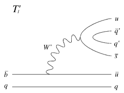
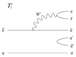
Figure 1: $T^{\prime}_{1}$ and $T^{\prime}_{2}$ diagrams contributing to $B\to K\pi\pi$.

Note: unlike the 2-body diagrams, the 3-body diagrams are momentum dependent. This must be taken into account whenever the diagrams are used.

In $B\to K\pi$ decays, under flavor SU(3) symmetry there are relations between the EWP and tree diagrams [5]. In Ref. [3] it was shown that similar EWP-tree relations hold for $B\to K\pi\pi$ decays. Taking $c_{1}/c_{2}=c_{9}/c_{10}$ for the Wilson coefficients (which holds to about 5%), these take the simple form (the exact relations are given in Ref. [3])

$$P^{\prime}_{EWi}=\kappa T^{\prime}_{i}~{}~{},~{}~{}~{}~{}P^{\prime C}_{EWi}=\kappa C^{\prime}_{i}~{}~{}~{}~{}(i=1,2)~{},$$ (1)

where

$$\kappa\equiv-\frac{3}{2}\frac{|\lambda_{t}^{(s)}|}{|\lambda_{u}^{(s)}|}\frac{c_{9}+c_{10}}{c_{1}+c_{2}}~{},$$ (2)

with $\lambda_{p}^{(s)}=V^{*}_{pb}V_{ps}$.

However, there is an important caveat. Under SU(3), the final state in $B\to K\pi\pi$ involves three identical particles, so that the six permutations of these particles must be taken into account. But the EWP-tree relations hold only for the totally symmetric state. This state, ${\cal M}_{\rm fs}$ (‘fs’ = ‘fully symmetric’), is found by symmetrizing ${\cal M}(s_{12},s_{13})$ under all permutations of 1,2,3. The analysis must therefore be carried out for this state.

With the above three ingredients, one can cleanly extract weak-phase information from 3-body decays. The fundamental idea is as follows. It is common to combine observables from different 2-body $B$ decays in order to extract weak-phase information. Examples include obtaining $\alpha$ from $B\to\pi\pi$ [6], obtaining $\gamma$ from $B\to DK$ [7, 8, 9], and observing the “$B\to\pi K$ puzzle” in $B\to\pi K$ [10]. In 3-body $B$ decays, the idea is the same, except that the analysis applies to each point in the Dalitz plot. (That is, the analysis is momentum dependent.) The disadvantage is that the analysis is more complicated. However, there is a big advantage: since it holds at each point in the Dalitz plot, the analysis really represents many independent determinations of the weak-phase information. These can be combined, considerably reducing the error. Below we present an example of such an analysis involving $B\to K\pi\pi$ and $B\to KK{\overline{K}}$ decays [4].

We consider the five decays $B^{0}\to K^{+}\pi^{0}\pi^{-}$, $B^{0}\to K^{0}\pi^{+}\pi^{-}$, $B^{+}\to K^{+}\pi^{+}\pi^{-}$, $B^{0}\to K^{+}K^{0}K^{-}$, and $B^{0}\to K^{0}K^{0}{{\overline{K}}^{0}}$. The $B\to K\pi\pi$ amplitudes are written in terms of diagrams with a popped $u{\overline{u}}$ or $d{\overline{d}}$ quark pair (these are equal under isospin), while the diagrams of the $B\to KK{\overline{K}}$ amplitudes have a popped $s{\overline{s}}$ pair. But flavor-SU(3) symmetry, which is needed for the EWP-relations, implies that all diagrams are equal. All five amplitudes are therefore written in terms of the same diagrams.

Note, however, that flavor-SU(3) symmetry is not exact. It is therefore important to keep track of a possible difference between $B\to K\pi\pi$ and $B\to KK{\overline{K}}$ decays.

The expressions for the amplitudes in terms of diagrams are given in Ref. [4]. The diagrams can be combined into “effective diagrams” [1]:

$$a\equiv-{\tilde{P}}^{\prime}_{tc}+\kappa\left(\frac{2}{3}T^{\prime}_{1}+\frac{1}{3}C^{\prime}_{1}+\frac{1}{3}C^{\prime}_{2}\right)~{},~{}~{}~{}$$

$$b\equiv T^{\prime}_{1}+C^{\prime}_{2}~{},~{}~{}c\equiv T^{\prime}_{2}+C^{\prime}_{1}~{},~{}~{}d\equiv T^{\prime}_{1}+C^{\prime}_{1}~{}.$$ (3)

The decay amplitudes can now be written in terms of five diagrams, $a$-$d$ and ${\tilde{P}}^{\prime}_{uc}$:

$$2A(B^{0}\to K^{+}\pi^{0}\pi^{-})_{\rm fs} = be^{i\gamma}-\kappa c~{},$$

$$\sqrt{2}A(B^{0}\to K^{0}\pi^{+}\pi^{-})_{\rm fs} = -de^{i\gamma}-{\tilde{P}}^{\prime}_{uc}e^{i\gamma}-a+\kappa d~{},$$

$$\sqrt{2}A(B^{+}\to K^{+}\pi^{+}\pi^{-})_{\rm fs} = -ce^{i\gamma}-{\tilde{P}}^{\prime}_{uc}e^{i\gamma}-a+\kappa b~{},$$

$$\sqrt{2}A(B^{0}\to K^{+}K^{0}K^{-})_{\rm fs} = \alpha_{SU(3)}(-ce^{i\gamma}-{\tilde{P}}^{\prime}_{uc}e^{i\gamma}-a+\kappa b)~{},$$

$$A(B^{0}\to K^{0}K^{0}{{\overline{K}}^{0}})_{\rm fs} = \alpha_{SU(3)}({\tilde{P}}^{\prime}_{uc}e^{i\gamma}+a)~{}.$$ (4)

In the above, $\alpha_{SU(3)}$ measures the amount of flavor-SU(3) breaking between $B\to K\pi\pi$ and $B\to KK{\overline{K}}$ decays, i.e., between diagrams with a final-state $u{\overline{u}}$/$d{\overline{d}}$ quark pair and those with an $s{\overline{s}}$ pair. It must be stressed that $\alpha_{SU(3)}$ is only a leading-order SU(3)-breaking term. For example, it assumes that the SU(3) breaking is the same for all diagrams. The possible effect of next-to-leading-order SU(3) breaking must be kept in mind.

Now, in the flavor-SU(3) limit, $\alpha_{SU(3)}=1$ (the imaginary piece vanishes in this limit), so that we have $A(B^{+}\to K^{+}\pi^{+}\pi^{-})_{\rm fs}=A(B^{0}\to K^{+}K^{0}K^{-})_{\rm fs}$. This implies that the $B^{+}$ decay does not furnish any new information. The remaining four amplitudes depend on 10 theoretical parameters: 5 magnitudes of diagrams, 4 relative phases, and $\gamma$. But there are 11 experimental observables: the decay rates and direct asymmetries of each of the 4 processes, and the indirect asymmetries of $B^{0}\to K^{0}\pi^{+}\pi^{-}$, $B^{0}\to K^{+}K^{0}K^{-}$ and $B^{0}\to K^{0}K^{0}{{\overline{K}}^{0}}$. With more observables than theoretical parameters, $\gamma$ can be extracted from a fit.

If one allows for SU(3) breaking ($|\alpha_{SU(3)}|\neq 1$), we can add two more observables: the decay rate and direct CP asymmetry for the $B^{+}$ decay. In this case it is possible to extract $\gamma$ even with the inclusion of $|\alpha_{SU(3)}|$ as a fit parameter. (Note that the observables are insensitive to the phase of $\alpha_{SU(3)}$.)

Since the diagrams and observables are all momentum dependent, this implies that the above method for extracting $\gamma$ in fact applies to each point in the Dalitz plot. However, since the value of $\gamma$ is independent of momentum, the method really represents many independent measurements of $\gamma$. These can be combined, reducing the error on $\gamma$.

The observables are obtained as follows. The $B\to P_{1}P_{2}P_{3}$ amplitude is written as

$${\cal M}(s_{12},s_{13})={\cal N}_{\rm DP}\sum\limits_{j}c_{j}e^{i\theta_{j}}F_{j}(s_{12},s_{13})~{},$$ (5)

where the index $j$ runs over all resonant and non-resonant contributions. Each contribution is expressed in terms of isobar coefficients $c_{j}$ (amplitude) and $\theta_{j}$ (phase), and a dynamical wave function $F_{j}$. The $F_{j}$ take different forms depending on the contribution. The $c_{j}$ and $\theta_{j}$ are extracted from a fit to the Dalitz-plot event distribution.

BaBar has performed such fits for the five decays of interest [11]. For each decay, given the $c_{j}$, $\theta_{j}$ and $F_{j}$, we reconstruct the amplitude for that decay as a function of $s_{12}$ and $s_{13}$. We then obtain ${\cal M}_{\rm fs}$ by symmetrizing under all permutations of 1,2,3. This process is repeated for the CP-conjugate process, where we construct $\overline{{\cal M}}_{\rm fs}$.

The experimental observables are then obtained as follows:

$$X(s_{12},s_{13}) = |{\cal M}_{\rm fs}(s_{12},s_{13})|^{2}+|\overline{{\cal M}}_{\rm fs}(s_{12},s_{13})|^{2}~{},$$

$$Y(s_{12},s_{13}) = |{\cal M}_{\rm fs}(s_{12},s_{13})|^{2}-|\overline{{\cal M}}_{\rm fs}(s_{12},s_{13})|^{2}~{},$$

$$Z(s_{12},s_{13}) = {\rm Im}\left[{\cal M}^{*}_{\rm fs}(s_{12},s_{13})~{}\overline{{\cal M}}_{\rm fs}(s_{12},s_{13})\right]~{}.$$ (6)

The experimental error bars on these quantities are found by varying the input isobar coefficients over their $1\sigma$-allowed ranges. The effective CP-averaged branching ratio ($X$), direct CP asymmetry ($Y$), and indirect CP asymmetry ($Z$) may be constructed for every point on any Dalitz plot. However, $Z$ can be measured only for $B^{0}$ decays to a CP eigenstate.

There is one technical point: in its $K_{S}K_{S}K_{S}$ analysis, due to limited statistics BaBar takes $A(B^{0}\to K_{S}K_{S}K_{S})=A({\overline{B}}^{0}\to K_{S}K_{S}K_{S})$. This implies that (i) $Y$ and $Z$ vanish for every point of the Dalitz plot, and (ii) the (small) diagram ${\tilde{P}}^{\prime}_{uc}$ must be set to zero. The removal of an equal number of unknown parameters (amplitude and phase of ${\tilde{P}}^{\prime}_{uc}$) and observables does not affect the viability of the method.

Since the amplitudes used to construct the observables are fully symmetric under the interchange of the three Mandelstam variables, only one sixth of the Dalitz plot provides independent information. In order to avoid multiple counting, we divide each Dalitz plot into six zones by its three axes of symmetry, and use information only from one zone. This is illustrated in Fig. 2, which shows the kinematic boundaries and symmetry axes of the $B\to K\pi\pi$ and $B\to KK{\overline{K}}$ Dalitz plots. The 50 points in the region of overlap of the first of six zones from all Dalitz plots are used for the $\gamma$ measurement.

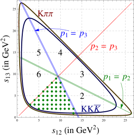
Figure 2: Kinematic boundaries and symmetry axes of the $B\to K\pi\pi$ and $B\to KK{\overline{K}}$ Dalitz plots. The symmetry axes divide each plot into six zones.

We now perform a maximum likelihood analysis for extracting $\gamma$. For each of the 50 points in the first Dalitz-plot zone, we construct the $-2\Delta\ln{\rm L}(\gamma)$ function, where ${\rm L}$ represents the likelihood. The sum of such functions over all fifty points gives us a joint likelihood distribution. The local minima of this function are then identified as the most-likely values of $\gamma$. In order to find the $1\sigma$ error bar on $\gamma$ we first shift the likelihood function along the vertical axis so that the zero of the function corresponds to a local minimum. We then look for the range of $\gamma$ that results in a unit shift along the vertical axis of the $-2\Delta\ln{\rm L}(\gamma)$ vs $\gamma$ plot. The $1\sigma$ error bars on $\gamma$ are given by the condition that $\Delta(-2\Delta\ln{\rm L}(\gamma))=1$.

We perform 3 types of fit:

1. We assume that flavor SU(3) is a good symmetry, so that $\alpha_{SU(3)}=1$. The fit involves only the four $B^{0}$ decay channels.

2. SU(3) breaking is allowed and treated as follows. The ratio of $X$’s is constructed point by point from the Dalitz plots for $B^{+}\to K^{+}\pi^{+}\pi^{-}$ and $B^{0}\to K^{+}K^{0}K^{-}$, giving $|\alpha_{SU(3)}|^{2}(s_{12},s_{13})$. We use $|\alpha_{SU(3)}|$ found in this way to correct the observables from the $B\to KK{\overline{K}}$ Dalitz plots and use the corrected numbers in a new maximum-likelihood analysis for finding $\gamma$.

3. We consider observables from all five Dalitz plots but now include $|\alpha_{SU(3)}|$ as an additional unknown hadronic parameter.

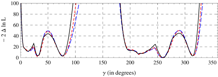
Figure 3: Results of maximum-likelihood fits. The solid (black) curve represents the fit assuming flavor-SU(3) symmetry. The short dashes (red) represent the fit where flavor-SU(3) breaking is fixed by a point-by-point comparison of Dalitz plots for $B^{+}\to K^{+}\pi^{+}\pi^{-}$ and $B^{0}\to K^{+}K^{0}K^{-}$. The long dashes (blue) represent the fit with inputs from five Dalitz plots and an extra hadronic fit parameter $|\alpha_{SU(3)}|$.

The results of the maximum-likelihood fits are shown in Fig. 3. From this figure, we see that there is very little difference among the three fits. This shows that, on average, SU(3) breaking is small. This is consistent with the result from fit 2: averaged over the 50 points, we find that $|\alpha_{SU(3)}|=0.97\pm 0.05$ (recall that $\alpha_{SU(3)}=1$ corresponds to no SU(3) breaking).

There are four preferred values for $\gamma$:

$$(31^{+2}_{-3})^{\circ}~{}~{},~{}~{}~{}~{}(77\pm 3)^{\circ}~{}~{},~{}~{}~{}~{}(258^{+4}_{-3})^{\circ}~{}~{},~{}~{}~{}~{}(315^{+3}_{-2})^{\circ}~{}.$$ (7)

Three of these indicate new physics (is this a “$K\pi\pi$-$KK{\overline{K}}$ puzzle”?), but one solution – $(77\pm 3)^{\circ}$ – is consistent with the standard model.

In all cases, the error is small, 2-4^∘. This can be understood as follows. The key point is that this method really involves 50 independent measurements of $\gamma$. Roughly speaking, if each measurement has an error of $\pm 20^{\circ}$, which is somewhat larger than other methods, then when we take a naive average, we divide the error by $\sqrt{50}$, giving a final error of $\sim 3^{\circ}$.

There are several potential sources of error that have not been included in our method. The first is correlations. Although the errors on the isobar coefficients extracted from a given Dalitz plot are in general correlated, such information is not always publicly available. In our analysis we have considered the errors to be completely uncorrelated, but we hope that a future analysis by an experimental collaboration will take such effects into account.

Second there are possible effects from higher-order flavor-SU(3) breaking. Such breaking may arise due to the nonzero mass difference between pions and kaons, and between intermediate resonances. Indeed, after the talk, Yuval Grossman expressed some skepticism about having only one SU(3)-breaking parameter, and asked if it were possible to include more. Unfortunately, this cannot be done. In the method, there are 11 observables and 9 unknown parameters (these include $|\alpha_{SU(3)}|$). If a second SU(3)-breaking parameter were added, there would then be 11 unknowns (these include the two magnitudes and the relative phase of the SU(3)-breaking parameters). In this case, with an equal number of observables and unknown parameters, one could still extract $\gamma$, but only with even more discrete ambiguities.

This said, the error due to leading-order SU(3) breaking is small, and so it is unlikely that the error due to higher-order SU(3) breaking is larger. We can get a bit of a handle on this as follows. As mentioned above, in fit 2 one obtains $|\alpha_{SU(3)}|^{2}(s_{12},s_{13})$ by computing, point by point, the ratio of $X$’s in the $B^{+}\to K^{+}\pi^{+}\pi^{-}$ and $B^{0}\to K^{+}K^{0}K^{-}$ Dalitz plots. These are then averaged over all 50 points, giving the average value of leading-order SU(3) breaking $|\alpha_{SU(3)}|=0.97\pm 0.05$. In fact, this can be done in two different ways. One can compare the $|{\cal M}_{\rm fs}(s_{12},s_{13})|^{2}=(X+Y)/2$ of the two Dalitz plots to obtain (when averaged) $|\alpha_{SU(3)}^{\cal M}|$. Alternatively, one can compare the $|\overline{{\cal M}}_{\rm fs}(s_{12},s_{13})|^{2}=(X-Y)/2$, giving $|\alpha_{SU(3)}^{\overline{\cal M}}|$. To leading order, we expect $|\alpha_{SU(3)}^{\cal M}|=|\alpha_{SU(3)}^{\overline{\cal M}}|$, so that their difference indicates the size of higher-order SU(3) breaking. We find $|\alpha_{SU(3)}^{\cal M}|=0.97\pm 0.04$ and $|\alpha_{SU(3)}^{\overline{\cal M}}|=0.99\pm 0.04$, yielding a difference of $0.02\pm 0.06$. Though not a proof that higher-order SU(3) breaking is small, the smallness of this difference does suggest this conclusion.

Finally, there is one very important caveat, related to an error that has not been included, and that can significantly affect our result. All errors considered so far have been entirely statistical (even SU(3) breaking). But there is also the systematic, model-dependent error associated with the isobar analysis. This cannot be treated statistically, i.e., reduced by averaging. This error was not given in the BaBar papers and so we could not include it. Hopefully, the experimentalists themselves will redo this analysis, including all errors.

Recall that the standard way to directly probe $\gamma$ is via $B^{\pm}\to DK^{\pm}$ decays [7, 8, 9]. Although the two-body method is expected to be theoretically clean, it is difficult experimentally, so that the present direct measurement has a large error: $\gamma=(66\pm 12)^{\circ}$ [12]. The statistical error of 2-4^∘ in the three-body method is far smaller than the two-body error. If the systematic error is not too large, the three-body method could well be the best way to measure $\gamma$.

To summarize: about 2-3 years ago, it was shown that, theoretically, it is possible to cleanly extract weak-phase information from 3-body $B$ decays. In the present study, we demonstrate that this is, in fact, true. Using real data from BaBar, we extract the phase $\gamma$ from $B\to K\pi\pi$ and $B\to KK{\overline{K}}$ decays. We find that there is a fourfold discrete ambiguity, giving the preferred values $\gamma=31^{\circ}$, $77^{\circ}$, $258^{\circ}$ or $315^{\circ}$. However, in all cases, the error is small, 2-4^∘, and includes leading-order SU(3) breaking. This is due to the fact that, in this method, there are actually 50 independent measurements of $\gamma$. When these are combined, the error is considerably reduced.

The main thing that is missing is the systematic, model-dependent error related to the isobar Dalitz-plot analysis. It is only the experimentalists themselves who can properly include it. If the systematic error is not too large, then this 3-body method will likely be the best one for measuring $\gamma$.

ACKNOWLEDGEMENTS

A special thank you goes to E. Ben-Haim for his important input to this project. We also thank J. Charles, M. Gronau, N. Rey-Le Lorier, J. Rosner, J. Smith, Y. Grossman and A. Soffer for helpful communications. BB would like to thank G. Bell and WG IV of CKM 2012.

References

- [1] B. Bhattacharya, M. Imbeault and D. London, arXiv:1303.0846 [hep-ph].
- [2] N. Rey-Le Lorier, M. Imbeault and D. London, Phys. Rev. D 84, 034040 (2011) [arXiv:1011.4972 [hep-ph]].
- [3] M. Imbeault, N. Rey-Le Lorier and D. London, Phys. Rev. D 84, 034041 (2011) [arXiv:1011.4973 [hep-ph]].
- [4] N. Rey-Le Lorier and D. London, Phys. Rev. D 85, 016010 (2012) [arXiv:1109.0881 [hep-ph]].
- [5] M. Neubert and J. L. Rosner, Phys. Lett. B 441, 403 (1998) [arXiv:hep-ph/9808493], Phys. Lett. B 441, 403 (1998) [arXiv:hep-ph/9808493]; M. Gronau, D. Pirjol and T. M. Yan, Phys. Rev. D 60, 034021 (1999) [Erratum-ibid. D 69, 119901 (2004)] [arXiv:hep-ph/9810482].
- [6] M. Gronau and D. London, Phys. Rev. Lett. 65, 3381 (1990).
- [7] M. Gronau and D. London, Phys. Lett. B 253, 483 (1991); M. Gronau and D. Wyler, Phys. Lett. B 265, 172 (1991).
- [8] D. Atwood, I. Dunietz and A. Soni, Phys. Rev. Lett. 78, 3257 (1997) [hep-ph/9612433], Phys. Rev. D 63, 036005 (2001) [hep-ph/0008090].
- [9] A. Giri, Y. Grossman, A. Soffer and J. Zupan, Phys. Rev. D 68, 054018 (2003) [hep-ph/0303187].
- [10] For example, see A. J. Buras, R. Fleischer, S. Recksiegel and F. Schwab, Phys. Rev. Lett. 92, 101804 (2004) [hep-ph/0312259], PoS HEP 2005, 193 (2006) [hep-ph/0512059]; S. Baek and D. London, Phys. Lett. B 653, 249 (2007) [hep-ph/0701181]; S. Baek, C. -W. Chiang and D. London, Phys. Lett. B 675, 59 (2009) [arXiv:0903.3086 [hep-ph]].
- [11] : J. P. Lees et al. [BABAR Collaboration], Phys. Rev. D 83, 112010 (2011) [arXiv:1105.0125 [hep-ex]]; : B. Aubert et al. [BABAR Collaboration], Phys. Rev. D 80, 112001 (2009) [arXiv:0905.3615 [hep-ex]]; : B. Aubert et al. [BABAR Collaboration], Phys. Rev. D 78, 012004 (2008) [arXiv:0803.4451 [hep-ex]]; : J. P. Lees et al. [BABAR Collaboration], Phys. Rev. D 85, 112010 (2012) [arXiv:1201.5897 [hep-ex]]; : J. P. Lees et al. [BABAR Collaboration], Phys. Rev. D 85, 054023 (2012) [arXiv:1111.3636 [hep-ex]].
- [12] J. Charles et al. [CKMfitter Group Collaboration], Eur. Phys. J. C 41, 1 (2005) [hep-ph/0406184], updated results and plots available at http://ckmfitter.in2p3.fr/.