A Post-Newtonian approach to black hole-fluid systems

Abstract

This work devises a formalism to obtain the equations of motion for a black hole-fluid configuration. Our approach is based on a Post-Newtonian expansion and adapted to scenarios where obtaining the relevant dynamics requires long time-scale evolutions. These systems are typically studied with Newtonian approaches, which have the advantage that larger time-steps can be employed than in full general-relativistic simulations, but have the downside that important physical effects are not accounted for. The formalism presented here provides a relatively straightforward way to incorporate those effects in existing implementations, up to 2.5PN order, with lower computational costs than fully relativistic simulations.

I Introduction

The interaction between black holes and matter in accreting systems is known to power emission across a wide spectrum, and provides the engine for exciting phenomena such as AGNs, blazars, quasars, etc. Systems where a black hole interacts with a localized matter distribution also lie at the heart of other interesting astrophysical processes. For instance, black hole-star systems can give rise to strong tidal interactions that might induce supernova-like events Rosswog et al. (2009); the disruption of stars by a supermassive black hole can trigger strong flares MacLeod et al. (2012); Bloom et al. (2011); Kasen and Ramirez-Ruiz (2010); Hayasaki et al. (2012); Stone and Loeb (2010); Zalamea et al. (2010); stellar-mass black holes interacting with a neutron star can be responsible for short gamma-ray bursts Piran et al. (2012); Metzger et al. (2010); etc. The upcoming close encounter of our own SgrA^∗ with a gas cloud (G2), expected for next year Gillessen:2011aa , will provide unprecedented opportunities to study a nearby example of such interactions.

The understanding of these systems requires dealing with diverse physics – gravity and matter at least – and therefore solving general relativistic hydrodynamic equations in dynamical, strongly gravitating scenarios. Due to the complex and non-linear character of the underlying equations, numerical simulations are required to make realistic headways into the problem. This task, however, is formally complicated by several issues. First, depending on the problem under consideration, vastly different scales are involved – star and black-hole sizes –, as well as, potentially, extremely long dynamical times. Second, the physical theories one has to employ – general relativity and relativistic hydrodynamics – are not only highly involved/non-linear, but also bring different characteristic timescales for propagating modes. In particular, general relativity dictates that gravitational degrees of freedom propagate at the speed of light, while hydrodynamic modes do so at the sound speed, which can be significantly lower. This implies, at a computational level, that a fully general-relativistic study is necessarily more costly than a non-relativistic one.

There exist, however, a class of problems where propagating gravitational effects are secondary, and the above-mentioned limitation can be dealt with by suitable approximations. A typical approach is to assume that gravitational effects are described by Newtonian gravity, where the gravitational field is determined via elliptic equations, which can be solved efficiently (e.g. multigrid1 ; multigrid2 ; multigrid3 ) once appropriate boundary conditions are specified. The only hyperbolic equations are then given by hydrodynamics and, as a consequence, the dynamical propagation speeds are given by the speed of sound, which allows considerably larger step-sizes to be adopted. Gravitational radiation reaction may then be approximately included by using the quadrupole formula or higher-order extensions of it (c.f. for instance Ref. r_instability ; Guillochon et al. (2009); Ruffert and Janka (2010); Price and Rosswog (2006)).

However, for scenarios involving a black hole – even when ignoring propagating modes –, this strategy must be modified to incorporate crucial features brought by general relativity, which cannot be ignored unless the star remains very far from the black hole through the whole regime of interest. A widely used approach to address this issue is to consider the gravitational potential sourced by the star, and add to it the so-called “Pacynski-Wiita” (PV) potential $V(r)=-GM/(r-2GM/c^{2})$ Paczyńsky and Wiita (1980). This method therefore amounts to a phenomenological modification to the Newtonian potential, and guarantees the presence of an innermost stable circular orbit (ISCO) Abramowicz (2009). The PV potential, however, does not depend on the black-hole spin, and thus cannot properly describe rotating black holes. Furthermore, even for non-spinning black holes, the ISCO has different orbital frequency and angular momentum than in a Schwarzschild spacetime, even though it lies at $r=6M$, as for a Schwarzchild spacetime in the usual areal coordinates. Various increasingly sophisticated suggestions have been presented to partially address these shortcomings (see e.g. Nowak and Wagoner (1991); Semerák and Karas (1999); Kluźniak and Lee (2002); Wegg:2012yx ; Tejeda:2013mva ) for non-spinning black holes. However, crucial features brought by the presence of a black hole are still not fully accounted for (e.g. gravitational redshift, frame-dragging, gravitational radiation, etc.) unless further ad-hoc ingredients are incorporated. Naturally, since strong observational evidence indicates that gravitational waves exist and carry energy and angular momentum away from the system, as well as that black holes possess a variety of spins (spanning the whole allowed range $cJ/(GM^{2})\leq 1$, see e.g. Ref. McClintock:2011zq ), a better treatment of black hole effects on matter is desirable.

In this work, motivated by the above observations, we describe a systematic approach to treat the problem starting from the correct description in full General Relativity, and introduce a post-Newtonian (PN) expansion to capture relativistic effects in a consistent manner. This goal, as we describe below, has been pursued by other authors – either via fully general relativistic or approximate methods – but the resulting approaches require significantly revamping/altering traditional astrophysics modeling strategies. We thus adopt an approach that is intimately tied with the traditional “Newtonian-route”, providing a systematic way to include further physical ingredients in a controlled expansion of the equations or, alternatively, to estimate errors in the existing approaches.

For context, we briefly review related work. For instance, Ref. BDS_hydro developed a formalism similar to ours, focusing on fluid systems only (i.e. without a black hole) in the Arnowitt-Deser-Misner (ADM) gauge, with leading-order dissipative effects, and conservative effects included at 1PN order (see also Ref. faye_higher_order_fluxes for an extension of this formalism to next-to-leading order in the dissipative sector). The numerical implementation of the formalism of Ref. BDS_hydro , performed in Refs. ayal ; Oohara_nakamura1 ; Oohara_nakamura2 , achieved promising results, but found difficulties to produce sufficiently massive stars to describe neutron stars rosswog_private . As we illustrate in this work, to deal with these difficulties higher-order approximations are required. An attempt in this direction was made by Ref. shibata , which performed a comprehensive study of the equations of PN hydrodynamics and radiation reaction (for fluid systems only, i.e. in the absence of a black hole) in the 3+1 formalism and with several gauge choices, through 2.5PN order.

Higher-order extensions are particularly easy to achieve in the harmonic gauge often used in PN calculations, but this gauge choice would yield a scheme involving hyperbolic equations with characteristics speeds given by the speed of light, already at low PN orders. Such behavior is undesirable for studying mildly dynamical spacetimes whose true dynamics is governed by the characteristic speeds of the fluid describing the matter content. Along these lines, a recently introduced formalism, partially related to ours, is that of Refs. kim1 ; kim2 , which essentially consists of solving the 1PN Einstein equations with a conformally flat ansatz for the metric. While this approach indeed gets rid of characteristics with light-speed propagation, it only accounts for some effects at 1PN.

A different approach to describe compact-object binaries is given by the effective-one-body formalism (EOB) BD99 , which attempts to accelerate the convergence of the PN dynamics by “resumming” it (both in the conservative BD99 ; DJS3PN ; BBL12 ; damour01 ; DJS ; BB10 ; BB11 ; nagar and dissipative DamourResummedWfms ; tagoshi sectors). While very successful at describing binary black holes (see e.g. Ref. taracchini for a recent comparison to full general-relativistic results) and more recently neutron-star binaries EOB_NS1 ; EOB_NS2 , the EOB is not suitable for describing black holes interacting with matter that is not in a compact configuration. Last, within the fully general relativistic regime a few options have been pursued to study related systems within reasonable computational efforts. For instance, in East:2013iwa a method to reduce the computational cost of implementing the full Einstein equations coupled to matter has recently been introduced. This method allows one to treat black hole-star binary systems where the backreaction on the black hole is sufficiently small. In another approach, to study stellar black hole-white dwarf systems a suitable rescaling of the equation of state was introduced to study a related, though computationally tractable, problem and then extrapolate results to the problem of interest Paschalidis:2010dh . Alternatively, focus has been placed in the interaction of white dwards with intermediate mass black holes so as to deal with comparable scales Shcherbakov:2012iv . However, even in this regime simulations could only track the system for relatively short times.

While keeping in mind these issues and options, we here develop an approach consisting of minimal modifications to Newtonian theory. This has the advantage that existing (thoroughly tested/highly sophisticated) implementations of hydrodynamics (for representative examples, see e.g. Ruffert and Janka (2010); Guillochon et al. (2009); 2013ApJ…767…25G ) in Newtonian theory could be easily modified to implement our approach. Alternatively, our approach can be used to evaluate the importance of the PN effects that are missing in Newtonian simulations, and therefore gauge their errors relative to a fully general-relativistic treatment.

This work is organized as follows. Section II describes our basic strategy for adapting the standard PN expansion to the purpose of describing a black hole interacting with a relativistic-fluid configuration. In sections III and IV we present the derivations of the equations to first and second PN order. Section V describes how gravitational waves are accounted for, and how their effect can be incorporated in the elliptic system determining the gravitational and fluid behavior. In section VI we describe how to account for the black hole presence, while in section VII we present a discussion of implementation choices, together with a few examples.

II Basic strategy

An analytic description of the two-body dynamics in General Relativity, dating back originally to Einstein’s calculation of the perihelion of Mercury mercury , is given by the PN approximation. The PN formalism is essentially an expansion in the ratio between the typical velocity of the system, $v$, and the speed of light (see Ref. Blanchet (2006) for a recent review). For a fluid system, the dynamics is known through order $(v/c)^{5}$ beyond Newtonian theory (i.e. through 2.5PN order) PNfluid1 ; PNfluid2 ; PNfluid3 . For a binary system of non-spinning black holes, the conservative dynamics is known through 3PN order Damour et al. (2001); Blanchet et al. (2004), while the gravitational-wave fluxes have been computed through 3.5PN order Blanchet et al. (2005); Kidder (2008); Blanchet et al. (2008) (i.e. through order $(v/c)^{7}$ beyond the quadrupole formula) and 3PN order Arun et al. (2009), respectively for a system of two non-spinning black holes on circular or eccentric orbits. The effect of the spins on the dynamics of compact-object (and in particular black-hole) binaries has also been calculated, both in the conservative and dissipative sectors Blanchet et al. (2006); Blanchet et al. (2011a); Damour et al. (2008a); Steinhoff et al. (2008a, b); Hergt and Schäfer (2008); Hartung and Steinhoff (2011); Kidder (1995); Faye et al. (2006); Foffa and Sturani (2011); Porto et al. (2011); Porto and Rothstein (2006); Porto (2006); Porto and Rothstein (2008a, b); Porto (2010); Levi (2010, 2011).

One drawback of the PN expansion is that it is slowly convergent. As a result, the PN dynamics, if extrapolated to $v\sim c$, does not reproduce the correct general-relativistic dynamics accurately. This is particularly true for binary black-hole systems near coalescence. In fact, in order to obtain a sensible description of such systems in the strong field regime, the PN equations need to be “resummed” (i.e. completed by “educated guesses” of the higher-order terms in $v/c$, based on the known lower-order ones), both in the conservative BD99 ; DJS3PN ; BBL12 ; damour01 ; DJS ; BB10 ; BB11 ; nagar and dissipative DamourResummedWfms ; tagoshi sectors. This resummation results in the so-called EOB model, which was originally proposed in Ref. BD99 , and which works not only for binary black holes taracchini , but can also be adapted to more general compact-object binaries EOB_NS1 ; EOB_NS2 .

Seeking a reasonable compromise between the Newtonian (or pseudo-Netwonian) calculations commonly performed in astrophysics, and a fully general relativistic approach used in gravitational-wave physics, we therefore propose a formalism based on the PN dynamics through 2.5PN order (i.e. 2PN order in the conservative sector, leading order in the dissipative sector). This generalizes the 1PN conservative, leading-order dissipative model of Ref. BDS_hydro , except that (i) our model allows for the presence of a spinning black hole, besides the fluid; (ii) while not fully resummed into an EOB model, we “resum” at the least the energy and rest-mass conservation equations, as well as the Euler equation, and show that this resummation significantly improves the behavior of our model.

At a practical level, and in order to obtain a model causally allowing for larger timesteps than those implied by a fully general-relativistic implementation, we seek a formalism in which the PN Einstein equations neatly separate into a system of elliptic equations for “gravitational potentials” and hyperbolic evolution equations for the matter variables. (A formalism allowing for a similar decomposition has been obtained, at least partially, also in the fully general-relativistic case, where it is known as “fully-constrained formulation” of the Einstein equations fully_constrained ). With such a decomposition, the elliptic equations will provide the generalization of the Poisson equation for the Newtonian potential, the equation for the frame-dragging potential, etc.

To achieve this separation, we draw inspiration from perturbation theory. Consider a metric perturbation $h_{\mu\nu}$ over a generic curved background metric $g_{\mu\nu}$, and introduce the trace-reversed perturbation

$$\bar{h}_{\mu\nu}\equiv h_{\mu\nu}-\frac{1}{2}\,h^{\alpha}_{\alpha}\,g_{\mu\nu}\,.$$ (1)

In the Lorenz gauge $\nabla_{\nu}\bar{h}^{\mu\nu}=0$, the linearized Einstein equations take the deceivingly simple form Poisson_lorenz ; Sciama_lorenz

$$\Box\,\bar{h}^{\alpha\beta}+2R_{\mu\ \nu}^{\ \alpha\ \beta}\bar{h}^{\mu\nu}+S_{\mu\ \nu}^{\ \alpha\ \beta}\bar{h}^{\mu\nu}=-16\pi T_{\rm fluid}^{\alpha\beta}\;,$$ (2)

where

$$S_{\mu\alpha\nu\beta}=2G_{\mu(\alpha}g_{\beta)\nu}-R_{\mu\nu}g_{\alpha\beta}-2g_{\mu\nu}G_{\alpha\beta}\;,$$ (3)

$$\Box\equiv g^{\mu\nu}\nabla_{\mu}\nabla_{\nu}$$ (4)

($R_{\mu\nu\alpha\beta}$, $R_{\mu\nu}$ and $G_{\mu\nu}$ being the background Riemann, Ricci and Einstein tensors, and $\nabla$ being the background Levi-Civita connection). The fluid’s stress-energy tensor satisfies the linearized conservation equation,

$$-16\pi\,{\nabla_{\beta}\,T^{\alpha\beta}_{\rm fluid}}=2G^{\beta\sigma}\nabla_{\sigma}\bar{h}_{\beta}^{\alpha}\\ -2G^{\alpha\beta}\partial_{\beta}\bar{h}-R^{\beta\sigma}\nabla_{\gamma}\bar{h}_{\beta\sigma}g^{\gamma\alpha}\;.$$ (5)

(see e.g. Ref. BHtorus ). In spite of its apparent simplicity, eq. (2) has all of the metric perturbations propagating at the speed of light, and would therefore share the same time-stepping constraint of the full general-relativistic treatment.

A gauge that is better suited to our purposes, which include providing a formalism based on elliptic equations, is the so-called Poisson gauge used in cosmology bertschinger ; bombelli ; scott_lect . (Note that this gauge can be chosen also at non-linear orders, see e.g. Ref. bruni ). Focusing on perturbations over a flat background, we can write the most generic perturbed flat metric in Cartesian coordinates $x^{0}=ct$, $x^{i}$ ($i=1,2,3$) as

$$g_{00}=-\left(1+2\frac{\phi}{c^{2}}\right)\,,$$

$$g_{0i}=\frac{\hat{\omega}_{i}}{c^{3}}\,,$$

$$g_{ij}=\left(1-2\frac{\psi}{c^{2}}\right)\delta_{ij}+\frac{\hat{\chi}_{ij}}{c^{2}}\,,$$ (6)

where the perturbations can be decomposed into scalar parts, transverse (i.e divergence-free) vector parts, and transverse trace-free (TT) tensor parts as

$$\hat{\omega}_{i}=\partial_{i}\omega+\omega_{i}\,,$$ (7)

$$\hat{\chi}_{ij}=\left(\partial_{ij}-\frac{1}{3}\delta_{ij}\nabla^{2}\right)\chi+\partial_{(i}\chi_{j)}+\chi_{ij}\,,$$ (8)

where $\partial_{i}{\omega}^{i}=\partial_{i}{\chi}^{i}=\partial_{i}{\chi}^{ij}={\chi}^{i}_{i}=0$. (The indices are raised and lowered with the flat metric). The Poisson gauge is then defined by the conditions $\partial_{i}\hat{\omega}^{i}=\partial_{i}\hat{\chi}^{ij}=0$, which imply $\omega=\chi=\chi_{i}=0$. The metric is then given by

$$g_{00}=-\left(1+2\frac{\phi}{c^{2}}\right)\,,$$

$$g_{0i}=\frac{{\omega}_{i}}{c^{3}}\,,$$

$$g_{ij}=\left(1-2\frac{\psi}{c^{2}}\right)\delta_{ij}+\frac{\chi_{ij}}{c^{2}}\,,$$ (9)

with $\partial_{i}{\omega}^{i}=\partial_{i}{\chi}^{ij}={\chi}^{i}_{i}=0$, and the perturbed Einstein equations, at the linear order, will reduce to elliptic equations for the potentials $\phi$, $\psi$ and $\omega_{i}$, bertschinger ; bombelli ; scott_lect ; bardeen_pert

$$\nabla^{2}\phi=\ldots$$ (10)

$$\nabla^{2}\phi=\ldots$$ (11)

$$\nabla^{2}\omega_{i}=\ldots$$ (12)

(the dots indicating the source terms), while the TT perturbation $\chi_{ij}$ (which has only two degrees of freedom, representing the two polarizations of the graviton) will satisfy a wave equation bertschinger ; bombelli ; scott_lect ; bardeen_pert

$$\Box\chi_{ij}=\ldots$$ (13)

Therefore, when deriving the PN equations, we will choose to not use the standard harmonic gauge used in PN theory, because that is very similar to the Lorenz gauge introduced above, i.e. it leads to hyperbolic equations for all of the metric perturbations. Instead, we adopt the Poisson gauge, and show that it leads to PN equations that have a structure similar to eqs. (10)–(13). While the source terms of the PN equations will be rather involved (although straightforward to implement), the elliptic equations (10)-(12) can be solved at arbitrary times and so the overall time-stepping criterion is determined by the speed of sound. As for the solution to the wave equation (13), we will show that at leading order it is given by the solution of another elliptic equation, with the addition of another contribution involving time derivatives of numerical integrals.

III The equations at 1 PN order

As mentioned in the previous section, we start from the perturbed Minkowski metric in the Poisson gauge, given by eq. (II). Also, we assume that the perturbations are sourced by a perfect fluid with mass-energy density $\rho$, pressure $p$, and 4-velocity $u^{\mu}$ such that

$$\frac{u^{i}}{u^{0}}=\frac{v^{i}}{c}\,.$$ (14)

[This implies $u^{0}=1-(\phi-v^{2}/2)/c^{2}+{\cal O}(1/c^{4})$ because of the 4-velocity normalization.]

The Einstein field equations are, as usual,

$$G_{\mu\nu}=\frac{8\pi}{c^{4}}T_{\mu\nu}\,,$$ (15)

or equivalently

$$R_{\mu\nu}=\frac{8\pi}{c^{4}}\left(T_{\mu\nu}-\frac{1}{2}Tg_{\mu\nu}\right)\,,$$ (16)

where

$$T^{\mu\nu}=(p+\rho c^{2})u^{\mu}u^{\nu}+pg^{\mu\nu}$$ (17)

is the fluid’s stress-energy tensor, and where we are setting $G=1$ (as in the rest of this paper). It is convenient to project the field equations onto tetrads carried by the fluid elements. More specifically, introducing the projector $h_{\mu\nu}=g_{\mu\nu}+u_{\mu}u_{\nu}$, we consider the following equations:

$$E_{(0)(0)}\equiv\left(G_{\mu\nu}-\frac{8\pi}{c^{4}}T_{\mu\nu}\right)u^{\mu}u^{\nu}=0$$ (18)

$$E_{(0)(i)}\equiv\left(G_{\mu\nu}-\frac{8\pi}{c^{4}}T_{\mu\nu}\right)u^{\mu}h_{i}^{\nu}=0$$ (19)

$$E_{(i)(j)}\equiv\left[R_{\mu\nu}-\frac{8\pi}{c^{4}}\left(T_{\mu\nu}-\frac{1}{2}Tg_{\mu\nu}\right)\right]h^{\mu}_{i}h_{j}^{\nu}=0\;.$$ (20)

Likewise, the stress-energy tensor conservation $\nabla_{\mu}T^{\mu\nu}=0$ implies the energy conservation equation

$$u^{\mu}\partial_{\mu}\rho=-\left(\frac{p}{c^{2}}+\rho\right)\theta\,,\qquad\theta\equiv\nabla_{\mu}u^{\mu}$$ (21)

when projected along the 4-velocity $\bm{u}$, and the Euler equation

$$u^{\nu}\nabla_{\nu}u^{\mu}=-\frac{h^{\mu\nu}\partial_{\nu}p}{p+\rho c^{2}}$$ (22)

when projected on the hyperplane orthogonal to $\bm{u}$. Finally, the rest-mass conservation equation is

$$\nabla_{\alpha}(\mu u^{\alpha})=0\,,$$ (23)

where $\mu$ is the rest-mass density.

The TT part of $E_{(i)(j)}=0$ immediately gives

$$\chi_{ij}={\cal O}\left(\frac{1}{c^{2}}\right)\,,$$ (24)

which is hardly surprising because it simply amounts to the absence of gravitational waves at this order of approximation. The off-diagonal part of $E_{(i)(j)}=0$ then gives

$$\psi=\phi+{\cal O}\left(\frac{1}{c^{2}}\right)\,,$$ (25)

and we can then define

$$\psi\equiv\phi+\frac{\delta\psi}{c^{2}}\,.$$ (26)

From $E_{(0)(i)}=0$, using $E_{(0)(0)}=0$ at the lowest order in $1/c$ and eq. (25), we get an equation for the “frame-dragging” potential:

$$\nabla^{2}\omega^{i}=4(4\pi\rho v^{i}+\phi_{,ti})+{\cal O}\left(\frac{1}{c^{2}}\right)\,,$$ (27)

while taking a linear combination of $E_{(0)(0)}=0$ and $\delta^{ij}E_{(i)(j)}=0$ to eliminate $\delta\psi$, we obtain

$$\nabla^{2}\phi=4\pi\left(3\frac{p}{c^{2}}+\rho\right)+\frac{2}{c^{2}}{\phi}_{,i}{\phi}_{,i}\\ +8\pi\rho\left(\frac{v}{c}\right)^{2}-\frac{3}{c^{2}}{\phi}_{,tt}+{\cal O}\left(\frac{1}{c^{4}}\right)\,.$$ (28)

The relativistic energy-conservation and Euler equations give

$${\rho}_{,t}+{\rho}_{,i}v^{i}+\left(\frac{p}{c^{2}}+\rho\right){v^{i}}_{,i}-\frac{p_{,i}v^{i}}{c^{2}}\\ -\frac{\rho}{c^{2}}(4\phi_{,i}v^{i}+3\phi_{,t})={\cal O}\left(\frac{1}{c^{4}}\right)\,,$$ (29)

and

$${v^{i}}_{,t}+{v^{i}}_{,a}v^{a}=-{\phi}_{,i}-\frac{{p}_{,i}}{\rho+p/c^{2}}-\frac{4\phi\,{p}_{,i}}{\rho c^{2}}-\frac{2\phi\,\phi_{,i}}{c^{2}}\\ -\left(\frac{v}{c}\right)^{2}\left(-\frac{p_{,i}}{\rho}+\phi_{,i}\right)+\frac{v^{i}}{c^{2}}\left(4\phi_{,j}v^{j}+3\phi_{,t}-\frac{p_{,t}}{\rho}\right)\\ +\frac{1}{c^{2}}\left(-{\omega^{i}}_{,t}-{\omega^{i}}_{,a}v^{a}+{{\omega^{a}}}_{,i}v^{a}\right)+{\cal O}\left(\frac{1}{c^{4}}\right)\,,$$ (30)

while the rest-mass conservation equation, combined with the energy-conservation equation, gives

$$\partial_{t}U=\ -\left(p+U\right){v^{j}}_{,j}-{U}_{,j}v^{j}+{\cal O}\left(\frac{1}{c^{2}}\right)\,,$$ (31)

where $U$ is the internal-energy density, defined by $\rho=\mu+U/c^{2}$.

Finally, we note that because of the energy conservation at Newtonian order, the right-hand side of eq. (27) has zero divergence. Therefore, $\nabla^{2}(\partial_{i}\omega^{i})={\cal O}\left({1}/{c^{2}}\right)$, and the gauge condition $\partial_{i}\omega^{i}=0$ is automatically satisfied, at 1PN order, if $\partial_{i}\omega^{i}$ goes to zero far from the source.

IV The equations at 2 PN order

Going to the next order in $1/c^{2}$, it is straightforward (although laborious) to obtain the 2PN equations. More specifically, replacing the 1PN equations derived in the previous section into $E_{(0)(0)}$ and $\delta^{ij}E_{(i)(j)}=0$, we obtain

$$\nabla^{2}\phi=4\pi\left(3\frac{p}{c^{2}}+\rho\right)+\frac{2}{c^{2}}{\phi}_{,i}{\phi}_{,i}+8\pi\rho\left(\frac{v}{c}\right)^{2}-\frac{3}{c^{2}}{\phi}_{,tt}$$

$$+\frac{1}{c^{4}}\Big{[}-16\pi\rho{}{\phi{}}^{2}-8\pi\rho{}\delta\psi{}+{\phi{}}_{,i}{\delta\psi{}}_{,i}+{\phi{}}_{,i}{\omega{}^{i}}_{,t}-\frac{1}{2}{\omega{}^{i}}_{,j}{\omega{}^{i}}_{,j}$$

$$+\frac{1}{2}{\omega{}^{i}}_{,j}{\omega{}^{j}_{\ }}_{,i}+8\pi(p-4\rho{}\phi{})v^{2}+8\pi\rho v^{4}+{\phi{}}_{,ij}\chi{}^{ij}$$

$$-3{\delta\psi{}}_{,tt}\Big{]}+{\cal O}\left(\frac{1}{c^{6}}\right)\,,$$ (32)

$$\nabla^{2}\delta\psi=-12p\pi-16\pi\rho{}\phi{}-{7\over 2}{\phi{}}_{,j}{\phi{}}_{,j}\\ -4\pi\rho{}v^{2}+3{\phi{}}_{,tt}+{\cal O}\left(\frac{1}{c^{2}}\right)\,.$$ (33)

From the traceless part of $E_{(i)(j)}=0$, we obtain

$$\nabla^{2}\chi_{ij}=\frac{1}{c^{2}}\Big{[}\delta^{ij}(8\pi p+{\phi{}}_{,k}{\phi{}}_{,k}+8\pi\rho{}v^{2}-2{\phi{}}_{,tt})$$

$$+4{\phi{}}_{,i}{\phi{}}_{,j}+8\phi{}{\phi{}}_{,ij}+2{\delta\psi{}}_{,ij}-{\omega{}^{i}}_{,jt}-{\omega{}^{j}}_{,it}-16\pi\rho{}v^{i}_{\ }v^{j}\Big{]}$$

$$+{\cal O}\left(\frac{1}{c^{4}}\right)\,,$$ (34)

while from $E_{(0)(j)}=0$ it follows that

$$\nabla^{2}\omega^{i}=4(4\pi\rho v^{i}+\phi_{,ti})+\frac{2}{c^{2}}\Big{[}{\phi{}}_{,j}{\omega{}^{j}}_{,i}-{\phi{}}_{,ij}\omega{}^{j}_{\ }$$

$$+2\left({\phi{}}_{,t}{\phi{}}_{,i}+{\delta\psi{}}_{,it}+4p\pi v^{i}_{\ }-16\pi\rho{}\phi{}v^{i}+4\pi\rho{}v^{2}v^{i}+2\pi\rho{}\omega{}^{i}\right)\Big{]}$$

$$+{\cal O}\left(\frac{1}{c^{4}}\right)\,.$$ (35)

The energy conservation equation yields

$${\rho}_{,t}+{\rho}_{,i}v^{i}+\left(\frac{p}{c^{2}}+\rho\right){v^{i}}_{,i}-\frac{p_{,i}v^{i}}{c^{2}}-\frac{\rho}{c^{2}}(4\phi_{,i}v^{i}+3\phi_{,t})=$$

$$\frac{1}{c^{4}}\Big{[}4(p+\rho{}\phi{}){\phi{}}_{,i}v^{i}+3\rho{}{\delta\psi{}}_{,i}v^{i}_{\ }-\rho{}{\omega{}^{i}}_{,j}v^{i}v^{j}+{p}_{,i}\omega{}^{i}+\rho{}{\phi{}}_{,i}\omega{}^{i}_{\ }$$

$$+3p{\phi{}}_{,t}+6\rho{}\phi{}{\phi{}}_{,t}+v^{2}({p}_{,t}-\rho{}{\phi{}}_{,t})+3\rho{}{\delta\psi{}}_{,t}\Big{]}+{\cal O}\left(\frac{1}{c^{6}}\right)\,,$$

and the Euler equation becomes

$${v^{i}}_{,t}+{v^{i}}_{,a}v^{a}=-{\phi}_{,i}-\frac{{p}_{,i}}{\rho+p/c^{2}}-\frac{4\phi\,{p}_{,i}}{\rho c^{2}+p}$$

$$-\frac{2\phi\,\phi_{,i}}{c^{2}}-\left(\frac{v}{c}\right)^{2}\left(-\frac{p_{,i}}{\rho+p/c^{2}}+\phi_{,i}\right)$$

$$+\frac{v^{i}}{c^{2}}\left(4\phi_{,j}v^{j}+3\phi_{,t}-\frac{p_{,t}}{\rho+p/c^{2}}\right)$$

$$+\frac{1}{c^{2}}\left(-{\omega^{i}}_{,t}-{\omega^{i}}_{,a}v^{a}+{{\omega^{a}}}_{,i}v^{a}\right)$$

$$+\frac{1}{c^{4}}\Big{[}-2\phi{}{\omega{}^{i}}_{,j}v^{j}+2\phi{}{\omega{}^{j}_{\ }}_{,i}v^{j}-{\chi{}^{ij}}_{,t}v^{j}-{\chi{}^{ij}_{\ }}_{,k}v^{j}v^{k}$$

$$+{1\over 2}{\chi{}^{jk}}_{,i}v^{j}v^{k}_{\ }+\frac{{p}_{,j}}{\rho+p/c^{2}}(\chi^{ij}+\omega{}^{j}v^{i}_{\ })+{\phi{}}_{,j}\chi{}^{ij}_{\ }$$

$$-2(\delta\psi{}+4{\phi{}}^{2}-v^{j}\omega{}^{j})\frac{{p}_{,i}}{\rho+p/c^{2}}-4{\phi{}}^{2}{\phi{}}_{,i}-2\delta\psi{}{\phi{}}_{,i}$$

$$-2\phi{}{\omega{}^{i}_{\ }}_{,t}+2{\delta\psi{}}_{,j}v^{j}v^{i}-{\omega{}^{j}}_{,k}v^{j}v^{k}v^{i}_{\ }+{\phi{}}_{,j}\omega{}^{j}v^{i}+2\phi{}{\phi{}}_{,t}v^{i}$$

$$+2{\delta\psi{}}_{,t}v^{i}+v^{2}\Big{(}-2\phi{}{\phi{}}_{,i}-{\delta\psi{}}_{,i}+\frac{{\ p}_{,t}}{\rho+p/c^{2}}v^{i}-{\phi{}}_{,t}v^{i}\Big{)}$$

$$+2{\phi{}}_{,j}v^{j}\omega{}^{i}-\frac{{p}_{,t}}{\rho+p/c^{2}}\omega{}^{i}+{\phi{}}_{,t}\omega{}^{i}\Big{]}+{\cal O}\left(\frac{1}{c^{6}}\right)\,.$$ (37)

Note that in this equation we have included also some 3PN contributions through the terms $p_{,\mu}/(\rho+p/c^{2})$ ($\mu=t,i$) appearing at 2PN. We did so because we know that the relativistic Euler equation is $a^{\mu}=-h^{\mu\nu}p_{,\nu}/(p+\rho c^{2})$, so those terms are actually correct.

Combining the energy and rest-mass conservation equations, we obtain

$$\partial_{t}U=\ -(p+U){v^{j}}_{,j}-{U}_{,j}v^{j}\\ +\frac{p+U}{\rho c^{2}}\left({p}_{,j}v^{j}+4\rho{}{\phi{}}_{,j}v^{j}_{\ }+3\rho{}{\phi{}}_{,t}\right)+{\cal O}\left(\frac{1}{c^{4}}\right)\,.$$ (38)

Finally, using the equations derived in this paragraph, it is possible to show that $\nabla^{2}(\partial_{i}\omega^{i})={\cal O}(1/c^{4})$, $\nabla^{2}(\partial_{i}\chi^{ij})={\cal O}(1/c^{4})$ and $\nabla^{2}\chi^{i}_{i}={\cal O}(1/c^{4})$. Like in the 1PN case, this implies that the gauge conditions $\partial_{i}\omega^{i}=\partial_{i}\chi^{ij}=\chi^{i}_{i}=0$ are automatically satisfied, at 2PN order, when imposed asymptotically far away from the source.

V The equations at 2.5PN order: gravitational-wave radiation reaction

From the equations derived in the previous section, one can obtain the leading-order dissipative contribution to the dynamics, i.e. the effect of gravitational-wave emission, which appears at 2.5PN order. More precisely, gravitational waves are encoded in the TT perturbation $\chi_{ij}$, which at linear order (i.e. neglecting quadratic terms in the metric perturbations) is known to satisfy the wave equation bardeen_pert ; scott_lect

$$\Box\chi_{ij}=-16\pi\sigma_{ij}\,,$$ (39)

where $\sigma_{ij}=P^{k}_{i}P^{l}_{j}T_{kl}-P_{ij}P^{kl}T_{kl}/2$ and $P_{ij}=\delta_{ij}-\nabla^{-2}\partial_{i}\partial_{j}$ is the transverse projector. Clearly, the 2PN version of this equation [eq. (34)] does not contain the second time derivative $\partial_{t}^{2}\chi_{ij}$ appearing in the “box” operator $\Box=-\partial^{2}_{t}/c^{2}+\delta^{ij}\partial_{i}\partial_{j}$, because in the PN approximation time derivatives are suppressed by a factor $1/c$ relative to spatial derivatives. However, neglecting the time derivatives of quantities satisfying wave equations is subtle. For instance, when $\chi_{ij}$ describes a gravitational wave with wavelength $\lambda$ propagating in the direction $\bm{n}$ at a distance $r\gg\lambda$ from the source (i.e. “far” from the source, in the so-called “wave zone”), time derivatives are $\partial_{t}\chi_{ij}(\bm{x}-ct\bm{n})\approx-c\,n^{k}\partial_{k}\chi_{ij}$. The extra factor $c$ therefore cancels the factor $1/c$ that accompanies time derivatives in the PN expansion, and one cannot neglect time derivatives.

Although we will show how to obtain an approximate solution for $\chi_{ij}$ in the wave zone at the end of this section [cf. eq. (V)], for the purposes of this work (which aims at evolving fluid configurations in the presence of black holes) it is actually more important to solve for $\chi_{ij}$ inside/near the source (i.e. in the “near zone” $r\ll\lambda$), because that is the regime that gives rise to the backreaction of gravitational waves on the source’s dynamics. As we will now show, in the near zone the time derivatives (i.e. the retardation effects due to the wave equation that $\chi_{ij}$ satisfies) will indeed cause the appearance of a 2.5PN dissipative radiation-reaction force.

Reinstating the time derivatives of $\chi_{ij}$, eq. (34) becomes 

$$\Box\chi_{ij}=\frac{1}{c^{2}}S_{ij}+{\cal O}\left(\frac{1}{c^{4}}\right)$$ (40)

$$S_{ij}\equiv\delta^{ij}(8\pi p+{\phi{}}_{,k}{\phi{}}_{,k}+8\pi\rho{}v^{2}-2{\phi{}}_{,tt})+4{\phi{}}_{,i}{\phi{}}_{,j}$$

$$+8\phi{}{\phi{}}_{,ij}+2{\delta\psi{}}_{,ij}-{\omega{}^{i}}_{,jt}-{\omega{}^{j}}_{,it}-16\pi\rho{}v^{i}_{\ }v^{j}\,,$$ (41)

and recalling the retarded Green function of the $\Box$ operator,

$$G(t,\bm{x})=-\frac{1}{4\pi|\bm{x}|}\delta(c\,t-|\bm{x}|),$$ (42)

which satisfies $\Box G(t,\bm{x})=\delta(t)\delta^{(3)}(\bm{x})$, one immediately gets

$$\chi_{ij}(t,x^{i})=$$

$$\frac{1}{c^{2}}\int G(t-t^{\prime},\bm{x}-\bm{x}^{\prime})S_{ij}(t^{\prime},\bm{x}^{\prime}){\rm d}^{4}x^{\prime}+{\cal O}\left(\frac{1}{c^{4}}\right)$$

$$=-\frac{1}{c^{2}}\int\frac{S_{ij}(t-|\bm{x}-\bm{x}^{\prime}|/c,\bm{x}^{\prime})}{4\pi|\bm{x}-\bm{x}^{\prime}|}{\rm d}^{3}x^{\prime}+{\cal O}\left(\frac{1}{c^{4}}\right)\,.$$ (43)

If the source $S_{ij}(t,\bm{x})$ had a compact support (i.e. if it vanished for $|\bm{x}|>\bar{r}$, where $\bar{r}$ is some finite radius), we could expand in orders of $1/c$, and recalling that $\nabla^{2}(1/|\bm{x}|)=-4\pi\delta^{(3)}(\bm{x})$, write

$$\chi_{ij}(t,x^{i})=\\ -\frac{1}{c^{2}}\int\frac{S_{ij}(t,\bm{x}^{\prime})}{4\pi|\bm{x}-\bm{x}^{\prime}|}{\rm d}^{3}x^{\prime}+\frac{1}{c^{3}}\partial_{t}\int\frac{S_{ij}(t,\bm{x}^{\prime})}{4\pi}{\rm d}^{3}x^{\prime}+{\cal{O}}\left(\frac{1}{c^{4}}\right)\\ =\frac{1}{c^{2}}\nabla^{-2}S_{ij}+\frac{1}{c^{3}}\partial_{t}\int\frac{S_{ij}(t,\bm{x}^{\prime})}{4\pi}{\rm d}^{3}x^{\prime}+{\cal{O}}\left(\frac{1}{c^{4}}\right)\,.$$ (44)

near or inside the support of $S_{ij}$ (i.e., loosely speaking, “near the source”). At first sight, it would seem that $S_{ij}$ does not have a compact support, as it involves for instance the potential $\phi$, which decays as $1/r$ far from the source. However, because $\chi^{ij}$ is the TT part of the metric perturbation, we can take the TT projection of eq. (40), and obtain

$$\Box\chi_{ij}=\frac{1}{c^{2}}S^{\rm TT}_{ij}+{\cal O}\left(\frac{1}{c^{4}}\right)$$ (45)

$$S^{\rm TT}_{ij}\equiv\pi^{ijkl}S_{kl}=-8\pi\pi^{ijkl}(2\rho v^{k}v^{l}+\rho X_{,kl})\,,$$

$$\pi^{ijkl}\equiv P^{ik}P^{jl}-\frac{1}{2}P^{kl}P^{ij}\,,$$ (46)

where we have introduced the potential

$$X(t,\bm{x})\equiv\int d^{3}x^{\prime}|\bm{x}-\bm{x^{\prime}}|\rho(t,\bm{x}^{\prime})\,,$$ (47)

which satisfies $\nabla^{2}X=-2\phi[1+{\cal O}(1/c^{2})]$. We note that the only terms in $S_{ij}$ that are not trivially zeroed-out by the TT projector $\pi^{ijkl}$ are $-16\pi\rho v^{i}v^{j}$ and $4{\phi{}}_{,i}{\phi{}}_{,j}+8\phi{}{\phi{}}_{,ij}$. The latter terms can be rewritten, up to total derivatives (which are zeroed-out by the TT projection), as $4\phi{}{\phi{}}_{,ij}$, which in turn we can write as $4\phi{}{\phi{}}_{,ij}=-2X_{,ij}\nabla^{2}\phi[1+{\cal O}(1/c^{2})]+$ total derivatives.

Noting that the TT projection commutes with the $\Box$ operator, we can write

$$\chi^{ij}=\frac{1}{c^{2}}\Box^{-1}(S^{\rm TT}_{ij})+{\cal O}\left(\frac{1}{c^{4}}\right)=\\ -\frac{8\pi}{c^{2}}\pi^{ijkl}\Box^{-1}\zeta_{kl}+{\cal O}\left(\frac{1}{c^{4}}\right),$$ (48)

where

$$\zeta_{ij}\equiv 2\rho v^{i}v^{j}+\rho X_{,ij}$$ (49)

has now compact support. We can then expand

$$\Box^{-1}\zeta_{ij} =-\int\frac{\zeta_{ij}(t-|\bm{x}-\bm{x}^{\prime}|/c,\bm{x}^{\prime})}{4\pi|\bm{x}-\bm{x}^{\prime}|}{\rm d}^{3}x^{\prime}$$ (50)

$$=\nabla^{-2}\zeta_{ij}+\frac{1}{c}\partial_{t}\int\frac{\zeta_{ij}(t,\bm{x}^{\prime})}{4\pi}{\rm d}^{3}x^{\prime}+{\cal{O}}\left(\frac{1}{c^{2}}\right)$$

(51)

Because the 2PN term $-{8\pi}\pi^{ijkl}\nabla^{-2}\zeta_{kl}/c^{2}=-{8\pi}\nabla^{-2}(\pi^{ijkl}\zeta_{kl})/c^{2}$ appearing in $\chi^{ij}$ [c.f. eqs. (48) and (51)] is simply the solution to eq. (34), we can write $\chi_{ij}$ as the sum of the (conservative) 2PN contribution, and a dissipative 2.5PN contribution due to gravitational-wave emission:

$$\chi_{ij}(t,x^{i})=\chi_{ij}^{\rm 2PN}(t,x^{i})+\chi_{ij}^{\rm 2.5PN}(t,x^{i})$$ (52)

$$\chi_{ij}^{\rm 2.5PN}(t,x^{i})=-\frac{8\pi}{c^{3}}\pi^{ijkl}\partial_{t}\int\frac{\zeta_{kl}(t,\bm{x}^{\prime})}{4\pi}{\rm d}^{3}x^{\prime}$$

$$\quad=-\frac{8\pi}{c^{3}}\partial_{t}\int\frac{\bar{\zeta}^{ij}(t,\bm{x}^{\prime})}{4\pi}{\rm d}^{3}x^{\prime}\,,$$ (53)

$$\quad\bar{\zeta}^{ij}=\zeta_{ij}-\frac{1}{3}\delta_{ij}\zeta^{k}_{k}\,.$$ (54)

This additional term enters in the Euler equation (37), where it gives rise to a dissipative “radiation-reaction” force. An obvious problem with this is that $\chi^{ij}$ enters eq. (37) through its derivatives (and in particular its time derivatives), and according to eq. (53) $\chi^{ij}$ already depends on the time derivatives of the velocity. One therefore needs to reduce the number of time derivatives using either the equations of motion at Newtonian order BDS_hydro or reduction of order techniques at the code level (e.g. Simon (1990); Flanagan and Wald (1996)).

To compute, if so desired, the gravitational waveforms produced by the system, one can instead approximate eq. (50) far away from the source by replacing $|\bm{x}-\bm{x}^{\prime}|$ with the distance $r$ to the source and obtain

$$\chi_{ij}(t,x^{i})=-\frac{8\pi}{c^{2}}\pi^{ijkl}\Box^{-1}\zeta_{kl}$$

$$\approx\frac{1}{c^{2}}\frac{2}{r}\left(p^{ik}p^{jl}-\frac{1}{2}p^{ij}p^{kl}\right)\int{\bar{\zeta}_{ij}(t-r/c,\bm{x}^{\prime})}{\rm d}^{3}x^{\prime}$$

$$+{\cal O}\left(\frac{1}{c^{4}}\right)\,,$$ (55)

with $p^{ij}=\delta^{ij}-n^{i}n^{j}$ ($n^{i}=x^{i}/r$ being the unit radial vector).

VI The Kerr black hole - fluid system

In order to describe a system comprised of a fluid and a rotating black hole, we define

$$\phi=\phi_{\rm fluid}+\phi_{\rm Kerr}\,,$$ (56)

$$\psi=\psi_{\rm fluid}+\psi_{\rm Kerr}\,,$$ (57)

$$\omega_{i}=\omega^{\rm fluid}_{i}+\omega^{\rm Kerr}_{i}\,,$$ (58)

$$\chi_{ij}=\chi^{\rm fluid}_{ij}+\chi^{\rm Kerr}_{ij}\,,$$ (59)

where we denote with the index “fluid” the part of the perturbations that disappears in the limit in which $\rho$ and $p$ go to zero, while the index “Kerr” denotes the part of the perturbations that makes up (in the Poisson gauge) the Kerr metric, which describes an isolated rotating black hole. We stress that these equations do not amount to assuming any sort of superposition between an isolated Kerr black hole and the fluid perturbations, as the “fluid” part will too depend on the presence of the black hole (and in particular, on its mass and spin). For simplicity, it is convenient to exploit the freedom of choosing a particular reference frame, so as to be able to describe the black hole with an (unchanging) Kerr metric. With this choice, the interaction between the fluid and the black hole will be accounted for by suitable terms sourcing the gravitational potentials. This reference frame can be identified by imposing appropriate boundary conditions on the fluid potentials, i.e. by requiring that the fluid exerts neither a force nor a torque on the black hole, so that the black hole neither moves nor its spin precesses. Note that this does not mean that the fluid – black hole interaction is not accounted for. It simply amounts – at a Newtonian level – to adopting a reference frame comoving with the black hole and whose axes follow the precession of the black-hole spin.

The motion of the black hole and the precession of its spin will be governed, at leading order in the spin, by the Mathisson-Papapetrou-Pirani equation Mathisson (1937); Papapetrou (1951a, b); Corinaldesi and Papapetrou (1951); Pirani (1956); Tulczyjew (1956a, b); Dixon (1970), which one can write as Damour et al. (2008a)

$$m\frac{Du_{\mu}}{D\tau}=\frac{1}{2}\frac{\epsilon^{\alpha\beta\lambda\rho}}{\sqrt{-g}}S_{\alpha}u_{\beta}u_{\nu}R^{\nu}_{\phantom{\alpha}\mu\lambda\rho}+{\cal O}(S)^{2},$$ (60)

$$\frac{DS_{\mu}}{D\tau}={\cal O}(S)^{2}\,,$$ (61)

where $u^{\mu}$ is the black-hole 4-velocity, $m$ its mass, $\tau$ its proper time, $R^{\nu}_{\phantom{\alpha}\mu\lambda\rho}$ and $g$ the Riemann tensor and metric determinant of the “external” geometry (generated by the fluid) in which the black hole moves, and $S^{\mu}$ is the spin, which we assume to satisfy the “covariant” spin-supplementary condition $S_{\mu}u^{\mu}=0$. In order to determine the boundary conditions of the perturbations $\phi_{\rm fluid}$, $\psi_{\rm fluid}$, $\omega^{\rm fluid}_{i}$ and $\chi^{\rm fluid}_{ij}$ at the black hole’s position, such that the black hole does not move nor its spin precess, we can simply evaluate eqs. (60) and (61) with the metric

$$ds^{2}=-\left(1+\frac{2}{c^{2}}a_{i}x^{i}\right)(d{x^{0}})^{2}+\delta_{ij}dx^{i}dx^{j}\\ +\frac{2}{c}\epsilon_{ikl}\Omega^{k}x^{l}dx^{i}dx^{0}+{\cal O}(x)^{2}$$ (62)

which locally describes a generic spacetime in Fermi-Walker local coordinates, i.e. in the reference frame of an observer (located at the origin) moving with acceleration $a^{i}$ and whose axes precess with instantaneous angular velocity $\Omega^{i}$ FWref . By replacing this metric in eqs. (60) and (61) and imposing that the black hole does not move ($u^{\mu}=\delta^{\mu}_{0}$ and therefore $S_{0}=0$ from the spin supplementary condition) and its spin does not precess ($S_{i}$= const), we find that we can set the angular velocity to zero at linear order in the spin, i.e. $\Omega^{i}={\cal O}(S)^{2}$, and choose

$$ma_{i}=-\frac{c}{2}{\epsilon^{0jkl}}S_{j}R^{0}_{\phantom{\alpha}ikl}+{\cal O}(S)^{2}\,.$$ (63)

One might then conclude that in order to achieve the desired conditions, we should impose $\partial_{i}\phi_{\rm fluid}=a_{i}$ (with $a_{i}$ given by eq. (63)) and $\partial_{\mu}\psi_{\rm fluid}=\psi_{\rm fluid}=\partial_{\mu}\omega^{j}_{\rm fluid}=\omega^{j}_{\rm fluid}=\partial_{\mu}\chi^{kl}_{\rm fluid}=\chi^{kl}_{\rm fluid}=\partial_{t}\phi_{\rm fluid}=0$ at the black hole’s position, so that the fluid-generated metric near the black hole matches eq. (62).

These boundary conditions would be, however, overly restrictive. For instance, one can rewrite eq. (62) in a different coordinate system, by rescaling the time and by rotating and rescaling the spatial axes. When one does so, it is easy to get convinced that a more generic set of boundary conditions under which the black hole does not move nor its spin precesses is given by $\partial_{i}\phi_{\rm fluid}=a_{i}(1+2\phi_{\rm fluid}/c^{2})$ and $\partial_{\mu}\psi_{\rm fluid}=\partial_{\mu}\omega^{j}_{\rm fluid}=\partial_{\mu}\chi^{kl}_{\rm fluid}=\partial_{t}\phi_{\rm fluid}=0$ at the black hole’s position, with no conditions on the values of the fluid-generated metric perturbations at the black hole, except that they be constant in time (because all the time derivarives of the metric perturbations at the black hole’s location vanish).

An even more general approach is to insert the metric (II) into eqs. (60) and (61), and require that $S_{i}$ and $u^{i}=0$ remain constant. Doing so, one obtains the conditions

$$mc\Gamma^{i}_{00}=-\frac{1}{2}\sqrt{-g}\,{\epsilon_{0\alpha\lambda\rho}}S^{\alpha}R_{0}^{\phantom{\alpha}i\lambda\rho}\,,$$ (64)

$$\Gamma^{i}_{j0}S_{i}=0\,.$$ (65)

We note, however, that in many physically relevant situations the fluid configuration is typically significantly less massive than the black hole. As a result, the fluid barely influences the black-hole position and the orientation of its spin, i.e. the boundary conditions given above will be approximately satisfied anyway.

The Kerr part of the perturbations in the Poisson gauge may be read off the Kerr metric in ADM-TT coordinates Hergt:2007ha ,

$$g_{\mu\nu}=\begin{pmatrix}-\alpha^{2}+\beta_{i}\beta^{i}&-\beta_{i}\\ -\beta_{j}&\gamma_{ij}\end{pmatrix}\,,$$ (66)

where $\gamma^{ik}\,\gamma_{kj}=\delta^{i}_{j}$ and $\beta^{i}=\gamma^{ik}\,\beta_{k}$. We define ${n}^{i}\equiv{x}^{i}/r$, denote the mass of the Kerr black hole by $M$ and its spin by $\bm{S}_{\rm Kerr}$, and introduce a dimensionless three-vector

$$\bm{\chi}\equiv\frac{c\bm{S}_{\rm Kerr}}{M^{2}}\,,$$ (67)

whose norm $\chi=|\bm{\chi}|\leq 1$ represents the spin parameter of the black hole. The lapse function is given by Hergt:2007ha

$$\alpha = 1-\frac{M}{rc^{2}}+\frac{1}{2}\frac{M^{2}}{r^{2}c^{4}}-\frac{1}{4}\frac{M^{3}}{r^{3}c^{6}}$$ (68)

$$+\frac{1}{8}\frac{M^{4}}{r^{4}c^{8}}+\frac{1}{2}\frac{M^{3}[3(\bm{\chi}\!\cdot\!\bm{n})^{2}-\chi^{2}]}{r^{3}c^{6}}$$

$$+\frac{1}{2}\frac{M^{4}[5\chi^{2}-9(\bm{\chi}\!\cdot\!\bm{n})^{2}]}{r^{4}c^{8}}+{\cal O}\left(\frac{1}{c^{10}}\right),$$

the shift vector is given by

$$\beta^{i}=\Bigg{\{}\frac{2M^{2}}{r^{2}c^{4}}-\frac{6M^{3}}{r^{3}c^{6}}+\frac{21}{2}\frac{M^{4}}{r^{4}c^{8}}\\ -\frac{M^{4}[5(\bm{\chi}\!\cdot\!\bm{n})^{2}-\chi^{2}]}{r^{4}c^{8}}\Bigg{\}}\epsilon^{ijk}\chi_{j}n_{k}+{\cal O}\left(\frac{1}{c^{10}}\right),$$ (69)

(where $\epsilon_{ijk}=\epsilon^{ijk}$ is the Levi-Civita symbol, with $\epsilon_{123}=\epsilon^{123}=1$), and the spatial metric $\gamma_{ij}$ is given by

$$\gamma_{ij}={A}\delta_{ij}+h_{ij}^{\rm TT}+{\cal O}\left(\frac{1}{c^{10}}\right)\,,$$ (70)

where the quantities $A$ and $h_{ij}^{\rm TT}$ are defined as

$$A = \left(1+\frac{M}{2rc^{2}}\right)^{4}+\frac{M^{3}[\chi^{2}-3(\bm{\chi}\!\cdot\!\bm{n})^{2}]}{r^{3}c^{6}}$$ (71)

$$+\frac{1}{2}\frac{M^{4}\chi^{2}}{r^{4}c^{8}}-\frac{3M^{4}(\bm{\chi}\!\cdot\!\bm{n})^{2}}{r^{4}c^{8}}\,,$$

$$h_{ij}^{\rm TT} = -\frac{7}{2}\frac{M^{4}\chi^{2}}{r^{4}c^{8}}\delta_{ij}+7\frac{M^{4}(\bm{\chi}\!\cdot\!\bm{n})^{2}}{r^{4}c^{8}}\delta_{ij}$$ (72)

$$+7\frac{M^{4}\chi^{2}n_{i}n_{j}}{r^{4}c^{8}}-21\frac{M^{4}(\bm{\chi}\!\cdot\!\bm{n})^{2}n_{i}n_{j}}{r^{4}c^{8}}$$

$$+\frac{7}{2}\frac{M^{4}\chi_{i}\chi_{j}}{r^{4}c^{8}}\,.$$

It is easy to check that $\partial_{i}g_{0i}=\partial_{j}h_{ij}^{\rm TT}=\delta^{ij}h_{ij}^{\rm TT}={\cal O}(1/c^{10})$, which are exactly the Poisson gauge conditions. From these equations one thus gets

$$\phi_{\rm Kerr}=\frac{c^{2}}{2}(\alpha^{2}-\beta_{i}\beta^{i}-1)=$$ (73)

$$\quad-\frac{M}{r}+\frac{1}{c^{2}}\frac{M^{2}}{r^{2}}-\frac{M^{3}}{2c^{4}}\frac{[\chi^{2}-3(\bm{\chi}\!\cdot\!\bm{n})^{2}]}{r^{3}}$$ (74)

$$\quad-\frac{3}{4}\frac{M^{3}}{r^{3}c^{4}}+{\cal O}\left(\frac{1}{c^{6}}\right)\,,$$

$$\delta\psi_{\rm Kerr}=\frac{c^{4}}{2}(1-A)-c^{2}\phi_{\rm Kerr}=-\frac{7M^{2}}{4r^{2}}+{\cal O}\left(\frac{1}{c^{2}}\right)\,,$$ (75)

$$\omega^{i}_{\rm Kerr}=-c^{3}\beta_{i}\equiv\frac{1}{c}\widetilde{\omega}^{i}_{\rm Kerr}\,,$$ (76)

$$\widetilde{\omega}^{i}_{\rm Kerr}=\left(\frac{2M^{2}}{r^{2}}-\frac{2M^{3}}{r^{3}c^{2}}\right)\epsilon_{ijk}n^{j}\chi^{k}+{\cal O}\left(\frac{1}{c^{4}}\right)\,,$$ (77)

$$\chi^{ij}_{\rm Kerr}=c^{2}h_{ij}^{\rm TT}={\cal O}\left(\frac{1}{c^{6}}\right)\,.$$ (78)

where we have rescaled $\omega^{i}_{\rm Kerr}$ by a factor $1/c$ to $\widetilde{\omega}^{i}_{\rm Kerr}$ to highlight the fact that $\omega^{i}_{\rm Kerr}$ appears at 1.5PN order for spinning black holes or compact objects. Using the fact that the Kerr metric is a solution to the vacuum Einstein equation, at 1.5PN the generalized Poisson equation becomes

$$\nabla^{2}\phi_{\rm fluid}=4\pi\left(3\frac{p}{c^{2}}+\rho\right)+\frac{2}{c^{2}}{\phi_{\rm fluid}}_{,i}{\phi_{\rm fluid}}_{,i}\\ +\frac{4}{c^{2}}{\phi_{\rm fluid}}_{,i}{\phi_{\rm Kerr}}_{,i}+8\pi\rho\left(\frac{v}{c}\right)^{2}-\frac{3}{c^{2}}{\phi_{\rm fluid}}_{,tt}+{\cal O}\left(\frac{1}{c^{4}}\right)\,,$$ (80)

the equation for the gravitomagnetic potential becomes

$$\nabla^{2}\omega_{\rm fluid}^{i}=4(4\pi\rho v^{i}+{\phi_{\rm fluid}}_{,ti})+{\cal O}\left(\frac{1}{c^{2}}\right)\,,$$ (81)

while the 1.5 PN energy-conservation, Euler and rest-mass conservation equations are given by Eqs. (29), (30) and (31), simply by replacing the metric perturbations with Eqs. (56)–(59):

$${\rho}_{,t}+{\rho}_{,i}v^{i}+\left(\frac{p}{c^{2}}+\rho\right){v^{i}}_{,i}-\frac{p_{,i}v^{i}}{c^{2}}\\ -\frac{\rho}{c^{2}}[4(\phi_{{\rm fluid},i}+\phi_{{\rm Kerr},i})v^{i}+3\phi_{{\rm fluid},t}]={\cal O}\left(\frac{1}{c^{4}}\right)\,,$$ (82)

$$\partial_{t}U=\ -\left(p+U\right){v^{j}}_{,j}-{U}_{,j}v^{j}+{\cal O}\left(\frac{1}{c^{2}}\right)\,.$$ (83)

and

$${v^{i}}_{,t}+{v^{i}}_{,a}v^{a}=-{\phi_{\rm fluid}}_{,i}-{\phi_{\rm Kerr}}_{,i}\\ -\frac{{p}_{,i}}{\rho+p/c^{2}}-\frac{4}{\rho c^{2}+p}(\phi_{\rm fluid}+\phi_{\rm Kerr}){p}_{,i}\\ -\frac{2}{c^{2}}(\phi_{{\rm fluid}}+\phi_{{\rm Kerr}})(\phi_{{\rm fluid},i}+\phi_{{\rm Kerr},i})\\ -\left(\frac{v}{c}\right)^{2}\left(-\frac{p_{,i}}{\rho+p/c^{2}}+\phi_{{\rm fluid},i}+\phi_{{\rm Kerr},i}\right)\\ +\frac{v^{i}}{c^{2}}\left[4(\phi_{{\rm fluid},j}+\phi_{{\rm Kerr},j})v^{j}+3\phi_{{\rm fluid},t}-\frac{p_{,t}}{\rho+p/c^{2}}\right]\\ +\frac{1}{c^{2}}\left(-{{\omega^{i}_{\rm fluid}}}_{,t}-{{\omega^{i}_{\rm fluid}}}_{,a}v^{a}+{{\omega^{a}_{\rm fluid}}}_{,i}v^{a}\right)\\ +\frac{1}{c^{3}}\left(-{{\widetilde{\omega}}^{i}_{{\rm Kerr},a}}v^{a}+{\widetilde{\omega}^{a}_{{\rm Kerr},i}}v^{a}\right)+{\cal O}\left(\frac{1}{c^{4}}\right)\,.$$ (84)

Again, in the Euler equation we have replaced the expressions $p_{,\mu}/\rho$ ($\mu=t,i$) appearing at 1PN with $p_{,\mu}/(\rho+p/c^{2})$. This introduces corrections at 2 PN, but we know that the relativistic Euler equation is $a^{\mu}=-h^{\mu\nu}p_{,\nu}/(p+\rho c^{2})$, so those terms are actually correct, as can be seen explicitly from eq. (IV).

Similarly, at 2.5PN order the equations for the metric perturbations produced by the fluid become

$$\nabla^{2}\phi_{\rm fluid}=4\pi\left(3\frac{p}{c^{2}}+\rho\right)+\frac{2}{c^{2}}{\phi_{\rm fluid}}_{,i}{\phi_{\rm fluid}}_{,i}\\ +\frac{4}{c^{2}}{\phi_{\rm fluid}}_{,i}{\phi_{\rm Kerr}}_{,i}+8\pi\rho\left(\frac{v}{c}\right)^{2}-\frac{3}{c^{2}}{\phi_{\rm fluid}}_{,tt}\\ +\frac{1}{c^{4}}\Big{[}-16\pi\rho(\phi_{\rm fluid}+\phi_{\rm Kerr})^{2}-8\pi\rho\,(\delta\psi_{\rm fluid}+\delta\psi_{\rm Kerr})\\ +{\phi_{\rm fluid}}_{,i}{\delta\psi_{\rm Kerr}}_{,i}+{\phi_{\rm Kerr}}_{,i}{\delta\psi_{\rm fluid}}_{,i}+{\phi_{\rm fluid}}_{,i}{\delta\psi_{\rm fluid}}_{,i}\\ +{\phi_{\rm fluid}}_{,i}{\omega^{i}_{\rm fluid}}_{,t}+{\phi_{\rm Kerr}}_{,i}{\omega^{i}_{\rm fluid}}_{,t}-\frac{1}{2}{\omega_{\rm fluid}^{i}}_{,j}{\omega_{\rm fluid}^{i}}_{,j}\\ +\frac{1}{2}{\omega_{\rm fluid}^{i}}_{,j}{\omega_{\rm fluid}^{j}}_{,i}+8\pi[p-4\rho{}(\phi_{\rm fluid}+\phi_{\rm Kerr})]v^{2}+8\pi\rho v^{4}\\ +{\phi_{\rm fluid}}_{,ij}\chi_{\rm fluid}^{ij}+{\phi_{\rm Kerr}}_{,ij}\chi_{\rm fluid}^{ij}-3{\delta\psi_{\rm fluid}}_{,tt}\Big{]}\\ +\frac{1}{c^{5}}\Big{(}-{\widetilde{\omega}_{{\rm Kerr},j}^{i}}{\omega_{\rm fluid}^{i}}_{,j}+{\widetilde{\omega}_{{\rm Kerr},j}^{i}}{\omega_{\rm fluid}^{j}}_{,i}\Big{)}+{\cal O}\left(\frac{1}{c^{6}}\right)\,,$$ (85)

$$\nabla^{2}\delta\psi_{\rm fluid}=-12p\pi-16\pi\rho{}(\phi_{\rm fluid}+\phi_{\rm Kerr})-{7\over 2}{\phi_{\rm fluid}}_{,j}{\phi_{\rm fluid}}_{,j}\\ -7{\phi_{\rm fluid}}_{,j}{\phi_{\rm Kerr}}_{,j}-4\pi\rho{}v^{2}+3{\phi_{\rm fluid}}_{,tt}+{\cal O}\left(\frac{1}{c^{2}}\right)\,,$$ (86)

$$\nabla^{2}\chi^{\rm fluid}_{ij}=\frac{1}{c^{2}}S_{ij}+{\cal O}\left(\frac{1}{c^{4}}\right)\,,$$ (87)

$$S_{ij}\equiv\delta^{ij}\big{(}8\pi p+{\phi_{\rm fluid}}_{,k}{\phi_{\rm fluid}}_{,k}+2{\phi_{\rm fluid}}_{,k}{\phi_{\rm Kerr}}_{,k}$$

$$+8\pi\rho{}v^{2}-2{\phi_{\rm fluid}}_{,tt}\big{)}+4{\phi_{\rm fluid}}_{,i}{\phi_{\rm fluid}}_{,j}+8{\phi_{\rm fluid}}_{,i}{\phi_{\rm Kerr}}_{,j}$$

$$+8\phi_{\rm fluid}{\phi_{\rm fluid}}_{,ij}+8\phi_{\rm Kerr}{\phi_{\rm fluid}}_{,ij}+8\phi_{\rm fluid}{\phi_{\rm Kerr}}_{,ij}$$

$$+2{\delta\psi_{\rm fluid}}_{,ij}-{\omega{}^{i}_{\rm fluid}}_{,jt}-{\omega{}^{j}_{\rm fluid}}_{,it}-16\pi\rho{}v^{i}_{\ }v^{j}\,,$$ (88)

and

$$\nabla^{2}\omega_{\rm fluid}^{i}=4(4\pi\rho v^{i}+{\phi_{\rm fluid}}_{,ti})+\frac{2}{c^{2}}\Big{[}{\phi_{\rm fluid}}_{,j}{\omega{}^{j}_{\rm fluid}}_{,i}\\ +{\phi_{\rm Kerr}}_{,j}{\omega{}^{j}_{\rm fluid}}_{,i}-{\phi_{\rm fluid}}_{,ij}\omega{}^{j}_{\rm fluid}-{\phi_{\rm Kerr}}_{,ij}\omega{}^{j}_{\rm fluid}\\ +2\Big{(}{\phi_{\rm fluid}}_{,t}{\phi_{\rm fluid}}_{,i}+{\phi_{\rm fluid}}_{,t}{\phi_{\rm Kerr}}_{,i}+{\delta\psi_{\rm fluid}}_{,it}+4p\pi v^{i}\\ -16\pi\rho(\phi_{\rm fluid}+\phi_{\rm Kerr})v^{i}+4\pi\rho{}v^{2}v^{i}+2\pi\rho\omega_{\rm fluid}^{i}\Big{)}\Big{]}\\ +\frac{2}{c^{3}}\Big{(}{\phi_{\rm fluid}}_{,j}{\widetilde{\omega}^{j}_{{\rm Kerr},i}}-{\phi_{\rm fluid}}_{,ij}\widetilde{\omega}^{j}_{\rm Kerr}+4\pi\rho\widetilde{\omega}_{\rm Kerr}^{i}\Big{)}+{\cal O}\left(\frac{1}{c^{4}}\right)\,,$$ (89)

The dissipative part of the metric perturbations is described by suitable extensions to eqs. (53) and (V). The presence of the black hole introduces a modification to the source $\zeta_{ij}$ [eq. (49)], which picks up terms due to the black hole-fluid interaction. More specifically, applying the same procedure of Section V to eq. (87), we find

$$\zeta_{ij}=2\rho v^{i}v^{j}+\rho X_{,ij}+2MX_{,ij}\delta^{(3)}(\bm{x})$$ (90)

(where, as usual, $n^{i}=x^{i}/r$). Note that the extra term is nothing but the “mass density” of the black hole, $\rho_{\rm Kerr}=M\delta^{(3)}(\bm{x})$, multiplied by $2X_{,ij}$. This term is the only additional surviving contribution arising when applying the procedure of Section V to the terms in expression (88) that do not appear already in equation (41). Similarly, gravitational waveforms may be obtained via eq. (V), with the source $\zeta_{ij}$ again given by eq. (90).

Finally, as in the 1.5PN case outlined above, the 2.5PN energy-conservation equation, Euler equation and rest-mass conservation equation are given by Eqs. (IV), (IV) and (38), simply by replacing the metric perturbations with Eqs. (56)–(59).

VII Possible models for numerical implementation

Based on the results of the previous section, there are several possible implementations of a PN scheme to describe the fluid – black hole system. As far as the conservative dynamics is concerned we can either truncate the PN series at 1.5PN and therefore solve only the generalized Poisson equation (80) for $\phi_{\rm fluid}$ and eq. (81) for the “frame-dragging” potential $\omega_{i}^{\rm fluid}$, or truncate the series at 2.5PN and therefore solve eqs (85), (86), (87) and (89) for $\phi_{\rm fluid}$, $\delta\psi_{\rm fluid}$, $\chi_{ij}^{\rm fluid}$ and $\omega_{i}^{\rm fluid}$.

As far as the dissipative dynamics and gravitational waves are concerned, one can use respectively eq. (53) and eq. (V), with the source $\zeta_{ij}$ given by eq. (90).

Finally, for the fluid’s equations of motion (the Euler, energy-conservation, and rest-mass conservation equations), we can either use the Taylor expanded forms presented in the previous sections (truncated at 1PN/2PN order, in the absence of a black hole, or at 1.5PN/2.5PN order if a spinning black hole is present), or the full unexpanded forms

$$u^{\nu}\nabla_{\nu}u^{\mu}=-\frac{(g^{\mu\nu}+u^{\mu}u^{\nu})\partial_{\nu}p}{p+\rho c^{2}}\,$$ (91)

$$u^{\mu}\partial_{\mu}\rho=-\left(\frac{p}{c^{2}}+\rho\right)\nabla_{\mu}u^{\mu}\,$$ (92)

$$\nabla_{\alpha}(\mu u^{\alpha})=0\,.$$ (93)

As a result we have four possible models: 1.5PN conservative + 2.5PN dissipative + Taylor expanded equations of motion (“1.5PNc+2.5PNd+Taylor EOM”); 1.5PN conservative + 2.5PN dissipative + unexpanded equations of motion (“1.5PNc+2.5PNd+resummed EOM”); 2.5PN conservative + 2.5PN dissipative + Taylor expanded equations of motion (“2.5PNc+2.5PNd+Taylor EOM”); 2.5PN conservative + 2.5PN dissipative + unexpanded equations of motion (“2.5PNc+2.5PNd+resummed EOM”). In order to gauge the faithfulness of each of these models relative to the exact general-relativistic result, we look at isolated (i.e. spherically symmetric and static) stars and isolated spinning black-holes. (Clearly, neither of these tests depends on the dissipative PN dynamics, but we stress that our choice of truncating the dissipative dynamics at leading order is akin to using the quadrupole formula in place of calculating the exact gravitational-wave fluxes. This is a standard choice in approaches that do not implement full General Relativity [see e.g. Refs. r_instability ; Guillochon et al. (2009); Ruffert and Janka (2010); Price and Rosswog (2006)]).

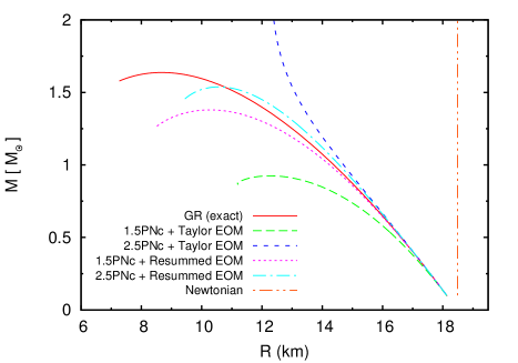
Figure 1: The gravitational mass vs radius (in isotropic coordinates) for static and spherically symmetric stars (described by a perfect fluid obeying a polytropic equation of state with $K=100G^{3}M_{\odot}^{2}/c^{6}$ and $\Gamma=2$), for the various models presented in Sec. VII, for Newtonian theory, and for General Relativity.

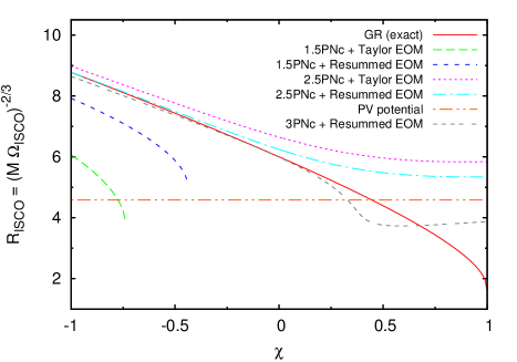
Figure 2: The gauge-invariant ISCO radius $R_{{}_{\rm ISCO}}=(M\Omega_{{}_{ISCO}})^{-2/3}$ of an isolated rotating black hole, for the various models presented in Sec. VII, for the pseudo-Newtonian PV potential, and for General Relativity.

We model isolated stars with a perfect fluid satisfying a polytropic equation of state with $K=100G^{3}M_{\odot}^{2}/c^{6}$ and $\Gamma=2$ (which provides a good approximation for cold neutron stars). Figure 1 shows the gravitational mass $M$ of the stars vs their radius $R$ in isotropic coordinates  for each of the possible models together with the result obtained in full General Relativity. As can be seen the Newtonian prediction for this particular polytropic index is $R=$ const $\approx 18.5$ km independent of the mass. This is clearly very far from the exact general-relativistic result, which is better approximated by our PN schemes, and in particular by the “1.5PNc+resummed EOM” and “2.5PNc+resummed EOM” models.

In the case of black holes, we focus on the ISCO as calculated in each model. The existence of an ISCO has profound astrophysical implications. For instance, the ISCO regulates the radiative efficiency and the location of the inner edge of thin accretion disks, while in compact-object binaries, it marks the boundary where a quasi-adiabatic inspiral transitions into a plunge and merger phase. We thus calculate the gauge-invariant ISCO radius $R_{{}_{\rm ISCO}}=(M\Omega_{{}_{ISCO}})^{-2/3}$, defined in terms of the ISCO orbital frequency $\Omega_{{}_{\rm ISCO}}$. This measure of the ISCO radius is to be preferred to coordinate radii because it does not depend on the coordinate system and is thus free of ambiguities (for instance, while the coordinate location of the ISCO in the PV potential is correct in a particular coordinate system, the associated ISCO frequency is incorrect). To calculate the ISCO frequency we take the Kerr metric in ADM coordinates, as given in sec. VI, truncate it at the appropriate (1.5PN or 2.5PN) order, and utilize it in the Euler equations (with the pressure set to zero), either Taylor expanded at the appropriate (1.5PN or 2.5PN) order, or in their “resummed” form (92). (Of course, the Euler equation reduces to the geodesic equation when $p=0$). The ISCO location is then obtained by studying the stability of circular orbits under radial perturbations. Because circular orbits are assumed to have $\dot{\phi}>0$ (i.e. to move in the positive $\phi$-direction), negative values of the spin-parameter projection $\chi$ denote configurations in which the orbit’s angular momentum and the black-hole spin are anti-aligned.

As can be seen, the “1.5PNc+Taylor EOM” and “1.5PNc+resummed EOM” models do not perform well, because they are far from the general-relativistic result, and for $\chi\gtrsim-0.5$ they do not seem to present an ISCO at all. Better results are achieved by the “2.5PNc+Taylor EOM” and “2.5PNc+resummed EOM” models, which present an ISCO over the whole spin range $\chi\in[-1,1]$. We stress that spin-effects (“frame-dragging”) are completely absent for the PV potential, whose expression $V(r)=-M/(r-2M/c^{2})$ has no spin dependence. Nevertheless, it is rather clear that none of our PN schemes can reproduce the exact general-relativistic result at high spins $\chi\sim 1$. While this behavior is clearly unsatisfactory, it is common to essentially all approximation schemes based on PN theory (even if the PN dynamics is resummed into an EOB model, cf. e.g. Ref. taracchini ). This is because PN theory necessarily fails when $\chi\to 1$, since in the extremal limit the Kerr ISCO coincides with a null generator of the horizon ted_isco , where the PN expansion breaks down as $v\sim c$, i.e. all terms in the PN expansion would be needed to obtain an accurate determination of the ISCO location. In our case, we recall that we are forced by our initial choice of using the Poisson gauge to use the Kerr metric in ADM coordinates, which is only known through 3PN order Hergt:2007ha . (As mentioned earlier, the choice of the Poisson gauge is dictated by the need to minimize the number of propagating degrees of freedom satisfying hyperbolic equations.) The explicit form of the 3PN Kerr metric in ADM coordinates is given by eqs. (66) – (72), and we have attempted to use that form in the unexpanded (“resummed”) geodesic equation $a^{\mu}=0$ to calculate the ISCO. The result is shown in Fig. 2 as “3PNc+resummed EOM”. As can be seen, at high spins that curve still falls short of reproducing the exact Kerr ISCO, confirming that a precise determination of this quantity would require many more PN orders than currently available.

VIII Conclusions

In this work we have presented a PN formulation of the equations of motion for a black hole interacting with a fluid configuration (e.g. a star). Our approach can in principle be implemented in existing Newtonian codes to account for currently missing effects appearing at different PN orders (e.g. frame dragging, black-hole spins, radiation reaction, etc.). Alternatively, it provides for a way to estimate the errors intrinsic to Newtonian approaches because of their neglecting of PN effects. As illustrated in Fig. 1 and 2, our approach is approximate, but its performance improves as higher PN orders are considered (especially for black-hole spin parameters $cJ/(GM^{2})\lesssim 0.5$). Future work will concentrate on the application of this approach in relevant systems.