BENCHMARKING ELECTRON-CLOUD SIMULATIONS AND PRESSURE MEASUREMENTS AT THE LHC

Abstract

During the beam commissioning of the Large Hadron Collider (LHC) [1, 2] with 150, 75, 50 and 25-ns bunch spacing, important electron-cloud effects, like pressure rise, cryogenic heat load, beam instabilities or emittance growth, were observed. A method has been developed to infer different key beam-pipe surface parameters by benchmarking simulations and pressure rise observed in the machine. This method allows us to monitor the scrubbing process (i.e. the reduction of the secondary emission yield as a function of time) in the regions where the vacuum-pressure gauges are located, in order to decide on the most appropriate strategies for machine operation. In this paper we present the methodology and first results from applying this technique to the LHC.

1 Introduction

Since almost 15 years photoemission and secondary emission had been predicted to build up an electron cloud inside the LHC beam pipe [3], similar to the photo-electron instability in positron storage rings [4, 5, 6]. The possibility of “beam-induced multipacting” at the LHC had been suggested even earlier [7] extrapolating from observations with bunched beams at the ISR in the 1970s [8]. The electron cloud, at sufficiently high density, can cause both single and coupled-bunch instabilities of the proton beam [3, 9], give rise to incoherent beam losses or emittance growth [10, 11], heat the vacuum chamber (and subsequently provoke a quench in superconducting magnets), or lead to a vacuum pressure increase by several orders of magnitude due to electron stimulated desorption [12]. All these effects eventually lead to luminosity limitations. Specifically, electron-cloud induced pressure rises have been one of the main performance limitations for some accelerators [11]. From 1999 onward electron-cloud effects have been seen with LHC-type beams first in the SPS, then in the PS, and finally, since 2010, as expected, in the LHC itself. During the early LHC beam commissioning with 150, 75 and 50-ns bunch spacing important electron-cloud effects, such as pressure rise, cryogenic heat load, beam instabilities, beam loss and emittance growth, were observed [13, 14, 15]. Several exploratory studies at the design bunch spacing of 25 ns were performed during 2011 [16].

The LHC mitigation strategy against electron cloud includes a sawtooth pattern on the horizontally outer side of the so-called beam screen inside the cold arcs, a shield mounted on top of the beam-screen pumping slots blocking the direct path of electrons onto the cold bore of the magnets, NEG coating for all the warm sections of the machine, installation of solenoid windings in field-free portions of the interaction region, and, last not least, beam scrubbing, i.e. the reduction of the Secondary Emission Yield (SEY) with increasing electron dose hitting the surface, i.e. as a result of the electron cloud itself. Beam scrubbing represents the ultimate mitigation of electron-cloud effects of the LHC, and it is considered necessary to achieve nominal LHC performance [17].

At injection energy (450 GeV), the pressure inside the vacuum beam pipe affects the speed of the electron-cloud build up, since the initial electrons are produced by gas ionization. However, if there is noticeable multipacting the rate of primary electrons does not significantly influence the final value of the saturated electron density, which is then determined by secondary emission (multipacting) and by the space-charge field of the electron cloud itself. In such case larger vacuum pressures just make the electron density reach its equilibrium value faster. This is due to the fact that the energy spectrum of electrons hitting the wall is insensitive to the pressure [19].

Nevertheless, in order to infer the best estimates of the beam-pipe characteristics, the steady-state vacuum pressure of the machine for each stage of observation has to be introduced as a simulation input parameter, in order to correctly account for the multiturn nature of the pressure evolution in a circular accelerator like the LHC. This is due to the fact that the time constant of the vacuum evolution is much longer than the revolution period, while the electron-cloud build-up simulations typically model only a fraction of a turn. According to the vacuum-gauge measurements, a steady-state pressure is normally established a few minutes after injecting the last bunch train for a given configuration.

Since dedicated in-situ measurements of the LHC electron-cloud density and the LHC vacuum-chamber surface properties are not available we are developing a method to determine the actual surface properties of the vacuum chamber related to secondary emission and to the electron-cloud build up ($\delta_{\textrm{max}}$, $\varepsilon_{\textrm{max}}$ and R [18]; see Fig. 1 for a graphical definition of these three quantities), and their evolution in time, based on benchmarking computer simulations of the electron flux on the chamber surface using the ECLOUD code against pressure measurements for different beam characteristics. This new method allows monitoring the effectiveness of LHC “scrubbing runs” and provides snapshots of the surface conditions around the LHC ring.

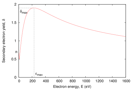
Figure 1: Secondary emission yield for perpendicular incidence as a function of primary electron energy, defining the parameters $\delta_{\textrm{max}}$, $\varepsilon_{\textrm{max}}$ and R.

2 Methodology

The pressure increase due to an electron cloud can be related with the electrons hitting the chamber wall as

$$\Delta P=kT\frac{\int{\eta_{e}(E)\phi_{e}(E)dE}}{S_{eff}}\,,$$ (1)

where $k$ denotes Boltzmann’s constant, $T$ the temperature, $S_{eff}$ the pumping speed, $\eta_{e}$ the electronic desorption coefficient and $\phi_{e}$ the flux of electrons hitting the chamber wall. The quantities $\eta_{e}$ and $S_{eff}$ cannot be introduced in the present electron cloud simulation codes, but assuming that the pressure increase is proportional to the electron flux hitting the chamber wall, pressure measurements for different bunch train configurations (e.g. with changing spacing between trains or with a varying number of trains injected into the machine) can be benchmarked against simulations by comparing ratios of observed pressure increases and of simulated electron fluxes at the wall, respectively. The idea of the benchmarking using ratios goes back to an earlier study for the SPS (serving as LHC injector) where the electron-cloud flux could be measured directly  [20]. In the LHC case, no electron-cloud monitor is available, but instead the measured increase in the vacuum pressure is taken to be a reliable indicator proportional to the electron flux on the wall.

We face a four-parameter problem. The steps followed in the benchmarking are the following:

(1) We fix two of the parameters, namely the pressure (using the measured value) and $\varepsilon_{\textrm{max}}$ (set to 230 eV, which seems to be a good first estimate according to past surface measurements and some previous simulation benchmarking ).

(2) We simulate the electron cloud build up for different bunch configurations using the ECLOUD code, scanning the other two parameters, $\delta_{\textrm{max}}$ and R, in steps of 0.1 and 0.05 respectively. Smaller steps introduce statistical noise which needs to be controlled by smoothing techniques.

(3) For each bunch configuration we plot the simulated electron flux $\phi_{i}$ above a 2D grid spanned by $\delta_{\textrm{max}}$ and R.

(4) We fit the flux simulated on the grid to a third order polynomial and then form the ratio of simulated fluxes (that is, dividing the polynomials) for two different bunch configurations [the fluxes and not their ratio are fitted in order to suppress the effect of statistical fluctuations].

(5) Comparing the latter ratio with the experimental ratio of measured pressure increases yields a curve in the $\delta_{\textrm{max}}$-R plane (see Fig. 2). Different configurations yield different curves in that plane.

(6) If the measurements contain sufficient information and the simulation model is reasonably accurate we expect to obtain a unique intersection between lines corresponding to different bunch configurations. This crossing point then defines the solution for $\delta_{\textrm{max}}$ and R.

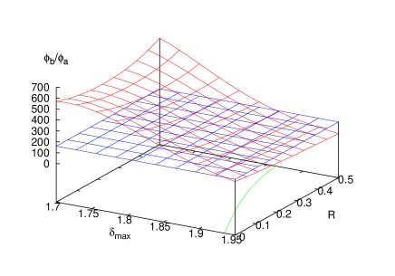
Figure 2: Example of a 3D surface of simulated fluxes for the case $\phi_{b}/\phi_{a}$ (red) cut by a plane surface (blue) at the value equal to the ratio of the corresponding measured pressures ($P_{b}/P_{a}=161.0$). The bottom plane shows the contour of the intersection between both surfaces (green).

We apply this methodology for certain LHC regions in which pressure gauges and vacuum pumps are located. Normally these are installed in short beam-pipe modules made from copper-coated stainless steel mounted between two NEG coated pipes (7 m long each), with a good pumping and (after activation) low secondary emission yield, so that we may assume that the pressure rise measured at a gauge is the result of the electron cloud produced exclusively within the gauge’s vacuum module. The module vacuum chamber is round with 80 mm diameter. In the following we only present results for one ionization gauge. Results for other gauges look similar.

3 Results

Until now we have processed 4 sets of measurements obtained during the conditioning of the machine through beam scrubbing. All of these have been recorded at a beam energy of 450 GeV with either 50-ns or 25-ns bunch spacing for the first 3 sets and the last set, respectively.

We have used two kinds of beam configurations, with varying spacing between successive bunch trains (also called “batches”) and varying number of batches, respectively. Table 1 lists the parameters for the three sets of measurements with 50 ns bunch spacing.

Table 1: Parameters used in the simulations for the different sets of measurements with 50 ns bunch spacing. In sets 2 and 3 there is an additional space of 225 ns between the two (set 2) or three trains (set 3) of 36 bunches injected simultaneously.

	Set 1	Set 2	Set 3
# of bunches	36	72 (2x36)	108 (3x36)
per batch
# of batches	1 - 5	1 - 14	1 - 12
Batch spacing	2.0 - 6.0	4.850	0.925
($\mu$s)
Av. bunch	1.1	1.21	1.15
population
($10^{11}$ ppb)

At the beginning of a scrubbing run in April 2011, two experiments were carried out (both corresponding to set 1 listed above). In the first we injected batches in pairs with varying batch spacing (6 $\mu$s, 4 $\mu$s and 2 $\mu$s). Each pair of batches was separated by 11.5 $\mu$s (a time considered long enough to clear any electron cloud). Figure 3 shows the pressure increases observed during this first experiment, including an additional first, shorter 12-bunch batch introduced for machine-protection reasons (and where no pressure increase can be appreciated). In the second experiment we injected an increasing number of batches at a batch-to-batch distance of 2.125 $\mu$s (up to 5).

Figure 4 depicts the results obtained for both experiments. We could conclude that the solution is around $\delta_{\textrm{max}}=1.9$ and $R=0.2$. We have to take into account that there are large uncertainties in the measured pressure values as well as in the estimated bunch population. According to simulations, such uncertainties can lead to a mismatch between lines and prevent a single unique intersection, as seen for this example. The value of $\delta_{\textrm{max}}=1.9$ is in agreement with an estimate from the CERN vacuum group, which expected an initial value between 1.6 and 1.9 [22, 23]. In addition, the value $R=0.2$ is in agreement with several high precision measurements, both recent (e.g. [24]) and old (e.g. [25]).

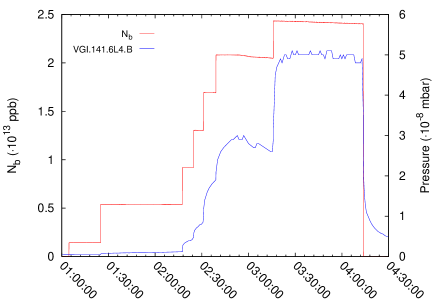
Figure 3: Beam intensity and pressure at the gauge VGI.141.6L4.B during the first experiment on 6 April 2011. Every step in the beam intensity (red curve) indicates the injection of a new batch.

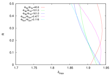
Figure 4: Combinations of $\delta_{\textrm{max}}$-R values characterizing the chamber surface, obtained by benchmarking ratios of observed pressure increases against ratios of simulated electron fluxes, for measurements on 6 April 2011.

After a few days of surface conditioning, double batches of 36 bunches each separated by 225 ns were injected at a distance of 4.85 $\mu$s (up to 14). This corresponds to the set 2 of experimental data. A similar experiment (set 3) took place in mid May 2011 but using triple batches instead, again separated by 225 ns, at a distance of 925 ns (up to 12). Figure 5 shows the results obtained in these cases. It is worth noting that for these last two cases we observe parallel lines instead of a clear intersection between the lines. This is due to the loss of sensitivity to the effect of the 225 ns gap between 36-bunch batches, that appears when the double (or triple) batches are injected together instead of one after the other. Indeed the lines should be identical under some plausible simplifying assumptions. The conclusion is that it is necessary, during the same experiment, to take two sets of measurements with different batch spacings, in order to obtain lines of different slope which uniquely intersect and yield the desired parameter information.

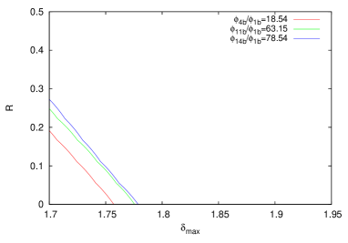
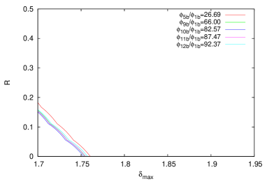
Figure 5: Combinations of $\delta_{\textrm{max}}$-R values characterizing the chamber surface, obtained by benchmarking ratios of observed pressure increases against ratios of simulated electron fluxes, for LHC measurements taken on 11 April (top) and 19 May 2011 (bottom).

A new measurement, with varying spacing between batches, has been carried out at the end of the 2011’s proton run (end October). On this occasion the bunch spacing was reduced to 25 ns. Table 2 shows the parameters used in this case and Fig. 6 depicts the result obtained for this experiment.

Table 2: Parameters used in the simulations for the measurements with 25 ns bunch spacing.

	Set 4
# of bunches	72
per batch
# of batches	2
batch spacing ($\mu$s)	1.0, 2.0, 3.0, 4.0
bunch population	1.1, 1.0, 1.0, 1.1
($10^{11}$ ppb)

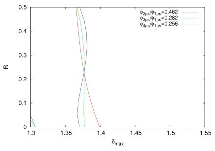
Figure 6: Combinations of $\delta_{\textrm{max}}$-R values characterizing the chamber surface, obtained by benchmarking ratios of observed pressure increases against ratios of simulated electron fluxes, for LHC measurements taken on 25 October 2011. In this case a value $\varepsilon_{\textrm{max}}=260$ eV has been assumed, as it gives a better fit to the data. This could be a sign of variation of $\varepsilon_{\textrm{max}}$ during the scrubbing.

Although we are not yet able to extract a unique value for $\delta_{\textrm{max}}$ and R, we can clearly see evidence for conditioning, as the solution for later cases tends towards lower $\delta_{\textrm{max}}$ values. Figure 7 summarizes the approximate time evolution of $\delta_{\textrm{max}}$ in the “warm-warm” transition regions where pressure gauges are located.

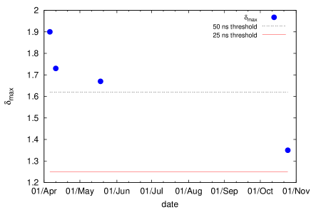
Figure 7: Approximate time evolution (from April to October 2011) of $\delta_{\textrm{max}}$ in the uncoated warm straight sections (chamber radius 40 mm). The lowest values reachable with scrubbing corresponds to the 25-ns multipacting threshold, for a reflectivity $R$ of 0.2. The first injection of a beam with 25-ns bunch spacing beam took place on 29 June 2011.

We can see that the evolution of the conditioning for 50-ns and 25-ns beams looks as expected, with $\delta_{\rm max}$ approaching the simulated multipacting thresholds for 50-ns or 25-ns bunch spacing (both also indicated in the figure), respectively, as asymptotic limit. All these facts instill some confidence in the method and support its potential use as a tool for monitoring the surface conditioning through beam scrubbing.

The evolution in the uncoated straight sections goes from an initial value of $\delta_{\textrm{max}}\approx 1.9$ at the beginning of the scrubbing run in April 2011 to $\delta_{\textrm{max}}\approx 1.35$ when the experiments with 25 ns were carried out. The points shown for 11 April and 19 May 2011 have been obtained by assuming the value of an average line in Fig. 5 at $R=0.2$.

4 Conclusions

In 2010 and 2011 first electron-cloud effects have been observed with proton beams in the LHC. Rapid surface conditioning has allowed reducing the bunch spacing for nominal operation from 150 ns over 75 ns down to 50 ns without any significant perturbation from electron cloud.

Thanks to the benchmarking of vacuum observations against simulations described in this paper, we have been able to monitor the evolution of $\delta_{\textrm{max}}$ during machine conditioning in the warm straight sections of the LHC. The observable considered is the pressure increase resulting from the electron cloud, which is taken to be proportional to the electron flux impinging on the vacuum chamber walls. Namely, by benchmarking the ratios of experimental pressures and of simulated electron fluxes for different beam configurations (e.g., for varying spacing between bunch trains or varying number of batches) we can then pin down the value of the maximum secondary emission yield as well as the reflection probability for low-energy electrons. Applying this method to each of the different measurement sets available so far provides clear evidence for surface conditioning in the uncoated warm regions of the LHC, from an initial maximum secondary emission yield of about 1.9 down to about 1.35, with $R\approx 0.2$, as can be seen in Fig. 7.

In order to reach the design LHC bunch spacing of 25 ns in physics operation, further conditioning of the secondary emission yield is still required. According to some estimates [26], approximately 2 weeks of machine time would be required to achieve these values, since the scrubbing effect reduces with decreasing $\delta_{\textrm{max}}$.

5 Acknowledgements

The authors would like to thank G. Arduini, V. Baglin, G. Bregliozzi, G. Iadarola, G. Lanza, E. Métral, G. Rumolo, M. Taborelli and C. Yin-Vallgren for relevant and always enriching discussions and experimental data as well as all the machine operators for the support they provided with the machine operation during the experiments.

References

- [1] O. Brüning et al (eds.), LHC Design Report, v. 1, CERN-2004-003 (2004).
- [2] O. Brüning, H. Burkhart and S.Myers, ”The Large Hadron Collider”, Progress in Particle and Nuclear Physics, Volume 67, Issue 3, July 2012, Pages 705-734.
- [3] F. Zimmermann, “A Simulation Study of Electron-Cloud Instability and Beam-Induced Multipacting in the LHC”, LHC Project-Report 95 (1997).
- [4] M. Izawa et al., Phys. Rev. Lett., Vol. 74 No. 8 (1995).
- [5] K. Ohmi, Phys. Rev. Lett. 75: 1526-1529 (29915).
- [6] M.A. Furman, G.R. Lambertson, Proc. EPAC’06, p. 1087 (1996).
- [7] O. Gröbner, Vacuum 47, 591 (1996).
- [8] O. Gröbner, 10th Int. Conference on High Energy Accelerators, Protvino (1977).
- [9] F. Zimmermann, “Review of single bunch instabilities driven by an electron cloud”, PRST-AB 7, 124801 (2004).
- [10] E. Benedetto, G. Franchetti and F. Zimmermann, ”Incoherent effects of electron clouds in proton storage rings”, Phys.Rev.Lett.97:034801, 2006.
- [11] W. Fischer et al., ”Electron cloud observations and cures in the Relativistic Heavy Ion Collider”, Phys. Rev. ST Accel. Beams 11, 041002 (2008).
- [12] J.M. Jimenez et al., Proc. ECLOUD’02, CERN, Geneva, CERN-2002-001 pp. 17 (2002).
- [13] J.M. Jimenez et al., “First observations 50 and 75 ns operation in the LHC: Vacuum and Cryogenics observations”, ATS/Note/2011/NNN (MD), 2011. Proc. Chamonix 2011 LHC Performance Workshop, CERN-2011-005 pp. 63 (2011).
- [14] G. Arduini et al., “First observations 50 and 75 ns operation in the LHC: Vacuum and Cryogenics observations”, Proc. Chamonix 2011 LHC Performance Workshop, CERN-2011-005 pp. 56 (2011).
- [15] G. Rumolo et al., ”Electron cloud observation in the LHC”, Proc. IPAC’11, San Sebastian pp.2862 (2011).
- [16] G. Rumolo et al., ”Electron cloud effects in the LHC in 2011”, Proc. LHC Beam Operation Workshop’11, Evian (2011).
- [17] O. Brüning et al., “Electron Cloud and Beam Scrubbing in the LHC”, Proc. PAC’99, New York pp. 2629 (1999).
- [18] R. Cimino et al., Phys. Rev. Lett. 93:014801 (2004).
- [19] U. Iriso “Electron Clouds Thresholds with 75 ns Bunch Spacing”, EuCARD-AccNet document, to be published.
- [20] D. Schulte et al., “Electron cloud measurements in the SPS in 2004”, Proc. PAC’05 Knoxville pp.1371 (2005).
- [21] C. Yin Vallgren, ”Low Secondary Electron Yield Carbon Coatings for Electron Cloud Mitigation in Modern Particle Accelerators”, PhD thesis,CERN-THESIS-2011-063 (2011).
- [22] N. Hilleret et al., LHC Project Report 433 2000, EPAC 00.
- [23] C. Scheuerlein et al., Appl.Surf.Sci 172(2001).
- [24] M. Belhaj, ”ONERA/CNES simulation models and measurements for SEY”, elsewhere these proceedings.
- [25] I. Kaganovich, ”Secondary Electron Emission in the Limit of Low Energy and its Effect on High Energy Physics Accelerators”, elsewhere these proceedings.
- [26] G. Rumolo et al., ”LHC experience with different bunch spacings in 2011 (25, 50 and 75ns)”, Proc. Chamonix 2012 LHC Performance Workshop, to be published.