Quantum Fluctuation Relations for Ensembles of Wave Functions

Abstract

New quantum fluctuation relations are presented. In contrast with the the standard approach, where the initial state of the driven system is described by the (micro)canonical density matrix, here we assume that it is described by a (micro)canonical distribution of wave functions, as originally proposed by Schrödinger. While the standard fluctuation relations are based on von Neumann measurement postulate, these new fluctuation relations do not involve any quantum collapse, but involve instead a notion of work as the change in expectation of the Hamiltonian.

1 Introduction

In the last two decades the field of non-equilibrium thermodynamics has undergone a tremendous advancement due to the discovery of exact non-equilibrium relations (named fluctuation relations) which characterize non-equilibrium processes well beyond the regime of linear response, and provide a deep insight into statistical nature and microscopic origin of the second law of thermodynamics. The most prominent example of such exact relations is the Jarzynski equality [1] which allows for obtaining the free energy landscape of small systems, like a single DNA molecule, from very many measurements of work done on the system as it is driven out of equilibrium, e.g., by stretching the molecule [2]. A related result, known as Crooks work fluctuation theorem [3], relates the free energy to the probability of performing work $W$ during the process and the probability of performing work $-W$ during the time-reversed process. These results, which have been first obtained within the framework of classical mechanics were later derived also within the quantum mechanical framework [4, 5, 6, 7].

The crucial ingredient needed for obtaining the fluctuation relations in the quantum case is the so called two measurements scheme [8, 9]. In this scheme the system energy is measured at the beginning and end of the driving protocol and the work is defined as the difference of the outcomes of these measurements:

$$W=E_{m}^{\tau}-E_{n}^{0}$$ (1)

where $E_{k}^{t}$ denotes an eigenvalue of the (time-dependent) Hamilton operator $\hat{H}(\lambda_{t})$ at time $t$. As usual, here it is assumed the Hamilton operator changes in time due to the time dependence of an external parameter $\lambda_{t}$. This scheme relies on the von Neumann measurement postulate according to which the measurement process induces the collapse of the wave function on one of the eigenstates of the measured observable, i.e, $\hat{H}(\lambda_{0})$ and $\hat{H}(\lambda_{\tau})$ in the present case. Notably, experimental verification and application of the quantum fluctuation relations based on the two-measurement scheme have not been accomplished yet, while alternative strategies aimed at avoiding the two projective measurements have been proposed. Two prominent examples propose to replace them with many weak measurements during the driving protocol [10], or with state tomography of one or two qubit ancillae appropriately coupled to the driven system [11, 12, 13, 14]

With this work we establish new quantum fluctuation relations, which look exactly like the standard quantum fluctuation relations but substantially differ from them due to a different underlying definition of quantum work, and a different ensemble specifying the initial condition. As in the standard case [8, 9] we assume an initial statistical ensemble, but at variance with the ordinary quantum statistical mechanics, we assume that the statistical ensemble is described by a distribution of wave functions as originally suggested by Schrödinger [15], later pursued by Khinchin [16] and recently advocated by an increasing number of authors [17, 18, 19, 20, 21, 22, 23, 24, 25, 26, 27, 28, 29]. We will establish fluctuation relations for the microcanonical [19, 23, 26, 25, 27, 28] and canonical [17, 30] wave function ensembles. Most remarkably these new fluctuation relations naturally involve a notion of work as the change in the expectation of the Hamiltonian operator

$$w=\langle\psi(\tau)|\hat{H}(\lambda_{\tau})|\psi(\tau)\rangle-\langle\psi(0)|\hat{H}(\lambda_{0})|\psi(0)\rangle\,.$$ (2)

Accordingly they do not involve von Neumann measurement postulate. In Eq. (2) $|\psi(0)\rangle$ is a wave function randomly chosen from the distribution, and $|\psi(\tau)\rangle$ is its time evolution. Just as with the classical fluctuation theorems, the stochastic nature of $w$ comes from the fact that the initial state $|\psi(0)\rangle$ is randomly drawn from a distribution, while its evolution is deterministic.

So, the interpretation framework that is adopted here is that experimentally observed quantities correspond to their quantum mechanical expectation, an approach that is at least as common in the scientific literature and effective as that involving wave function collapses. To give one example, Kubo’s linear response theory [31], is a theory of quantum expectations which mentions no collapses. This same philosophy has been advocated by G. Jona-Lasinio and C. Presilla [30], who pointed out that the wave function ensembles could be good candidates for the study of mesoscopic systems, where robust coherence phenomena are involved.

2 Wave function ensembles

We consider a quantum system with a finite dimensional Hilbert space of dimension $N$. Each wave function $|\psi\rangle$ can be represented by an $N$ dimensional complex vector $\mathbf{c}$, and the system Hamilton operator $\hat{H}(\lambda)$ can be represented by a $N\times N$ Hermitean matrix $\mathbf{H}(\lambda)$. Following Ref. [32] we introduce the suggestive notation

$$\mathbf{c}=\mathbf{x}+i\mathbf{p}$$ (3)

$$h(\mathbf{x},\mathbf{p};\lambda_{t})=(\mathbf{x}-i\mathbf{p})^{T}\mathbf{H}(\lambda_{t})(\mathbf{x}+i\mathbf{p})$$ (4)

where $\mathbf{x}$ and $\mathbf{p}$ are the real and imaginary parts of $\mathbf{c}$, $h(\mathbf{x},\mathbf{p},\lambda_{t})$ denotes the expectation of the Hamilton operator on the state $\mathbf{x}+i\mathbf{p}$, $\mathbf{z}^{T}$ denotes transpose of $\mathbf{z}$, and matrix multiplication is implied. We stress that $\mathbf{x}$ and $\mathbf{p}$ should not be confused with positions and momenta.

Below we shall consider statistical ensembles $\rho(\mathbf{x},\mathbf{p})$ defined on the wave function “phase space” $(\mathbf{x},\mathbf{p})$. Given an observable $\hat{B}$, with matrix representation $\mathbf{B}$, its ensemble average is its wave function expectation $b(\mathbf{x},\mathbf{p})=(\mathbf{x}-i\mathbf{p})^{T}\mathbf{B}(\mathbf{x}+i\mathbf{p})$, averaged over the wave function distribution, namely

$$\langle\hat{B}\rangle=\int d\mathbf{x}d\mathbf{p}\,\rho(\mathbf{x},\mathbf{p})b(\mathbf{x},\mathbf{p})\,.$$ (5)

2.1 Microcanonical wave function ensemble

In the microcanonical wave function ensemble [19, 23, 26, 25, 27, 28] all wave functions $(\mathbf{x},\mathbf{p})$ with a given expectation of energy $E=h(\mathbf{x},\mathbf{p};\lambda)$ have same probability, whereas all other wave functions have probability zero. For a fixed $\lambda$ it reads:

$$\rho_{\mu}(\mathbf{x},\mathbf{p};E,\lambda)=\frac{\delta(E-h(\mathbf{x},\mathbf{p};\lambda))\delta(1-|\mathbf{x}+i\mathbf{p}|^{2})}{\Omega(E,\lambda)}$$ (6)

where $\delta$ denotes Dirac’s delta function, and

$$\Omega(E,\lambda)=\int d\mathbf{x}d\mathbf{p}\,\delta(E-h(\mathbf{x},\mathbf{p};\lambda))\delta(1-|\mathbf{x}+i\mathbf{p}|^{2})$$ (7)

is the density of states. Note the formal similarity with the classical microcanonical ensemble. The main the difference is the presence of the extra factor $\delta(1-|\mathbf{x}+i\mathbf{p}|^{2})$ which restricts the integration to the “physical Hilbert space”, namely the subspace of normalized wave functions, also known as the projective Hilbert space. Note that at variance with the textbook quantum microcanonical ensemble [33, 34], in which only those eigenstates of the Hamiltonian in a narrow interval around the energy $E$ contribute, here all eigenstates participate to the ensemble. For this reason various authors claim that the ensemble in Eq. (7) provides a more realistic description of the thermodynamics of isolated systems [25, 26, 27, 28]. Another pleasing property of this ensemble is that, at variance with the standard microcanonical ensemble, it does not require a dense energy spectrum, and can therefore be well applied to small quantum systems with well separated energy levels. Indeed, the ensemble depends continuously on the real parameters $E,\lambda$, which makes the derivation of the associated thermodynamics straightforward also in case of small systems [24]. Ref. [28] shows that this ensemble well describes the statistics of a small thermally isolated system after repeated non-adiabatic perturbations.

2.2 Canonical wave function ensemble

In the canonical wave function ensemble [17, 30], wave functions are weighted with the Gibbs factor $e^{-\beta h(\mathbf{x},\mathbf{p};\lambda)}$:

$$\rho_{c}(\mathbf{x},\mathbf{p};\beta,\lambda)=\frac{e^{-\beta h(\mathbf{x},\mathbf{p};\lambda)}\delta(1-|\mathbf{x}+i\mathbf{p}|^{2})}{Z(\beta,\lambda)}$$ (8)

where

$$Z(\beta,\lambda)=\int d\mathbf{x}d\mathbf{p}\,e^{-\beta h(\mathbf{x},\mathbf{p};\lambda)}\delta(1-|\mathbf{x}+i\mathbf{p}|^{2})$$ (9)

Note again the formal similarity with the classical canonical ensemble. In Ref. [30] this ensemble is called the Schrödinger-Gibbs ensemble. According to [18] this ensemble can give realistic predictions in case of mesoscopic systems where robust coherence phenomena are involved.

3 Rationale for wave function ensembles

A criterion for establishing the goodness of a statistical ensembles as a candidate model of equilibrium thermodynamics is whether the ensemble is invariant under the time evolution. As will become clearer in the next section this is indeed the case for the canonical and microcanonical wave function ensemble.

Another criterion, which traces back to Boltzmann [35], is whether the ensemble endows the parameter space with a “thermodynamic structure”. To be more explicit, given a statistical ensemble $\rho(\Gamma,X_{i})$, (defined on a phase space $\Gamma$ and on a parameter space $X_{i}$), one checks whether there exist an integrating factor $\gamma(X_{i})$, such that

$$\gamma\,\delta Q=\quad exactdifferential$$ (10)

where $\delta Q$ is the heat differential as calculated in the ensemble. This equation is known as the heat theorem, and is the most fundamental equation of thermodynamics. Prominent examples of textbooks that take this viewpoint in establishing the foundations of quantum statistics are those of Schrödingier [15], and Khinchin [16].

To calculate $\delta Q$ use the standard formula

$$\delta Q=dE+Fd\lambda$$ (11)

where

$$E=\langle\hat{H}\rangle$$ (12)

$$F=-\left\langle\frac{\partial\hat{H}}{\partial\lambda}\right\rangle$$ (13)

denote the ensemble averages of energy and of the generalized force conjugated to the external parameter. Note that in case of a single parameter $\lambda$, mathematics ensures that an integrating factor always exists. A differential form in two dimensions (i.e., $E$ and $\lambda$, in Eq. (11)), always admits an integrating factor. However, the system Hamiltonian may depend on many external parameters $\lambda_{i}$, hence $\delta Q=dE+\sum_{i}F_{i}d\lambda_{i}$, which makes the question of the existence of an integrating factor non-trivial.

3.1 Canonical case

In the canonical case we have

$$E=E(\beta,\lambda)=\int d\mathbf{x}d\mathbf{p}\,\rho_{c}(\mathbf{x},\mathbf{p};\beta,\lambda)h(\mathbf{x},\mathbf{p};\lambda)$$ (14)

$$F=F(\beta,\lambda)=-\int d\mathbf{x}d\mathbf{p}\,\rho_{c}(\mathbf{x},\mathbf{p};\beta,\lambda)\frac{\partial h(\mathbf{x},\mathbf{p};\lambda)}{\partial\lambda}$$ (15)

In this case $\beta$ is an integrating factor for $\delta Q$ and $S_{c}(\beta,\lambda)=\beta E(\beta,\lambda)+\ln Z(\beta,\lambda)$ is the associated generating function. The argument follows step by step the classical derivation [36], which can be repeated without modifications. The partial derivatives of $S_{c}(\beta,\lambda)$ are:

$$\frac{\partial S_{c}}{\partial\beta}=E+\beta\frac{\partial E}{\partial\beta}+\frac{1}{Z}\frac{\partial Z}{\partial\beta}=\beta\frac{\partial E}{\partial\beta}$$ (16)

$$\frac{\partial S_{c}}{\partial\lambda}=\beta\frac{\partial E}{\partial\lambda}+\frac{1}{Z}\frac{\partial Z}{\partial\lambda}=\beta\frac{\partial E}{\partial\lambda}+\beta F$$ (17)

therefore

$$dS_{c}=\beta\left(\frac{\partial E}{\partial\beta}d\beta+\frac{\partial E}{\partial\lambda}d\lambda+Fd\lambda\right)=\beta(dE+Fd\lambda)=\beta\delta Q$$ (18)

The derivation can be straightforwardly repeated in the case of many parameters. We remark that there are however infinitely many integrating factors for $\delta Q$. So having found one does not ensure by itself that it can be interpreted as inverse temperature, and that the associated generator of the exact differential can be interpreted as entropy. Take for example $g(\beta,\lambda)=f(S_{c}(\beta,\lambda))$ with any monotonic function $f$. Then $dg=f^{\prime}(S_{c}(\beta,\lambda))dS_{C}=f^{\prime}(S_{c}(\beta,\lambda))\beta\delta Q$, where $f^{\prime}$ is the derivative of $f$. This says that $f^{\prime}(S_{c}(\beta,\lambda))\beta$, is also an integrating factor for $\delta Q$. In order to pick the “thermodynamic” integrating factor, we need an extra ingredient. We thus further require that the entropy be additive. Namely, if two non interacting and non-entangled systems have separately the entropies $S_{1}$ and $S_{2}$, the entropy of the total system should be $S_{1}+S_{2}$. The requirement of non-entanglement is very crucial here. It restricts the Hilbert space of the compound system, from a tensor product of dimension $N_{1}N_{2}$ to the direct product of dimension $N_{1}+N_{2}$. In this “classical” phase space the canonical wave function distribution of the compound system reduces to the product of the canonical wave function distributions for each subsystem, so does the partition function $Z$. Noting that the energy is additive, it follows that $S_{c}(\beta,\lambda)$ is additive as well, which singles it out as a good candidate for thermodynamic entropy. Accordingly $\beta$ is the inverse temperature.

3.2 Microcanonical case

In the microcanonical case

$$E=\int d\mathbf{x}d\mathbf{p}\,\rho_{\mu}(\mathbf{x},\mathbf{p};E,\lambda)h(\mathbf{x},\mathbf{p};\lambda)$$ (19)

$$F=F(E,\lambda)=-\int d\mathbf{x}d\mathbf{p}\,\rho_{\mu}(\mathbf{x},\mathbf{p};E,\lambda)\frac{\partial h(\mathbf{x},\mathbf{p};\lambda)}{\partial\lambda}$$ (20)

An integrating factor for $\delta Q$ is in this case the function $\Omega(E,\lambda)/\Phi(E,\lambda)$, where, in analogy with classical mechanics

$$\Phi(E,\lambda)=\int d\mathbf{x}d\mathbf{p}\,\theta(E-h(\mathbf{x},\mathbf{p};\lambda))\delta(1-|\mathbf{x}+i\mathbf{p}|^{2})$$ (21)

denotes the volume of physical Hilbert space with energy expectation below $E$. As in classical mechanics, we have $\Phi(E,\lambda)=\int_{E_{0}}^{E}\Omega(E^{\prime},\lambda)dE^{\prime}$, where $E_{0}$ is the ground state energy. The symbol $\theta$ denotes the Heaviside step function. The proof follows, mutatis mutandis, the classical argument (the generalized Helmholtz theorem) [37], which can be repeated also with many external parameters. The generating function associated with the integrating factor $\Omega/\Phi$ is $S_{\mu}(E,\lambda)=\ln\Phi(E,\lambda)$. In this case the requirement of additivity does not seem to single $S_{\mu}(E,\lambda)$ so straightforwardly as in the canonical case. The reason is that, unlike the exponential, the theta function does not factorize in the product of two theta functions. Classically this problem can be easily circumvented upon noticing that the integrating factor $\Omega/\Phi$ equals the average kinetic energy per degree of freedom (equipartition theorem [38]), which singles it out as the thermodynamic temperature. In quantum mechanics however there is no equipartition theorem to help us. We leave the resolution of this question to future studies.

It should be remarked that our present analysis contrasts with Ref. [24], where thermodynamics was derived from the logarithm of the density of states, namely $\ln\Omega(E,\lambda)$. We remark that this choice does not comply with the heat theorem, Eq. (24), namely, there does not exist, in general a function $\gamma(E,\lambda)$, such that $\gamma(E,\lambda)\delta Q$ would equal the differential of $\,\ln\Omega(E,\lambda)$. This very same question appears also at the classical level, where it has been long ignored due to the fact that in most cases of interest the “surface entropy” (logarithm of the density of states) and the “volume entropy” (logarithm of the integrated density of states), give practically undistinguishable results for sufficiently large systems [37, 39].

4 Fluctuation relations

Fluctuation relations for the wave function ensembles follow straightforwardly upon noticing that in the $(\mathbf{x},\mathbf{p})$ representation, the Schrödinger equation

$$i\hbar\dot{\mathbf{c}}=\mathbf{H}(\lambda_{t})\mathbf{c}$$ (22)

assumes the form of classical Hamilton’s equation

$$\dot{\mathbf{x}}=\frac{\partial}{\partial\mathbf{p}}h(\mathbf{x},\mathbf{p};\lambda_{t})$$ (23)

$$\dot{\mathbf{p}}=-\frac{\partial}{\partial\mathbf{x}}h(\mathbf{x},\mathbf{p};\lambda_{t})$$ (24)

with the function $h(\mathbf{x},\mathbf{p};\lambda_{t})$ being the generator of the dynamics [32]. In analogy with the classical case, we introduce the following notion of quantum work

$$w=h(\mathbf{x}_{\tau},\mathbf{p}_{\tau};\lambda_{\tau})-h(\mathbf{x},\mathbf{p};\lambda_{0})$$ (25)

where $(\mathbf{x}_{\tau},\mathbf{p}_{\tau})$ denotes the evolved of $(\mathbf{x},\mathbf{p})$, according to Hamilton’s equations (24). Physically, $w$ is the change in the expectation of the Hamilton operator $\hat{H}$, due to the evolution of the wave function $|\psi\rangle$, see Eq. (2). Note that $w$ can be expressed as an integrated power:

$$w=\int_{0}^{\tau}dt\dot{\lambda}_{t}\frac{\partial h(\mathbf{x}_{t},\mathbf{p}_{t},\lambda_{t})}{\partial\lambda_{t}}$$ (26)

In equilibrium, namely for a constant $\lambda$, energy conservation and Liouville theorem ensure that surfaces of constant energy expectation in the physical Hilbert space will be mapped onto themselves by the time evolution, implying that, as anticipated, the canonical and microcanonical wave function ensembles are stationary [18].

The probability that the work $w$ be performed on a system prepared in a wave function ensemble $\rho(\mathbf{x},\mathbf{p})$ can be written as

$$p(w)=\int d\mathbf{x}d\mathbf{p}\,\rho(\mathbf{x},\mathbf{p})\delta(w-h(\mathbf{x}_{\tau},\mathbf{p}_{\tau},\lambda_{\tau})+h(\mathbf{x},\mathbf{p},\lambda_{0}))$$ (27)

Noticing that the evolution (24) conserves the normalization, ${|\mathbf{x}_{\tau}+i\mathbf{p}_{\tau}|^{2}=|\mathbf{x}+i\mathbf{p}|^{2}=1}$ (unitarity of quantum evolution) and is volume preserving, $d\mathbf{x}_{\tau}d\mathbf{p}_{\tau}=d\mathbf{x}d\mathbf{p}$ (classical Liouville theorem), one can repeat step by step the derivations of classical microcanonical [40] and canonical [2] fluctuation relations, upon requiring that the Hamilton operator is time reversal invariant.

In the microcanonical case one obtains:

$$\frac{p_{E}(w)}{\widetilde{p}_{E+w}(-w)}=\frac{\Omega(E+w,\lambda_{\tau})}{\Omega(E,\lambda_{0})}$$ (28)

where $p_{E}(w)$ is the probability of doing work $w$ when the initial state is randomly drawn from the distribution $\rho_{\mu}(\mathbf{x},\mathbf{p};E,\lambda_{0})$ under the driving protocol $\lambda_{t}$ $t\in[0,\tau]$ , and $\widetilde{p}_{E+w}(-w)$ is the probability of doing work $-w$ when the initial state is randomly drawn from ${\rho_{\mu}(\mathbf{x},\mathbf{p};E+w,\lambda_{\tau})}$ under the protocol $\lambda_{\tau-t}$, $t\in[0,\tau]$.

In the canonical case one obtains:

$$\frac{p(w)}{\widetilde{p}(-w)}=\frac{Z(\beta,\lambda_{\tau})}{Z(\beta,\lambda_{0})}e^{\beta w}=e^{-\beta(\Delta F-w)}$$ (29)

where $p(w)$ is the probability of doing work $w$ when the initial state is randomly drawn from the distribution $\rho_{c}(\mathbf{x},\mathbf{p};\beta,\lambda_{0})$ under the driving protocol $\lambda_{t}$ $t\in[0,\tau]$ , and $\widetilde{p}(-w)$ is the probability of doing work $-w$ when the initial state is randomly drawn from ${\rho_{c}(\mathbf{x},\mathbf{p};\beta,\lambda_{\tau})}$ under the protocol $\lambda_{\tau-t}$, $t\in[0,\tau]$. In analogy with the classical case we have introduced the notation $\Delta F=F(\beta,\lambda_{\tau})-F(\beta,\lambda_{0})$, with $F(\beta,\lambda)=-\beta^{-1}\ln Z(\beta,\lambda)$. We stress that this free energy $F(\beta,\lambda)$ may considerably differ from the usual free energy $F_{st}(\beta,\lambda)=-\beta^{-1}\ln\mbox{Tr}e^{-\beta\hat{H}(\lambda)}$, see Fig. 1.a.

5 Illustrative example

To better clarify the differences and similarities between the standard quantum fluctuation relations and the quantum fluctuation relations for wave function ensembles, we consider the Landau-Zener(-Stückelberg-Majorana) [42, 43, 44, 45] problem

$$\hat{H}(\lambda_{t})=\lambda_{t}\sigma_{z}+\Delta\sigma_{x}\,,\qquad\lambda_{t}=vt/2\,.$$ (30)

It governs the dynamics of a two-level quantum system whose energy separation, $vt$, varies linearly in time, and whose states are coupled via the interaction energy $\Delta$. For example, a spin-$1/2$ particle with magnetic moment $\mu$ in a magnetic field $\vec{B}_{t}=-(\Delta/\mu,0,vt/2\mu)$. Here, $\sigma_{x}$ and $\sigma_{z}$ denote Pauli matrices.

Let us assume the two-level system is in a state described by the canonical wave function ensemble, Eq. (8). Let $\mathbf{c}=(a,b)^{T}$, with $a,b\in\mathbb{C}$, denote a point in the Hilbert space (a wave function). The energy expectation $h(a,b,\lambda)$ over the state $\mathbf{c}$ reads $h(a,b;\lambda)=\lambda(|a|^{2}-|b|^{2})+\Delta(a^{*}b+ab^{*})$, where ^∗ denotes complex conjugation. Accordingly, the partition function reads:

$$Z(\beta,\lambda)=\int da\,db\,e^{-\beta[\lambda(|a|^{2}-|b|^{2})+\Delta(a^{*}b+ab^{*})]}\delta(1-|a|^{2}-|b|^{2})$$ (31)

As is well known, the projective Hilbert space of a two-level system can be mapped onto a sphere of unit radius in $\mathbb{R}^{3}$, the Bloch sphere. Accordingly, the partition function $Z(\beta,\lambda)$ can be expressed as an integral over the Bloch sphere. This is accomplished by the following change of variables, $a=e^{i\phi}r\cos\gamma/2,b=e^{i\phi}re^{i\delta}\sin\gamma/2$, where $r\in[0,\infty),\phi\in[0,2\pi],\gamma\in[0,\pi],\delta\in[0,2\pi]$, leading to:

$$Z(\beta,\lambda) = \frac{1}{8}\int dr^{2}\,d\phi\,d\delta\,d\gamma\,\sin\gamma\,r^{2}e^{-\beta r^{2}[\lambda\cos\gamma+\Delta\sin\delta\,\sin\gamma]}\delta(1-r^{2})$$ (32)

$$= \frac{\pi}{4}\int d\delta\,d\gamma\,\sin\gamma\,e^{-\beta[\lambda\cos\gamma+\Delta\sin\delta\,\sin\gamma]}$$

where $\gamma,\delta$ are the Bloch angles. To perform the integration we first consider the case $\Delta=0$. Physically this corresponds to a spin-$1/2$ particle in a magnetic field pointing in the negative $z$ direction with intensity $\lambda/\mu$. By the change of variable $y=\cos\gamma$ we obtain, for $\Delta=0$, $Z=\pi^{2}\sinh(\beta\lambda)/(\beta\lambda)$. When $\Delta\neq 0$, this corresponds to a magnetic field oriented along some direction $\hat{\mathbf{n}}$ and an intensity $\sqrt{\lambda^{2}+\Delta^{2}}/\mu$. Because of spatial isotropy, the partition function can only depend on the intensity of the field and not on its orientation, hence we obtain,

$$Z(\beta,\lambda)=\pi^{2}\frac{\sinh(\beta\sqrt{\lambda^{2}+\Delta^{2}})}{\beta\sqrt{\lambda^{2}+\Delta^{2}}}\,.$$ (33)

This expression should be contrasted with the standard expression $Z_{st}(\beta,\lambda)=\mbox{Tr}\,e^{-\beta\hat{H}(\lambda)}=2\cosh(\beta\sqrt{\lambda^{2}+\Delta^{2}})$. Figure 1.a shows a comparison of the resulting free energies, $F=-\beta^{-1}\ln Z$, $F_{st}=-\beta^{-1}\ln Z_{st}$. As already highlighted in Ref. [17] they give rise to distinct thermodynamics.

It is worth stressing that, just like the standard ensemble, the wave function ensemble is a mixed state which can, accordingly, be represented by a density matrix [30]: $\hat{\rho}(\beta,\lambda)=\int d\mathbf{x}d\mathbf{p}\rho(\mathbf{x},\mathbf{p},\beta,\lambda)(\mathbf{x}-i\mathbf{p})(\mathbf{x}+i\mathbf{p})^{T}$. In the present case it reads, in the $\sigma_{z}$ basis

$$\hat{\rho}(\beta,\lambda)=\frac{\pi}{4}\int d\delta\,d\gamma\,\sin\gamma\,\frac{e^{-\beta[\lambda\cos\gamma+\Delta\sin\delta\,\sin\gamma]}}{Z(\beta,\lambda)}\left(\begin{array}[]{cc}\cos^{2}(\gamma/2)&\sin\gamma e^{-i\delta}/2\\ \sin\gamma e^{i\delta}/2&\sin^{2}(\gamma/2)\end{array}\right)$$ (34)

In the case $\Delta=0$ we get [17]

$$\hat{\rho}(\beta,\lambda)=\frac{1}{2}\left(\begin{array}[]{cc}1+1/(\beta\lambda)-\coth(\beta\lambda)&0\\ 0&1-1/(\beta\lambda)+\coth(\beta\lambda))\end{array}\right),\quad\Delta=0\,.$$ (35)

This density matrix should be contrasted with the standard canonical density matrix $\hat{\rho}_{st}(\beta,\lambda)=\mbox{diag}(e^{-\beta\lambda},e^{\beta\lambda})/Z_{st}(\beta,\lambda)$. By replacing $\lambda$ with $\sqrt{\lambda^{2}+\Delta^{2}}$, one gets the density matrix for the case $\Delta\neq 0$, in the corresponding energy eigenbasis.

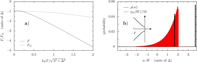
Figure 1: Panel a: Free energy of a two-level-system described by the Hamiltonian (30) with a fixed $\lambda$, as computed in the canonical (Schrödinger-Gibbs) wave function ensemble, Eq. (8), and in the standard Gibbs canonical ensemble. Panel b: Probability histograms of work $w$, Eq. (25), and standard work $W$, Eq. (1), as computed in the canonical (Schrödinger-Gibbs) wave function ensemble, Eq. (8), and in the standard Gibbs canonical ensemble, respectively. The standard work probability $p_{st}(W)$ is rescaled by a factor 10 for better visualization. Inset: sketch of the driving protocol, i.e. a half Landau-Zener sweep. The parameters used are: $\beta=\Delta^{-1},v=\Delta^{2}/\hbar,T=5\hbar/\Delta$.

In Fig. 1.b we report results concerning the work statistics. We considered here a “half” Landau-Zener sweep, i.e., Eq. (30) from time $t=-T$, to time $t=0$, see the inset of Fig. 1.b. The unitary quantum evolution operator can be expressed in terms of special functions [46, 47]. The figure shows both the statistics $p(w)$ originating from the expression of work in Eq. (25) in the canonical wave function ensemble, Eq. (8), and the standard work statistics $p_{st}(W)$ originating from the two-measurement expression of work in Eq. (1) in the standard canonical ensemble $e^{-\beta\hat{H}(\lambda)}/Z_{st}(\beta,\lambda)$. Note the prominent difference that the wave function work pdf $p(w)$ is a smooth function whereas the standard work pdf $p_{st}(W)$ is a discrete sum of 4 Dirac deltas [9] (the two most left peaks of $p_{st}(W)$ are barely visible in Fig. 1.b). Note also that the support of $p(w)$ is smaller than the support of $p_{st}(W)$. Stronger driving (i.e. larger $v$’s) result in broader distributions $p(w)$. The support of $p(w)$ cannot however become wider that that of $p_{st}(W)$, which, independent of $v$, is given by $[-\sqrt{(vT/2)^{2}+\Delta^{2}}-\Delta,\sqrt{(vT/2)^{2}+\Delta^{2}}+\Delta]$.

Notwithstanding their differences both distributions satisfy formally equivalent fluctuation relations. To better clarify this, let us focus on the average exponentiated work. As predicted by the theory and confirmed by our numerical calculation, we have:

$$\langle e^{-\beta w}\rangle=\int dwp(w)e^{-\beta w}=e^{-\beta\Delta F}$$ (36)

$$\langle e^{-\beta W}\rangle_{st}=\int dWp_{st}(W)e^{-\beta W}=e^{-\beta\Delta F_{st}}$$ (37)

That is, both work pdf’s satisfy the Jarzynski equality, each with the free energy calculated in the respective ensemble. Likewise for the Tasaki-Crooks fluctuation theorem.

6 Concluding remarks

We have obtained fluctuation relations for microcanonical and canonical wave function ensembles. They look exactly as the standard relations, but substantially differ from them because they involve a notion of work as the change in the expectation of the energy, rather than the difference of two eigenvalues emerging from quantum collapses. These ensembles in fact have been proposed in a framework where one is interested in the the expectation of quantum observables [30]. As highlighted with the illustrative example, this notion of work gives rise to smooth work probability densities, in stark contrast with the discrete standard probability densities. Also it gives information about the equilibrium “free energy” (“entropy”) as calculated in the canonical (microcanonical) wave function ensemble. These substantially differ from their standard counterpart, see Fig. 1.

Other authors are currently developing alternative formulations of quantum fluctuation relations which do not rely on quantum collapses. Among them is the work of Ref. [48] which presents a study of entropy production based on the Wigner representation of quantum states.

We have expressed some considerations regarding the rational foundations of the wave function ensembles. Further investigation is certainly necessary in order to reach a more satisfactory understanding of the physical basis for these ensembles. One question to be pursued regards the lack of ergodicity of the Hamiltonian flow on the surface of constant energy expectation in the physical Hilbert space, which marks a stark distinction with the classical case. Another important question that deserves further study is whether these ensembles converge to the usual statistical ensembles in some limit, e.g. classical, and/or thermodynamic limit. Experiments will have the final word in regard to their scope of applicability. Certainly they have proved very important in recent advancements in the foundations of quantum statistics [21, 22].

Ackowledgements

This work was supported by the German Excellence Initiative “Nanosystems Initiative Munich (NIM)”.

References

References

- [1] Jarzynski C 1997 Phys. Rev. Lett. 78 2690–2693
- [2] Jarzynski C 2011 Annual Review of Condensed Matter Physics 2 329–351
- [3] Crooks G E 1999 Phys. Rev. E 60 2721–2726
- [4] Kurchan J 2000 arXiv:cond-mat/0007360
- [5] Tasaki H 2000 arXiv:cond-mat/0009244
- [6] Esposito M and Mukamel S 2006 Phys. Rev. E 73 046129
- [7] Talkner P and Hänggi P 2007 J. Phys. A 40 F569–F571
- [8] Esposito M, Harbola U and Mukamel S 2009 Rev. Mod. Phys. 81 1665–1702
- [9] Campisi M, Hänggi P and Talkner P 2011 Rev. Mod. Phys. 83 771–791
- [10] Campisi M, Talkner P and Hänggi P 2010 Phys. Rev. Lett. 105 140601
- [11] Dorner R, Clark S R, Heaney L, Fazio R, Goold J and Vedral V 2013 Phys. Rev. Lett. 110 230601
- [12] Mazzola L, De Chiara G and Paternostro M 2013 Phys. Rev. Lett. 110 230602
- [13] Campisi M, Blattman R, Zueco D, Kohler S and Hänggi P 2013 arXiv:1307.2371
- [14] Batalhão T, Souza A M, Mazzola L, Auccaise R, Oliveira I S, Goold J, De Chiara G, Paternostro M and Serra R M arXiv:1308.3241
- [15] Schrödinger E 1952 Statistical Thermodynamic (Cambridge University Press)
- [16] Khinchin A 1951 Mathematical foundations of quantum statistics (New York: Dover)
- [17] Brody D C and Hughston L P 1998 J. Math. Phys. 39 6502–6508
- [18] Lasinio G J 2000 Invariant Measures under Schrödinger evolution and quantum statistical mechanics (Canadian Mathematical Society Conference Series vol 28) pp 239–242
- [19] Bender C M, Brody D C and Hook D W 2005 J. Phys. A: Math. Theo. 38 L607
- [20] Goldstein S, Lebowitz J, Tumulka R and Zanghì N 2006 J. Stat. Phys. 125 1193–1221
- [21] Goldstein S, Lebowitz J L, Tumulka R and ZanghìN 2006 Phys. Rev. Lett. 96 050403
- [22] Popescu S, Short A J and Winter A 2006 Nat Phys 2 754–758
- [23] Naudts J and der Straeten E V 2006 J. Stat. Mech.: Theory Exp. 2006 P06015
- [24] Brody D C, Hook D W and Hughston L P 2007 Proc. R. Soc. A 463 2021–2030
- [25] Reimann P 2008 Phys. Rev. Lett. 101 190403
- [26] Reimann P 2007 Phys. Rev. Lett. 99 160404
- [27] Fine B V 2009 Phys. Rev. E 80 051130
- [28] Ji K and Fine B V 2011 Phys. Rev. Lett. 107 050401
- [29] Alonso J L, Castro A, Clemente-Gallardo J, Cuchí J C, Echenique P and Falceto F 2011 J. Phys. A: Math. Theo. 44 395004
- [30] Jona-Lasinio G and Presilla C 2006 AIP Conf. Proc. 844 200–205
- [31] Kubo R 1957 J. Phys. Soc. Jpn. 12 570–586
- [32] Strocchi F 1966 Rev. Mod. Phys. 38 36–40
- [33] Huang K 1987 Statistical Mechanics 2nd ed (New York: Wiley)
- [34] Kubo R, Ichimura H, Usui T and Hashitsume N 1965 Statistical Mechanics 6th ed (Amsterdam: North Holland)
- [35] Gallavotti G 1999 Statistical mechanics: a short treatise (Berlin: Springer)
- [36] Campisi M 2007 Physica A 385 501–517
- [37] Campisi M 2005 Stud. Hist. Phil. Mod. Phys. 36 275–290
- [38] Khinchin A 1949 Mathematical foundations of statistical mechanics (New York: Dover)
- [39] Dunkel J and Hilbert S 2013 arXiv:1304.2066
- [40] Cleuren B, Van den Broeck C and Kawai R 2006 Phys. Rev. Lett. 96 050601
- [41] Messiah A 1962 Quantum Mechanics (Amsterdam: North Holland)
- [42] Landau L D 1932 Phys. Z. Sowjetunion 2 46
- [43] Zener C 1932 Proc. R. Soc. A 137 696
- [44] Stückelberg E C G 1932 Helv. Phys. Acta 5 369
- [45] Majorana E 1932 Nuovo Cimento 9 43
- [46] Vitanov N V 1999 Phys. Rev. A 59 988–994
- [47] Campisi M, Talkner P and Hänggi P 2011 Phys. Rev. E 83 041114
- [48] Deffner S 2013 EPL 103 30001