Correlated random features for
fast semi-supervised learning

Abstract

This paper presents Correlated Nyström Views (XNV), a fast semi-supervised algorithm for regression and classification. The algorithm draws on two main ideas. First, it generates two views consisting of computationally inexpensive random features. Second, multiview regression, using Canonical Correlation Analysis (CCA) on unlabeled data, biases the regression towards useful features. It has been shown that CCA regression can substantially reduce variance with a minimal increase in bias if the views contains accurate estimators. Recent theoretical and empirical work shows that regression with random features closely approximates kernel regression, implying that the accuracy requirement holds for random views. We show that XNV consistently outperforms a state-of-the-art algorithm for semi-supervised learning: substantially improving predictive performance and reducing the variability of performance on a wide variety of real-world datasets, whilst also reducing runtime by orders of magnitude.

1 Introduction

As the volume of data collected in the social and natural sciences increases, the computational cost of learning from large datasets has become an important consideration. For learning non-linear relationships, kernel methods achieve excellent performance but naïvely require operations cubic in the number of training points.

Randomization has recently been considered as an alternative to optimization that, surprisingly, can yield comparable generalization performance at a fraction of the computational cost [1, 2]. Random features have been introduced to approximate kernel machines when the number of training examples is very large, rendering exact kernel computation intractable. Among several different approaches, the Nyström method for low-rank kernel approximation [1] exhibits good theoretical properties and empirical performance [3, 4, 5].

A second problem arising with large datasets concerns obtaining labels, which often requires a domain expert to manually assign a label to each instance which can be very expensive – requiring significant investments of both time and money – as the size of the dataset increases. Semi-supervised learning aims to improve prediction by extracting useful structure from the unlabeled data points and using this in conjunction with a function learned on a small number of labeled points.

Contribution.

This paper proposes a new semi-supervised algorithm for regression and classification, Correlated Nyström Views (XNV), that addresses both problems simultaneously. The method consists in essentially two steps. First, we construct two “views” using random features. We investigate two ways of doing so: one based on the Nyström method and another based on random Fourier features (so-called kitchen sinks) [6, 2]. It turns out that the Nyström method almost always outperforms Fourier features by a quite large margin, so we only report these results in the main text.

The second step, following [7], uses Canonical Correlation Analysis (CCA, [8, 9]) to bias the optimization procedure towards features that are correlated across the views. Intuitively, if both views contain accurate estimators, then penalizing uncorrelated features reduces variance without increasing the bias by much. Recent theoretical work by Bach [5] shows that Nyström views can be expected to contain accurate estimators.

We perform an extensive evaluation of XNV on 18 real-world datasets, comparing against a modified version of the SSSL (simple semi-supervised learning) algorithm introduced in [10]. We find that XNV outperforms SSSL by around 10-15% on average, depending on the number of labeled points available, see §3. We also find that the performance of XNV exhibits dramatically less variability than SSSL, with a typical reduction of 30%.

We chose SSSL since it was shown in [10] to outperform a state of the art algorithm, Laplacian Regularized Least Squares [11]. However, since SSSL does not scale up to large sets of unlabeled data, we modify SSSL by introducing a Nyström approximation to improve runtime performance. This reduces runtime by a factor of $\times 1000$ on $N=10,000$ points, with further improvements as $N$ increases. Our approximate version of SSSL outperforms kernel ridge regression (KRR) by $>50\%$ on the 18 datasets on average, in line with the results reported in [10], suggesting that we lose little by replacing the exact SSSL with our approximate implementation.

Related work.

Multiple view learning was first introduced in the co-training method of [12] and has also recently been extended to unsupervised settings [13, 14]. Our algorithm builds on an elegant proposal for multi-view regression introduced in [7]. Surprisingly, despite guaranteeing improved prediction performance under a relatively weak assumption on the views, CCA regression has not been widely used since its proposal – to the best of our knowledge this is first empirical evaluation of multi-view regression’s performance. A possible reason for this is the difficulty in obtaining naturally occurring data equipped with multiple views that can be shown to satisfy the multi-view assumption. We overcome this problem by constructing random views that satisfy the assumption by design.

2 Method

This section introduces XNV, our semi-supervised learning method. The method builds on two main ideas. First, given two equally useful but sufficiently different views on a dataset, penalizing regression using the canonical norm (computed via CCA), can substantially improve performance [7]. The second is the Nyström method for constructing random features [1], which we use to construct the views.

2.1 Multi-view regression

Suppose we have data ${T}=\big{(}({\mathbf{x}}_{1},y_{1}),\ldots,({\mathbf{x}}_{n},y_{n})\big{)}$ for ${\mathbf{x}}_{i}\in{\mathbb{R}}^{D}$ and $y_{i}\in{\mathbb{R}}$, sampled according to joint distribution $P({\mathbf{x}},y)$. Further suppose we have two views on the data

$$\mathbf{z}^{(\nu)}:{\mathbb{R}}^{D}\longrightarrow{\mathcal{H}}^{(\nu)}={\mathbb{R}}^{M}:{\mathbf{x}}\mapsto\mathbf{z}^{(\nu)}({\mathbf{x}})=:\mathbf{z}^{(\nu)}\quad\text{ for }\nu\in\{1,2\}.$$

We make the following assumption about linear regressors which can be learned on these views.

Assumption 1 (Multi-view assumption [7]).

Define mean-squared error loss function $\ell(g,{\mathbf{x}},y)=(g({\mathbf{x}})-y)^{2}$ and let $\operatorname{loss}(g):={\mathbb{E}}_{P}\ell(g({\mathbf{x}}),y)$. Further let $L(Z)$ denote the space of linear maps from a linear space $Z$ to the reals, and define:

$$f^{(\nu)}:=\operatorname*{argmin}_{g\in L({\mathcal{H}}^{(\nu)})}\operatorname{loss}(g)\;\text{ for }\nu\in\{1,2\}\quad{\text{a}nd}\quad f:=\operatorname*{argmin}_{g\in L({\mathcal{H}}^{(1)}\oplus{\mathcal{H}}^{(2)})}\operatorname{loss}(g).$$

The multi-view assumption is that

$$\operatorname{loss}\left(f^{(\nu)}\right)-\operatorname{loss}(f)\leq\epsilon\quad\text{ for }\nu\in\{1,2\}.$$ (1)

In short, the best predictor in each view is within $\epsilon$ of the best overall predictor.

Canonical correlation analysis.

Canonical correlation analysis [8, 9] extends principal component analysis (PCA) from one to two sets of variables. CCA finds bases for the two sets of variables such that the correlation between projections onto the bases are maximized.

The first pair of canonical basis vectors, $\left({{\mathbf{b}}_{1}^{(1)},{\mathbf{b}}_{1}^{(2)}}\right)$ is found by solving:

$$\operatorname*{argmax}_{{\mathbf{b}}^{(1)},{\mathbf{b}}^{(2)}\in{\mathbb{R}}^{M}}\text{corr}\left({{\mathbf{b}}^{(1)\top}\mathbf{z}^{(1)},{\mathbf{b}}^{(2)\top}\mathbf{z}^{(2)}}\right).$$ (2)

Subsequent pairs are found by maximizing correlations subject to being orthogonal to previously found pairs. The result of performing CCA is two sets of bases, ${\mathbf{B}}^{(\nu)}=\left[{{\mathbf{b}}_{1}^{(\nu)},\ldots,{\mathbf{b}}_{M}^{(\nu)}}\right]$ for $\nu\in\{1,2\}$, such that the projection of $\mathbf{z}^{(\nu)}$ onto ${\mathbf{B}}^{(\nu)}$ which we denote $\bar{\mathbf{z}}^{(\nu)}$ satisfies

1. Orthogonality: ${\mathbb{E}}_{T}\big{[}\bar{\mathbf{z}}^{(\nu)\top}_{j}\bar{\mathbf{z}}^{(\nu)}_{k}]=\delta_{jk}$, where $\delta_{jk}$ is the Kronecker delta, and

2. Correlation: ${\mathbb{E}}_{T}\big{[}\bar{\mathbf{z}}^{(1)\top}_{j}\bar{\mathbf{z}}^{(2)}_{k}\big{]}=\lambda_{j}\cdot\delta_{jk}$ where w.l.o.g. we assume $1\geq\lambda_{1}\geq\lambda_{2}\geq\cdots\geq 0$.

$\lambda_{j}$ is referred to as the $j^{th}$ canonical correlation coefficient.

Definition 1 (canonical norm).

Given vector $\bar{\mathbf{z}}^{(\nu)}$ in the canonical basis, define its canonical norm as

$$\|\bar{\mathbf{z}}^{(\nu)}\|_{CCA}:=\sqrt{\sum_{j=1}^{D}\frac{1-\lambda_{j}}{\lambda_{j}}\left(\bar{z}^{(\nu)}_{j}\right)^{2}}.$$

Canonical ridge regression.

Assume we observe $n$ pairs of views coupled with real valued labels $\left\{{\mathbf{z}_{i}^{(1)},\mathbf{z}_{i}^{(2)},y_{i}}\right\}_{i=1}^{n}$, canonical ridge regression finds coefficients $\widehat{{\boldsymbol{{{\beta}}}}}^{(\nu)}=\left[{\widehat{{{\beta}}}_{1}^{(\nu)},\ldots,\widehat{{{\beta}}}_{M}^{(\nu)}}\right]^{\top}$ such that

$$\widehat{{\boldsymbol{{{\beta}}}}}^{(\nu)}:=\operatorname*{argmin}_{{\boldsymbol{{{\beta}}}}}\frac{1}{n}\sum_{i=1}^{n}\left(y_{i}-{{\boldsymbol{{{\beta}}}}}^{(\nu)~{}\top}\bar{\mathbf{z}}^{(\nu)}_{i}\right)^{2}+\|{\boldsymbol{{{\beta}}}}^{(\nu)}\|_{CCA}^{2}.$$ (3)

The resulting estimator, referred to as the canonical shrinkage estimator, is

$$\widehat{{{\beta}}}^{(\nu)}_{j}=\frac{\lambda_{j}}{n}\sum_{i=1}^{n}\bar{\mathbf{z}}^{(\nu)}_{i,j}y_{i}.$$ (4)

Penalizing with the canonical norm biases the optimization towards features that are highly correlated across the views. Good regressors exist in both views by Assumption 1. Thus, intuitively, penalizing uncorrelated features significantly reduces variance, without increasing the bias by much. More formally:

Theorem 1 (canonical ridge regression, [7]).

Assume ${\mathbb{E}}[y^{2}|{\mathbf{x}}]\leq 1$ and that Assumption 1 holds. Let $f^{(\nu)}_{\widehat{{\boldsymbol{{{\beta}}}}}}$ denote the estimator constructed with the canonical shrinkage estimator, Eq. (4), on training set ${T}$, and let $f$ denote the best linear predictor across both views. For $\nu\in\{1,2\}$ we have

$${\mathbb{E}}_{T}[\operatorname{loss}(f_{\widehat{{\boldsymbol{{{\beta}}}}}}^{(\nu)})]-\operatorname{loss}(f)\leq 5\epsilon+\frac{\sum_{j=1}^{M}\lambda_{j}^{2}}{n}$$

where the expectation is with respect to training sets ${T}$ sampled from $P({\mathbf{x}},y)$.

The first term, $5\epsilon$, bounds the bias of the canonical estimator, whereas the second, $\frac{1}{n}\sum\lambda_{j}^{2}$ bounds the variance. The $\sum\lambda_{j}^{2}$ can be thought of as a measure of the “intrinsic dimensionality” of the unlabeled data, which controls the rate of convergence. If the canonical correlation coefficients decay sufficiently rapidly, then the increase in bias is more than made up for by the decrease in variance.

2.2 Constructing random views

We construct two views satisfying Assumption 1 in expectation, see Theorem 3 below. To ensure our method scales to large sets of unlabeled data, we use random features generated using the Nyström method [1].

Suppose we have data $\{{\mathbf{x}}_{i}\}_{i=1}^{N}$. When $N$ is very large, constructing and manipulating the $N\times N$ Gram matrix $\left[{{\mathbf{K}}}\right]_{ii^{\prime}}=\left\langle{\phi({\mathbf{x}}_{i}),\phi({\mathbf{x}}_{i^{\prime}})}\right\rangle=\kappa({\mathbf{x}}_{i},{\mathbf{x}}_{i^{\prime}})$ is computationally expensive. Where here, $\phi({\mathbf{x}})$ defines a mapping from ${\mathbb{R}}^{D}$ to a high dimensional feature space and $\kappa(\cdot,\cdot)$ is a positive semi-definite kernel function.

The idea behind random features is to instead define a lower-dimensional mapping, $\mathbf{z}({\mathbf{x}}_{i}):{\mathbb{R}}^{D}\rightarrow{\mathbb{R}}^{M}$ through a random sampling scheme such that $\left[{{\mathbf{K}}}\right]_{ii^{\prime}}\approx\mathbf{z}({\mathbf{x}}_{i})^{\top}\mathbf{z}({\mathbf{x}}_{i^{\prime}})$ [15, 6]. Thus, using random features, non-linear functions in ${\mathbf{x}}$ can be learned as linear functions in $\mathbf{z}({\mathbf{x}})$ leading to significant computational speed-ups. Here we give a brief overview of the Nyström method, which uses random subsampling to approximate the Gram matrix.

The Nyström method.

Fix an $M\ll N$ and randomly (uniformly) sample a subset $\mathcal{M}=\{\hat{{\mathbf{x}}}_{i}\}_{i=1}^{M}$ of $M$ points from the data $\{{\mathbf{x}}_{i}\}_{i=1}^{N}$. Let $\widehat{\mathbf{K}}$ denote the Gram matrix $[\widehat{\mathbf{K}}]_{ii^{\prime}}$ where $i,i^{\prime}\in{\mathcal{M}}$. The Nyström method [1, 3] constructs a low-rank approximation to the Gram matrix as

$${\mathbf{K}}\approx\tilde{\mathbf{K}}:=\sum_{i=1}^{N}\sum_{i^{\prime}=1}^{N}\left[{\kappa({\mathbf{x}}_{i},\hat{{\mathbf{x}}}_{1}),\ldots,\kappa({\mathbf{x}}_{i},\hat{{\mathbf{x}}}_{M})}\right]\widehat{{\mathbf{K}}}^{\dagger}\left[{\kappa({\mathbf{x}}_{i^{\prime}},\hat{{\mathbf{x}}}_{1}),\ldots,\kappa({\mathbf{x}}_{i^{\prime}},\hat{{\mathbf{x}}}_{M})}\right]^{\top},$$ (5)

where $\widehat{{\mathbf{K}}}^{\dagger}\in{\mathbb{R}}^{M\times M}$ is the pseudo-inverse of $\widehat{\mathbf{K}}$. Vectors of random features can be constructed as

$$\mathbf{z}({\mathbf{x}}_{i})=\widehat{{\mathbf{D}}}^{-1/2}\widehat{{\mathbf{V}}}^{\top}\left[{\kappa({\mathbf{x}}_{i},\hat{{\mathbf{x}}}_{1}),\ldots,\kappa({\mathbf{x}}_{i},\hat{{\mathbf{x}}}_{M})}\right]^{\top},$$

where the columns of $\widehat{{\mathbf{V}}}$ are the eigenvectors of $\widehat{{\mathbf{K}}}$ with $\widehat{{\mathbf{D}}}$ the diagonal matrix whose entries are the corresponding eigenvalues. Constructing features in this way reduces the time complexity of learning a non-linear prediction function from $O(N^{3})$ to $O(N)$ [15].

An alternative perspective on the Nyström approximation, that will be useful below, is as follows. Consider integral operators

$$L_{N}[f](\cdot):=\frac{1}{N}\sum_{i=1}^{N}\kappa({\mathbf{x}}_{i},\cdot)f({\mathbf{x}}_{i})\quad\text{ and }\quad L_{M}[f](\cdot):=\frac{1}{M}\sum_{i=1}^{M}\kappa({\mathbf{x}}_{i},\cdot)f({\mathbf{x}}_{i}),$$ (6)

and introduce Hilbert space $\hat{{\mathcal{H}}}=\text{span}\left\{\hat{\varphi}_{1},\ldots,\hat{\varphi}_{r}\right\}$ where $r$ is the rank of $\widehat{\mathbf{K}}$ and the $\hat{\varphi}_{i}$ are the first $r$ eigenfunctions of $L_{M}$. Then the following proposition shows that using the Nyström approximation is equivalent to performing linear regression in the feature space (“view”) $\mathbf{z}:{\mathcal{X}}\rightarrow\hat{{\mathcal{H}}}$ spanned by the eigenfunctions of linear operator $L_{M}$ in Eq. (6):

Proposition 2 (random Nyström view, [3]).

Solving

$$\min_{{\mathbf{w}}\in{\mathbb{R}}^{r}}\frac{1}{N}\sum_{i=1}^{N}\ell({\mathbf{w}}^{\top}\mathbf{z}({\mathbf{x}}_{i}),y_{i})+\frac{\gamma}{2}\|{\mathbf{w}}\|^{2}_{2}$$ (7)

is equivalent to solving

$$\min_{f\in\hat{{\mathcal{H}}}}\frac{1}{N}\sum_{i=1}^{N}\ell(f({\mathbf{x}}_{i}),y_{i})+\frac{\gamma}{2}\|f\|^{2}_{{\mathcal{H}}_{\kappa}}.$$ (8)

2.3 The proposed algorithm: Correlated Nyström Views (XNV)

Algorithm 1 details our approach to semi-supervised learning based on generating two views consisting of Nyström random features and penalizing features which are weakly correlated across views. The setting is that we have labeled data $\{{\mathbf{x}}_{i},y_{i}\}_{i=1}^{n}$ and a large amount of unlabeled data $\{{\mathbf{x}}_{i}\}_{i=n+1}^{N}$.

Algorithm 1 Correlated Nyström Views (XNV).

Input:  Labeled data: $\{{\mathbf{x}}_{i},y_{i}\}_{i=1}^{n}$ and unlabeled data: $\{{\mathbf{x}}_{i}\}_{i=n+1}^{N}$

1:  Generate features. Sample $\hat{{\mathbf{x}}}_{1},\ldots,\hat{{\mathbf{x}}}_{2M}$ uniformly from the dataset, compute the eigendecompositions of the sub-sampled kernel matrices $\hat{{\mathbf{K}}}^{(1)}$ and $\hat{{\mathbf{K}}}^{(2)}$ which are constructed from the samples $1,\ldots,M$ and $M+1,\ldots,2M$ respectively, and featurize the input:

$$\quad\mathbf{z}^{(\nu)}({\mathbf{x}}_{i})\leftarrow\hat{{\mathbf{D}}}^{(\nu),-1/2}\hat{{\mathbf{V}}}^{(\nu)\top}\left[{\kappa({\mathbf{x}}_{i},\hat{{\mathbf{x}}}_{1}),\ldots,\kappa({\mathbf{x}}_{i},\hat{{\mathbf{x}}}_{M})}\right]^{\top}\text{ for }\nu\in\{1,2\}.$$

2:  Unlabeled data. Compute CCA bases ${\mathbf{B}}^{(1)}$, ${\mathbf{B}}^{(2)}$ and canonical correlations $\lambda_{1},\ldots,\lambda_{M}$ for the two views and set $\bar{\mathbf{z}}_{i}\leftarrow{\mathbf{B}}^{(1)}\mathbf{z}^{(1)}({\mathbf{x}}_{i}).$

3:  Labeled data. Solve

$$\widehat{{\boldsymbol{{{\beta}}}}}=\operatorname*{argmin}_{{\boldsymbol{{{\beta}}}}}\frac{1}{n}\sum_{i=1}^{n}\ell\left({{\boldsymbol{{{\beta}}}}^{\top}\bar{\mathbf{z}}_{i},y_{i}}\right)+\|{\boldsymbol{{{\beta}}}}\|^{2}_{CCA}+\gamma\|{\boldsymbol{{{\beta}}}}\|_{2}^{2}~{}.$$ (9)

Output:  $\widehat{{\boldsymbol{{{\beta}}}}}$

Step 1 generates a set of random features. The next two steps implement multi-view regression using the randomly generated views $\mathbf{z}^{(1)}({\mathbf{x}})$ and $\mathbf{z}^{(2)}({\mathbf{x}})$. Eq. (9) yields a solution for which unimportant features are heavily downweighted in the CCA basis without introducing an additional tuning parameter. The further penalty on the $\ell_{2}$ norm (in the CCA basis) is introduced as a practical measure to control the variance of the estimator $\widehat{{\boldsymbol{{{\beta}}}}}$ which can become large if there are many highly correlated features (i.e. the ratio $\frac{1-\lambda_{j}}{\lambda_{j}}\approx 0$ for large $j$). In practice most of the shrinkage is due to the CCA norm: cross-validation obtains optimal values of $\gamma$ in the range $[0.00001,0.1]$.

Computational complexity.

XNV is extremely fast. Nyström sampling, step 1, reduces the $O(N^{3})$ operations required for kernel learning to $O(N)$. Computing the CCA basis, step 2, using standard algorithms is in $O(NM^{2})$. However, we reduce the runtime to $O(NM)$ by applying a recently proposed randomized CCA algorithm of [16]. Finally, step 3 is a computationally cheap linear program on $n$ samples and $M$ features.

Performance guarantees.

The quality of the kernel approximation in (5) has been the subject of detailed study in recent years leading to a number of strong empirical and theoretical results [3, 4, 5, 15]. Recent work of Bach [5] provides theoretical guarantees on the quality of Nyström estimates in the fixed design setting that are relevant to our approach.

Theorem 3 (Nyström generalization bound, [5]).

Let $\xi\in{\mathbb{R}}^{N}$ be a random vector with finite variance and zero mean, $\mathbf{y}=\left[{y_{1},\ldots,y_{N}}\right]^{\top}$, and define smoothed estimate $\hat{\mathbf{y}}_{\text{kernel}}:=(\mathbf{K}+N\gamma\mathbf{I})^{-1}\mathbf{K}(\mathbf{y}+\xi)$ and smoothed Nyström estimate $\hat{\mathbf{y}}_{\text{Nystr\"{o}m}}:=(\tilde{\mathbf{K}}+N\gamma\mathbf{I})^{-1}\tilde{\mathbf{K}}(\mathbf{y}+\xi)$, both computed by minimizing the MSE with ridge penalty $\gamma$. Let $\eta\in(0,1)$. For sufficiently large $M$ (depending on $\eta$, see [5]), we have

$${\mathbb{E}}_{\mathcal{M}}{\mathbb{E}}_{\xi}\left[\|\mathbf{y}-\hat{\mathbf{y}}_{\text{Nystr\"{o}m}}\|^{2}_{2}\right]\leq(1+4\eta)\cdot{\mathbb{E}}_{\xi}\left[\|\mathbf{y}-\hat{\mathbf{y}}_{\text{kernel}}\|^{2}_{2}\right]$$

where ${\mathbb{E}}_{\mathcal{M}}$ refers to the expectation over subsampled columns used to construct $\tilde{\mathbf{K}}$.

In short, the best smoothed estimators in the Nyström views are close to the optimal smoothed estimator. Since the kernel estimate is consistent, $\operatorname{loss}(f)\rightarrow 0$ as $n\rightarrow\infty$. Thus, Assumption 1 holds in expectation and the generalization performance of XNV is controlled by Theorem 1.

Random Fourier Features.

An alternative approach to constructing random views is to use Fourier features instead of Nyström features in Step 1. We refer to this approach as Correlated Kitchen Sinks (XKS) after [2]. It turns out that the performance of XKS is consistently worse than XNV, in line with the detailed comparison presented in [3]. We therefore do not discuss Fourier features in the main text, see §SI.3 for details on implementation and experimental results.

2.4 A fast approximation to SSSL

The SSSL (simple semi-supervised learning) algorithm proposed in [10] finds the first $s$ eigenfunctions $\phi_{i}$ of the integral operator $L_{N}$ in Eq. (6) and then solves

$$\operatorname*{argmin}_{{\mathbf{w}}\in{\mathbb{R}}^{s}}\sum_{i=1}^{n}\left(\sum_{j=1}^{s}w_{j}\phi_{k}({\mathbf{x}}_{i})-y_{i}\right)^{2},$$ (10)

where $s$ is set by the user. SSSL outperforms Laplacian Regularized Least Squares [11], a state of the art semi-supervised learning method, see [10]. It also has good generalization guarantees under reasonable assumptions on the distribution of eigenvalues of $L_{N}$. However, since SSSL requires computing the full $N\times N$ Gram matrix, it is extremely computationally intensive for large $N$. Moreover, tuning $s$ is difficult since it is discrete.

We therefore propose SSSL_M, an approximation to SSSL. First, instead of constructing the full Gram matrix, we construct a Nyström approximation by sampling $M$ points from the labeled and unlabeled training set. Second, instead of thresholding eigenfunctions, we use the easier to tune ridge penalty which penalizes directions proportional to the inverse square of their eigenvalues [18].

As justification, note that Proposition 2 states that the Nyström approximation to kernel regression actually solves a ridge regression problem in the span of the eigenfunctions of $\hat{L}_{M}$. As $M$ increases, the span of $\hat{L}_{M}$ tends towards that of $L_{N}$ [15]. We will also refer to the Nyström approximation to SSSL using $2M$ features as SSSL_2M. See experiments below for further discussion of the quality of the approximation.

3 Experiments

Setup.

We evaluate the performance of XNV on 18 real-world datasets, see Table 1. The datasets cover a variety of regression (denoted by R) and two-class classification (C) problems. The sarcos dataset involves predicting the joint position of a robot arm; following convention we report results on the 1st, 5th and 7th joint positions.

Table 1: Datasets used for evaluation.

Set	Name	Task	N	D	Set	Name	Task	N	D
1	abalone	C	$2,089$	$6$	10	elevators4	R	$8,752$	$18$
2	adult2	C	$32,561$	$14$	11	HIVa	C	$21,339$	$1,617$
3	ailerons	R	$7,154$	$40$	12	house4	R	$11,392$	$16$
4	bank84	C	$4,096$	$8$	13	ibn Sina3	C	$10,361$	$92$
5	bank324	C	$4,096$	$32$	14	orange3	C	$25,000$	$230$
6	cal housing4	R	$10,320$	$8$	15	sarcos 1	R	$44,484$	$21$
7	census2	R	$18,186$	$119$	16	sarcos 55	R	$44,484$	$21$
8	CPU2	R	$6,554$	$21$	17	sarcos 75	R	$44,484$	$21$
9	CT2	R	$30,000$	$385$	18	sylva3	C	$72,626$	$216$

The SSSL algorithm was shown to exhibit state-of-the-art performance over fully and semi-supervised methods in scenarios where few labeled training examples are available [10]. However, as discussed in §2.2, due to its computational cost we compare the performance of XNV to the Nyström approximations SSSL_M and SSSL_2M.

We used a Gaussian kernel for all datasets. We set the kernel width, $\sigma$ and the $\ell_{2}$ regularisation strength, $\gamma$, for each method using 5-fold cross validation with $1000$ labeled training examples. We trained all methods using a squared error loss function, $\ell(f({\mathbf{x}}_{i}),y_{i})=(f({\mathbf{x}}_{i})-y_{i})^{2}$, with $M=200$ random features, and $n=100,150,200,\ldots,1000$ randomly selected training examples.

Runtime performance.

The SSSL algorithm of [10] is not computationally feasible on large datasets, since it has time complexity $O(N^{3})$. For illustrative purposes, we report run times in seconds of the SSSL algorithm against SSSL_M and XNV on three datasets of different sizes.

runtimes	bank8	cal housing	sylva
SSSL	$72$s	$2300$s	-
SSSL2M	$0.3$s	$0.6$s	$24$s
XNV	$0.9$s	$1.3$s	$26$s

For the cal housing dataset, XNV exhibits an almost $1800\times$ speed up over SSSL. For the largest dataset, sylva, exact SSSL is computationally intractable. Importantly, the computational overhead of XNV over SSSL_2M is small.

Generalization performance.

We report on the prediction performance averaged over 100 experiments. For regression tasks we report on the mean squared error (MSE) on the testing set normalized by the variance of the test output. For classification tasks we report the percentage of the test set that was misclassified.

The table below shows the improvement in performance of XNV over SSSL_M and SSSL_2M (taking whichever performs better out of $M$ or $2M$ on each dataset), averaged over all 18 datasets. Observe that XNV is considerably more accurate and more robust than SSSL_M.

XNV vs SSSLM/2M	$n=100$	$n=200$	$n=300$	$n=400$	$n=500$
Avg reduction in error	11%	16%	15%	12%	9%
Avg reduction in std err	15%	30%	31%	33%	30%

The reduced variability is to be expected from Theorem 1.

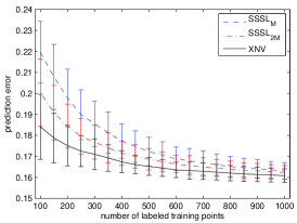
(a) adult

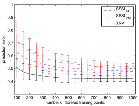
(b) cal housing

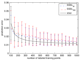
(c) census

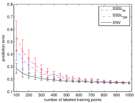
(d) elevators

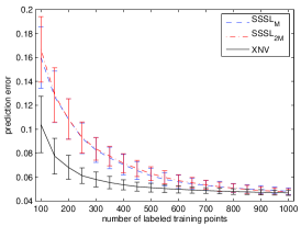
(e) ibn Sina

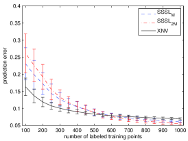
(f) sarcos 5

Figure 1: Comparison of mean prediction error and standard deviation on a selection of datasets.

Table 2 presents more detailed comparison of performance for individual datasets when $n=200,400$. The plots in Figure 1 shows a representative comparison of mean prediction errors for several datasets when $n=100,\ldots,1000$. Error bars represent one standard deviation. Observe that XNV almost always improves prediction accuracy and reduces variance compared with SSSL_M and SSSL_2M when the labeled training set contains between 100 and 500 labeled points. A complete set of results is provided in §SI.1.

Discussion of SSSL_M.

Our experiments show that going from $M$ to $2M$ does not improve generalization performance in practice. This suggests that when there are few labeled points, obtaining a more accurate estimate of the eigenfunctions of the kernel does not necessarily improve predictive performance. Indeed, when more random features are added, stronger regularization is required to reduce the influence of uninformative features, this also has the effect of downweighting informative features. This suggests that the low rank approximation SSSL_M to SSSL suffices.

Finally, §SI.2 compares the performance of SSSL_M and XNV to fully supervised kernel ridge regression (KRR). We observe dramatic improvements, between 48% and 63%, consistent with the results observed in [10] for the exact SSSL algorithm.

Random Fourier features.

Nyström features significantly outperform Fourier features, in line with observations in [3]. The table below shows the relative improvement of XNV over XKS:

XNV vs XKS	$n=100$	$n=200$	$n=300$	$n=400$	$n=500$
Avg reduction in error	30%	28%	26%	25%	24%
Avg reduction in std err	36%	44%	34%	37%	36%

Further results and discussion for XKS are included in the supplementary material.

Table 2: Performance (normalized MSE/classification error rate). Standard errors in parentheses.

set	SSSLM	SSSL2M	XNV	set	SSSLM	SSSL2M	XNV
$n=200$
1	$0.054$ $(0.005)$	$0.055$ $(0.006)$	${\bf 0.053}$ $({\bf 0.004})$	10	$0.309$ $(0.059)$	$0.358$ $(0.077)$	${\bf 0.226}$ $({\bf 0.020})$
2	$0.198$ $(0.014)$	$0.184$ $(0.010)$	${\bf 0.175}$ $({\bf 0.010})$	11	$0.146$ $(0.048)$	$0.072$ $(0.024)$	${\bf 0.036}$ $({\bf 0.001})$
3	$0.218$ $(0.016)$	$0.231$ $(0.020)$	${\bf 0.213}$ $({\bf 0.016})$	12	${\bf 0.761}$ $({\bf 0.075})$	$0.787$ $(0.091)$	$0.792$ $(0.100)$
4	${\bf 0.558}$ $({\bf 0.027})$	$0.567$ $(0.029)$	$0.561$ $(0.030)$	13	$0.109$ $(0.017)$	$0.109$ $(0.017)$	${\bf 0.068}$ $({\bf 0.010})$
5	$0.058$ $(0.004)$	$0.060$ $(0.005)$	${\bf 0.055}$ $({\bf 0.003})$	14	$0.019$ $(0.001)$	$0.019$ $(0.001)$	${\bf 0.019}$ $({\bf 0.000})$
6	$0.567$ $(0.081)$	$0.634$ $(0.103)$	${\bf 0.459}$ $({\bf 0.045})$	15	$0.076$ $(0.008)$	$0.078$ $(0.009)$	${\bf 0.071}$ $({\bf 0.006})$
7	$0.020$ $(0.012)$	$0.022$ $(0.014)$	${\bf 0.019}$ $({\bf 0.005})$	16	$0.172$ $(0.032)$	$0.192$ $(0.036)$	${\bf 0.119}$ $({\bf 0.014})$
8	$0.395$ $(0.395)$	$0.463$ $(0.414)$	${\bf 0.263}$ $({\bf 0.352})$	17	$0.041$ $(0.004)$	$0.043$ $(0.005)$	${\bf 0.040}$ $({\bf 0.004})$
9	$0.437$ $(0.096)$	$0.367$ $(0.060)$	${\bf 0.222}$ $({\bf 0.015})$	18	$0.036$ $(0.007)$	$0.039$ $(0.007)$	${\bf 0.028}$ $({\bf 0.009})$
$n=400$
1	$0.051$ $(0.003)$	$0.052$ $(0.003)$	${\bf 0.050}$ $({\bf 0.002})$	10	$0.218$ $(0.022)$	$0.233$ $(0.027)$	${\bf 0.192}$ $({\bf 0.010})$
2	$0.177$ $(0.008)$	$0.172$ $(0.006)$	${\bf 0.167}$ $({\bf 0.005})$	11	$0.051$ $(0.009)$	$0.122$ $(0.031)$	${\bf 0.036}$ $({\bf 0.001})$
3	$0.199$ $(0.011)$	$0.209$ $(0.013)$	${\bf 0.193}$ $({\bf 0.010})$	12	${\bf 0.691}$ $({\bf 0.040})$	$0.701$ $(0.051)$	$0.709$ $(0.058)$
4	$0.517$ $(0.018)$	$0.527$ $(0.019)$	${\bf 0.510}$ $({\bf 0.016})$	13	$0.070$ $(0.009)$	$0.072$ $(0.008)$	${\bf 0.054}$ $({\bf 0.004})$
5	$0.050$ $(0.003)$	$0.051$ $(0.003)$	${\bf 0.050}$ $({\bf 0.002})$	14	$0.019$ $(0.001)$	$0.019$ $(0.001)$	${\bf 0.019}$ $({\bf 0.000})$
6	$0.513$ $(0.055)$	$0.555$ $(0.063)$	${\bf 0.432}$ $({\bf 0.036})$	15	$0.059$ $(0.004)$	$0.060$ $(0.005)$	${\bf 0.057}$ $({\bf 0.003})$
7	$0.019$ $(0.010)$	$0.021$ $(0.012)$	${\bf 0.014}$ $({\bf 0.003})$	16	$0.105$ $(0.014)$	$0.106$ $(0.014)$	${\bf 0.090}$ $({\bf 0.007})$
8	$0.209$ $(0.171)$	$0.286$ $(0.248)$	${\bf 0.110}$ $({\bf 0.107})$	17	${\bf 0.032}$ $({\bf 0.002})$	$0.033$ $(0.003)$	${\bf 0.032}$ $({\bf 0.002})$
9	$0.249$ $(0.024)$	$0.304$ $(0.037)$	${\bf 0.201}$ $({\bf 0.013})$	18	$0.029$ $(0.006)$	$0.032$ $(0.005)$	${\bf 0.023}$ $({\bf 0.006})$

4 Conclusion

We have introduced the XNV algorithm for semi-supervised learning. By combining two randomly generated views of Nyström features via an efficient implementation of CCA, XNV outperforms the prior state-of-the-art, SSSL, by 10-15% (depending on the number of labeled points) on average over 18 datasets. Furthermore, XNV is over 3 orders of magnitude faster than SSSL on medium sized datasets ($N=10,000$) with further gains as $N$ increases. An interesting research direction is to investigate using the recently developed deep CCA algorithm, which extracts higher order correlations between views [19], as a preprocessing step.

In this work we use a uniform sampling scheme for the Nyström method for computational reasons since it has been shown to perform well empirically relative to more expensive schemes [20]. Since CCA gives us a criterion by which to measure the important of random features, in the future we aim to investigate active sampling schemes based on canonical correlations which may yield better performance by selecting the most informative indices to sample.

Acknowledgements.

We thank Haim Avron for help with implementing randomized CCA and Patrick Pletscher for drawing our attention to the Nyström method.

Supplementary Information

SI.1 Complete XNV results

Table 3: Performance (normalized MSE/classification error rate). Standard errors in parentheses.

set	SSSLM	SSSL2M	XNV	set	SSSLM	SSSL2M	XNV
$n=100$
1	${\bf 0.058}$ $({\bf 0.008})$	$0.060$ $(0.009)$	$0.059$ $(0.008)$	10	$0.439$ $(0.088)$	$0.545$ $(0.121)$	${\bf 0.286}$ $({\bf 0.040})$
2	$0.220$ $(0.015)$	$0.200$ $(0.016)$	${\bf 0.184}$ $({\bf 0.016})$	11	$0.064$ $(0.025)$	$0.054$ $(0.015)$	${\bf 0.037}$ $({\bf 0.001})$
3	${\bf 0.249}$ $({\bf 0.024})$	$0.263$ $(0.028)$	$0.255$ $(0.029)$	12	${\bf 0.825}$ $({\bf 0.114})$	$0.864$ $(0.144)$	$0.895$ $(0.163)$
4	${\bf 0.651}$ $({\bf 0.063})$	$0.666$ $(0.070)$	$0.691$ $(0.082)$	13	$0.160$ $(0.026)$	$0.167$ $(0.027)$	${\bf 0.104}$ $({\bf 0.024})$
5	$0.068$ $(0.008)$	$0.076$ $(0.012)$	${\bf 0.061}$ $({\bf 0.005})$	14	$0.020$ $(0.003)$	$0.020$ $(0.003)$	${\bf 0.019}$ $({\bf 0.000})$
6	$0.628$ $(0.122)$	$0.718$ $(0.153)$	${\bf 0.504}$ $({\bf 0.074})$	15	$0.104$ $(0.015)$	$0.104$ $(0.016)$	${\bf 0.095}$ $({\bf 0.013})$
7	${\bf 0.029}$ $({\bf 0.016})$	$0.031$ $(0.019)$	$0.036$ $(0.020)$	16	$0.231$ $(0.047)$	$0.261$ $(0.057)$	${\bf 0.163}$ $({\bf 0.026})$
8	$0.691$ $(0.603)$	$0.751$ $(0.659)$	${\bf 0.568}$ $({\bf 0.613})$	17	$0.058$ $(0.010)$	$0.061$ $(0.011)$	${\bf 0.056}$ $({\bf 0.009})$
9	$0.488$ $(0.123)$	$0.367$ $(0.073)$	${\bf 0.276}$ $({\bf 0.047})$	18	$0.042$ $(0.009)$	$0.043$ $(0.009)$	${\bf 0.036}$ $({\bf 0.011})$
$n=200$
1	$0.054$ $(0.005)$	$0.055$ $(0.006)$	${\bf 0.053}$ $({\bf 0.004})$	10	$0.309$ $(0.059)$	$0.358$ $(0.077)$	${\bf 0.226}$ $({\bf 0.020})$
2	$0.198$ $(0.014)$	$0.184$ $(0.010)$	${\bf 0.175}$ $({\bf 0.010})$	11	$0.146$ $(0.048)$	$0.072$ $(0.024)$	${\bf 0.036}$ $({\bf 0.001})$
3	$0.218$ $(0.016)$	$0.231$ $(0.020)$	${\bf 0.213}$ $({\bf 0.016})$	12	${\bf 0.761}$ $({\bf 0.075})$	$0.787$ $(0.091)$	$0.792$ $(0.100)$
4	${\bf 0.558}$ $({\bf 0.027})$	$0.567$ $(0.029)$	$0.561$ $(0.030)$	13	$0.109$ $(0.017)$	$0.109$ $(0.017)$	${\bf 0.068}$ $({\bf 0.010})$
5	$0.058$ $(0.004)$	$0.060$ $(0.005)$	${\bf 0.055}$ $({\bf 0.003})$	14	$0.019$ $(0.001)$	$0.019$ $(0.001)$	${\bf 0.019}$ $({\bf 0.000})$
6	$0.567$ $(0.081)$	$0.634$ $(0.103)$	${\bf 0.459}$ $({\bf 0.045})$	15	$0.076$ $(0.008)$	$0.078$ $(0.009)$	${\bf 0.071}$ $({\bf 0.006})$
7	$0.020$ $(0.012)$	$0.022$ $(0.014)$	${\bf 0.019}$ $({\bf 0.005})$	16	$0.172$ $(0.032)$	$0.192$ $(0.036)$	${\bf 0.119}$ $({\bf 0.014})$
8	$0.395$ $(0.395)$	$0.463$ $(0.414)$	${\bf 0.263}$ $({\bf 0.352})$	17	$0.041$ $(0.004)$	$0.043$ $(0.005)$	${\bf 0.040}$ $({\bf 0.004})$
9	$0.437$ $(0.096)$	$0.367$ $(0.060)$	${\bf 0.222}$ $({\bf 0.015})$	18	$0.036$ $(0.007)$	$0.039$ $(0.007)$	${\bf 0.028}$ $({\bf 0.009})$
$n=300$
1	$0.052$ $(0.004)$	$0.053$ $(0.004)$	${\bf 0.051}$ $({\bf 0.003})$	10	$0.250$ $(0.031)$	$0.275$ $(0.040)$	${\bf 0.205}$ $({\bf 0.014})$
2	$0.185$ $(0.011)$	$0.177$ $(0.008)$	${\bf 0.171}$ $({\bf 0.007})$	11	$0.074$ $(0.020)$	$0.105$ $(0.032)$	${\bf 0.036}$ $({\bf 0.001})$
3	$0.206$ $(0.012)$	$0.217$ $(0.015)$	${\bf 0.200}$ $({\bf 0.012})$	12	${\bf 0.719}$ $({\bf 0.052})$	$0.736$ $(0.067)$	$0.744$ $(0.083)$
4	$0.531$ $(0.020)$	$0.540$ $(0.021)$	${\bf 0.526}$ $({\bf 0.020})$	13	$0.083$ $(0.010)$	$0.084$ $(0.009)$	${\bf 0.058}$ $({\bf 0.006})$
5	$0.053$ $(0.004)$	$0.055$ $(0.004)$	${\bf 0.052}$ $({\bf 0.003})$	14	$0.019$ $(0.002)$	$0.019$ $(0.002)$	${\bf 0.019}$ $({\bf 0.000})$
6	$0.535$ $(0.065)$	$0.585$ $(0.079)$	${\bf 0.444}$ $({\bf 0.039})$	15	$0.066$ $(0.005)$	$0.067$ $(0.006)$	${\bf 0.062}$ $({\bf 0.004})$
7	$0.020$ $(0.010)$	$0.022$ $(0.013)$	${\bf 0.016}$ $({\bf 0.003})$	16	$0.126$ $(0.020)$	$0.133$ $(0.022)$	${\bf 0.100}$ $({\bf 0.009})$
8	$0.270$ $(0.216)$	$0.370$ $(0.333)$	${\bf 0.152}$ $({\bf 0.199})$	17	$0.035$ $(0.003)$	$0.037$ $(0.004)$	${\bf 0.035}$ $({\bf 0.002})$
9	$0.304$ $(0.038)$	$0.352$ $(0.055)$	${\bf 0.207}$ $({\bf 0.013})$	18	$0.032$ $(0.006)$	$0.035$ $(0.007)$	${\bf 0.025}$ $({\bf 0.006})$
$n=400$
1	$0.051$ $(0.003)$	$0.052$ $(0.003)$	${\bf 0.050}$ $({\bf 0.002})$	10	$0.218$ $(0.022)$	$0.233$ $(0.027)$	${\bf 0.192}$ $({\bf 0.010})$
2	$0.177$ $(0.008)$	$0.172$ $(0.006)$	${\bf 0.167}$ $({\bf 0.005})$	11	$0.051$ $(0.009)$	$0.122$ $(0.031)$	${\bf 0.036}$ $({\bf 0.001})$
3	$0.199$ $(0.011)$	$0.209$ $(0.013)$	${\bf 0.193}$ $({\bf 0.010})$	12	${\bf 0.691}$ $({\bf 0.040})$	$0.701$ $(0.051)$	$0.709$ $(0.058)$
4	$0.517$ $(0.018)$	$0.527$ $(0.019)$	${\bf 0.510}$ $({\bf 0.016})$	13	$0.070$ $(0.009)$	$0.072$ $(0.008)$	${\bf 0.054}$ $({\bf 0.004})$
5	$0.050$ $(0.003)$	$0.051$ $(0.003)$	${\bf 0.050}$ $({\bf 0.002})$	14	$0.019$ $(0.001)$	$0.019$ $(0.001)$	${\bf 0.019}$ $({\bf 0.000})$
6	$0.513$ $(0.055)$	$0.555$ $(0.063)$	${\bf 0.432}$ $({\bf 0.036})$	15	$0.059$ $(0.004)$	$0.060$ $(0.005)$	${\bf 0.057}$ $({\bf 0.003})$
7	$0.019$ $(0.010)$	$0.021$ $(0.012)$	${\bf 0.014}$ $({\bf 0.003})$	16	$0.105$ $(0.014)$	$0.106$ $(0.014)$	${\bf 0.090}$ $({\bf 0.007})$
8	$0.209$ $(0.171)$	$0.286$ $(0.248)$	${\bf 0.110}$ $({\bf 0.107})$	17	${\bf 0.032}$ $({\bf 0.002})$	$0.033$ $(0.003)$	${\bf 0.032}$ $({\bf 0.002})$
9	$0.249$ $(0.024)$	$0.304$ $(0.037)$	${\bf 0.201}$ $({\bf 0.013})$	18	$0.029$ $(0.006)$	$0.032$ $(0.005)$	${\bf 0.023}$ $({\bf 0.006})$
$n=500$
1	$0.051$ $(0.002)$	$0.051$ $(0.003)$	${\bf 0.050}$ $({\bf 0.002})$	10	$0.202$ $(0.017)$	$0.214$ $(0.020)$	${\bf 0.185}$ $({\bf 0.008})$
2	$0.172$ $(0.007)$	$0.169$ $(0.005)$	${\bf 0.165}$ $({\bf 0.004})$	11	$0.043$ $(0.005)$	$0.092$ $(0.018)$	${\bf 0.036}$ $({\bf 0.001})$
3	$0.194$ $(0.008)$	$0.202$ $(0.010)$	${\bf 0.188}$ $({\bf 0.007})$	12	${\bf 0.675}$ $({\bf 0.035})$	$0.680$ $(0.044)$	$0.686$ $(0.047)$
4	$0.508$ $(0.012)$	$0.517$ $(0.014)$	${\bf 0.499}$ $({\bf 0.011})$	13	$0.061$ $(0.006)$	$0.063$ $(0.006)$	${\bf 0.051}$ $({\bf 0.004})$
5	$0.048$ $(0.002)$	$0.049$ $(0.002)$	${\bf 0.048}$ $({\bf 0.002})$	14	${\bf 0.019}$ $({\bf 0.000})$	${\bf 0.019}$ $({\bf 0.000})$	${\bf 0.019}$ $({\bf 0.000})$
6	$0.503$ $(0.052)$	$0.541$ $(0.060)$	${\bf 0.427}$ $({\bf 0.034})$	15	$0.055$ $(0.003)$	$0.055$ $(0.004)$	${\bf 0.054}$ $({\bf 0.002})$
7	$0.017$ $(0.007)$	$0.018$ $(0.007)$	${\bf 0.014}$ $({\bf 0.002})$	16	$0.089$ $(0.010)$	$0.088$ $(0.010)$	${\bf 0.083}$ $({\bf 0.005})$
8	$0.167$ $(0.137)$	$0.241$ $(0.235)$	${\bf 0.098}$ $({\bf 0.097})$	17	${\bf 0.030}$ $({\bf 0.002})$	$0.030$ $(0.002)$	$0.031$ $(0.001)$
9	$0.222$ $(0.017)$	$0.259$ $(0.027)$	${\bf 0.196}$ $({\bf 0.011})$	18	$0.027$ $(0.004)$	$0.029$ $(0.005)$	${\bf 0.022}$ $({\bf 0.005})$

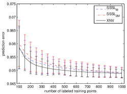
(a) abalone

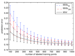
(b) adult

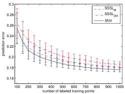
(c) ailerons

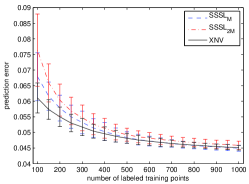
(d) bank8

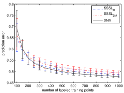
(e) bank32

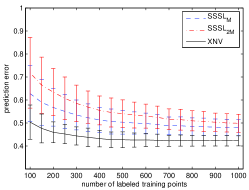
(f) cal housing

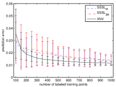
(g) census

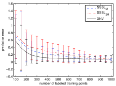
(h) CPU

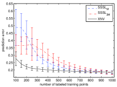
(i) CT

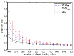
(j) elevators

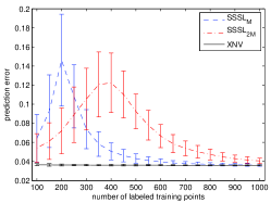
(k) HIVa

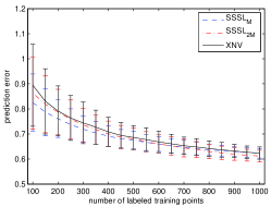
(l) house

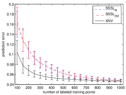
(m) ibn Sina

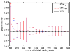
(n) orange

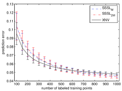
(o) sarcos 1

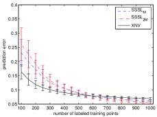
(p) sarcos 5

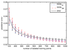
(q) sarcos 7

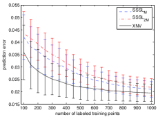
(r) sylva

Figure 2: Comparison of mean prediction error and standard deviation on all 18 datasets.

SI.2 Comparison with Kernel Ridge Regression

We compare SSSL_M and XNV to kernel ridge regression (KRR). The table below reports the percentage improvement in mean error of both of these methods against KRR, averaged over the 18 datasets according to the experimental procedure detailed in §3. Parameters $\sigma$ (kernel width) and $\gamma$ (ridge penalty) for KRR were chosen by 5-fold cross validation. We observe that both SSSL_M and XNV far outperform KRR, by $50-60\%$. Importantly, this shows our approximation to SSSL far outperforms the fully supervised baseline.

SSSLM and XNV vs KRR	$n=100$	$n=200$	$n=300$	$n=400$	$n=500$
Avg reduction in error for SSSLM	48%	52%	56%	58%	60%
Avg reduction in error for XNV	56%	62%	63%	63%	63%

SI.3 Random Fourier features

Random Fourier features are a method for approximating shift invariant kernels [6], i.e. where $\kappa({\mathbf{x}}_{i},{\mathbf{x}}_{i^{\prime}})=\kappa({\mathbf{x}}_{i}-{\mathbf{x}}_{i^{\prime}})$. Such a kernel function can be represented in terms of its inverse Fourier transform as $\kappa({\mathbf{x}}_{i}-{\mathbf{x}}_{i^{\prime}})=\int_{{\mathbb{R}}^{D}}P(\boldsymbol{\omega})e^{j\boldsymbol{\omega}^{\top}\left({{\mathbf{x}}_{i}-{\mathbf{x}}_{i^{\prime}}}\right)}$. $P(\boldsymbol{\omega})$ is the Fourier transform of $\kappa$ which is guaranteed to be a proper probability distribution and so for real-valued features $\kappa({\mathbf{x}}_{i},{\mathbf{x}}_{i^{\prime}})$ can be equivalently interpreted as ${\mathbb{E}}_{\boldsymbol{\omega}}\left[{\mathbf{z}({\mathbf{x}}_{i})^{\top}\mathbf{z}({\mathbf{x}}_{i^{\prime}})}\right]$ where $\mathbf{z}({\mathbf{x}}_{i})=\frac{1}{\sqrt{2}}\cos(\boldsymbol{\omega}^{\top}{\mathbf{x}}_{i}+b)$ . Replacing the expectation by the sample average leads to a scheme for constructing random features. In particular, a Gaussian kernel of width $\sigma$ has a Fourier transform which is also Gaussian. Sampling $\boldsymbol{\omega}_{m}\sim{\mathcal{N}}(0,2\sigma\mathbf{I}_{D})$ and $b_{m}\sim\text{Unif}\left[{-\pi,\pi}\right]$, we can then construct features whose inner product approximates this kernel as $\mathbf{z}_{i}=\frac{1}{\sqrt{M}}\left[{\cos(\boldsymbol{\omega}_{1}^{\top}{\mathbf{x}}_{i}+b_{1}),\ldots,\cos(\boldsymbol{\omega}_{M}^{\top}{\mathbf{x}}_{i}+b_{M})}\right]$.

It was recently shown how both random Fourier features the Nyström approximation could be cast in the same framework [3]. A major difference between the methods lies in the sampling scheme employed. Random Fourier features are constructed in a data independent fashion which makes them extremely cheap to compute. Nyström features are constructed in a data dependent way which leads to improved performance but, in the case of semi-supervised learning, more expensive since we need to evaluate the approximate kernel for all unlabeled points we wish to use.

Algorithm 2 details Correlated Kitchen Sinks (XKS). This algorithm generates random views using the random Fourier features procedure in step 1. Steps 2 and 3 proceed exactly as in Algorithm 1.

Algorithm 2 Correlated Kitchen Sinks (XKS).

Input:  Labeled data: $\{{\mathbf{x}}_{i},y_{i}\}_{i=1}^{n}$ and unlabeled data: $\{{\mathbf{x}}_{i}\}_{i=n+1}^{N}$

1:  Generate features. Draw $\omega_{1},\ldots\omega_{2K}$ i.i.d. from $P$ and featurize the input:

$$\quad\mathbf{z}^{(1)}_{i}\leftarrow \left[{\phi({\mathbf{x}}_{i};\boldsymbol{\omega}_{1}),\ldots,\phi({\mathbf{x}}_{i};\boldsymbol{\omega}_{M})}\right],$$

$$\quad\mathbf{z}^{(2)}_{i}\leftarrow \left[{\phi({\mathbf{x}}_{i};\boldsymbol{\omega}_{M+1}),\ldots,\phi({\mathbf{x}}_{i};\boldsymbol{\omega}_{2M})}\right].$$

2:  Unlabeled data. Compute CCA bases ${\mathbf{B}}^{(1)}$, ${\mathbf{B}}^{(2)}$ and canonical correlations $\lambda_{1},\ldots,\lambda_{M}$ for the two views and set $\bar{\mathbf{z}}_{i}\leftarrow{\mathbf{B}}^{(1)}\mathbf{z}^{(1)}_{i}.$

3:  Labeled data. Solve

$$\widehat{{\boldsymbol{{{\beta}}}}}=\min_{{\boldsymbol{{{\beta}}}}}\frac{1}{n}\sum_{i=1}^{n}\ell\left({{\boldsymbol{{{\beta}}}}^{\top}\bar{\mathbf{z}}_{i},y_{i}}\right)+\|{\boldsymbol{{{\beta}}}}\|^{2}_{CCA}+\gamma\|{\boldsymbol{{{\beta}}}}\|_{2}^{2}~{}.$$ (11)

Output:  $\widehat{{\boldsymbol{{{\beta}}}}}$

It can be shown that, with sufficiently many features, views constructed via random Fourier features contain good approximations to a large class of functions with high probability, see main theorem of [2]. We do not provide details, since XKS is consistently outperformed by XNV in practice.

SI.4 Complete XKS results

For completeness we report on the performance of the XKS algorithm. We use the same experimental setup as in Section 3. We compare the performance of XKS against a linear machine learned using $M$ and $2M$ random Fourier features respectively.

Table 4: Average performance of XKS against RFF_M/2M on 18 datasets.

XKS vs RFFM/2M	$n=100$	$n=200$	$n=300$	$n=400$	$n=500$
Avg reduction in error	15%	30%	34%	31%	28%
Avg reduction in std err	-1%	35%	47%	43%	44%

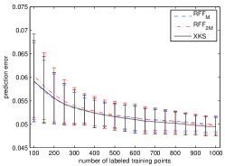
(a) abalone

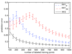
(b) adult

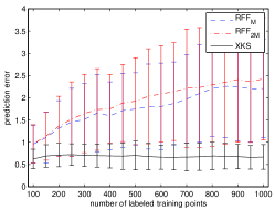
(c) ailerons

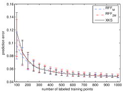
(d) bank8

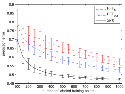
(e) bank32

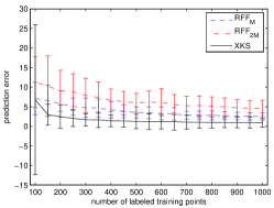
(f) cal housing

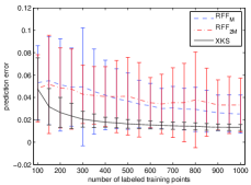
(g) census

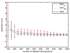
(h) CPU

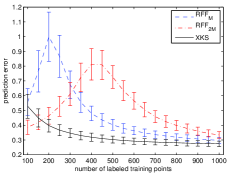
(i) CT

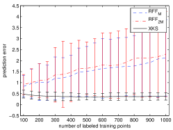
(j) elevators

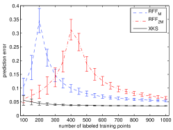
(k) HIVa

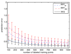
(l) house

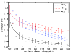
(m) ibn Sina

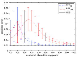
(n) orange

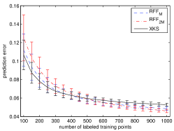
(o) sarcos 1

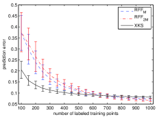
(p) sarcos 5

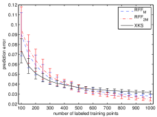
(q) sarcos 7

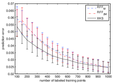
(r) sylva

Figure 3: Comparison of mean prediction error and standard deviation on all 18 datasets.

Table 4 shows the performance improvement of XKS over RFF_M/2M, averaged across the 18 datasets. Table 6 compares the prediction error and standard deviation for each of the datasets individually. Figure 3 shows the performance across the full range of values of $n$ for all datasets. The relative performance of XKS against RFF_M and RFF_2M follows the same trend seen in Section 3, suggesting that CCA-based regression consistently improves on regression across single and joint views.

Table 5: Number of datasets (out of 18) on which XNV outperforms XKS.

$n=100$	$n=200$	$n=300$	$n=400$	$n=500$
16	16	15	16	16

Finally, Table 5 compares the performance of correlated Nyström features against correlated kitchen sinks. XNV typically outperforms XKS on 16 out of 18 datasets; with XKS only ever outperforming XNV on bank8, house and orange. Since XNV almost always outperforms XKS, we only discuss Nyström features in the main text.

Table 6: Performance of XKS (normalized MSE/classification error rate). Standard errors in parentheses.

set	RFFM	RFF2M	XKS	set	RFFM	RFF2M	XKS
$n=100$
1	${\bf 0.059}$ $({\bf 0.008})$	$0.060$ $(0.009)$	$0.059$ $(0.009)$	10	$0.829$ $(0.490)$	$0.913$ $(0.457)$	${\bf 0.478}$ $({\bf 0.176})$
2	$0.349$ $(0.031)$	$0.325$ $(0.032)$	${\bf 0.274}$ $({\bf 0.024})$	11	$0.106$ $(0.030)$	$0.060$ $(0.013)$	${\bf 0.056}$ $({\bf 0.018})$
3	$0.956$ $(0.421)$	$0.963$ $(0.428)$	${\bf 0.626}$ $({\bf 0.220})$	12	$1.085$ $(0.267)$	$1.240$ $(0.374)$	${\bf 0.849}$ $({\bf 0.101})$
4	$0.778$ $(0.089)$	$0.793$ $(0.092)$	${\bf 0.700}$ $({\bf 0.077})$	13	$0.183$ $(0.027)$	$0.183$ $(0.027)$	${\bf 0.154}$ $({\bf 0.023})$
5	${\bf 0.096}$ $({\bf 0.021})$	$0.108$ $(0.028)$	$0.116$ $(0.030)$	14	$0.067$ $(0.045)$	$0.047$ $(0.030)$	${\bf 0.019}$ $({\bf 0.000})$
6	$7.091$ $(4.146)$	$11.320$ $(6.500)$	${\bf 6.801}$ $({\bf 19.194})$	15	$0.112$ $(0.017)$	$0.125$ $(0.025)$	${\bf 0.107}$ $({\bf 0.016})$
7	$0.053$ $(0.033)$	$0.048$ $(0.030)$	${\bf 0.048}$ $({\bf 0.028})$	16	$0.373$ $(0.079)$	$0.376$ $(0.089)$	${\bf 0.205}$ $({\bf 0.039})$
8	$1.813$ $(2.438)$	$2.062$ $(3.915)$	${\bf 1.155}$ $({\bf 1.379})$	17	$0.090$ $(0.022)$	$0.095$ $(0.023)$	${\bf 0.074}$ $({\bf 0.012})$
9	$0.556$ $(0.092)$	${\bf 0.386}$ $({\bf 0.048})$	$0.528$ $(0.082)$	18	$0.059$ $(0.009)$	$0.056$ $(0.009)$	${\bf 0.054}$ $({\bf 0.007})$
$n=200$
1	${\bf 0.055}$ $({\bf 0.005})$	$0.056$ $(0.006)$	$0.056$ $(0.005)$	10	$1.026$ $(0.837)$	$1.094$ $(0.766)$	${\bf 0.402}$ $({\bf 0.177})$
2	$0.403$ $(0.028)$	$0.338$ $(0.026)$	${\bf 0.219}$ $({\bf 0.012})$	11	$0.346$ $(0.044)$	$0.087$ $(0.024)$	${\bf 0.044}$ $({\bf 0.006})$
3	$1.316$ $(0.619)$	$1.359$ $(0.675)$	${\bf 0.713}$ $({\bf 0.262})$	12	$0.935$ $(0.142)$	$1.059$ $(0.203)$	${\bf 0.776}$ $({\bf 0.071})$
4	$0.674$ $(0.041)$	$0.724$ $(0.051)$	${\bf 0.561}$ $({\bf 0.031})$	13	$0.159$ $(0.017)$	$0.157$ $(0.017)$	${\bf 0.113}$ $({\bf 0.015})$
5	${\bf 0.070}$ $({\bf 0.012})$	$0.073$ $(0.013)$	$0.073$ $(0.013)$	14	$0.109$ $(0.053)$	$0.070$ $(0.040)$	${\bf 0.019}$ $({\bf 0.000})$
6	$5.731$ $(3.367)$	$9.037$ $(5.248)$	${\bf 2.454}$ $({\bf 2.998})$	15	$0.082$ $(0.010)$	$0.090$ $(0.014)$	${\bf 0.078}$ $({\bf 0.008})$
7	$0.051$ $(0.041)$	$0.049$ $(0.036)$	${\bf 0.027}$ $({\bf 0.013})$	16	$0.239$ $(0.052)$	$0.266$ $(0.067)$	${\bf 0.136}$ $({\bf 0.017})$
8	$0.922$ $(1.119)$	$0.938$ $(0.783)$	${\bf 0.643}$ $({\bf 0.974})$	17	$0.059$ $(0.010)$	$0.064$ $(0.011)$	${\bf 0.051}$ $({\bf 0.006})$
9	$0.999$ $(0.167)$	$0.464$ $(0.057)$	${\bf 0.397}$ $({\bf 0.043})$	18	$0.053$ $(0.006)$	$0.053$ $(0.006)$	${\bf 0.044}$ $({\bf 0.006})$
$n=300$
1	${\bf 0.053}$ $({\bf 0.003})$	$0.054$ $(0.004)$	$0.054$ $(0.004)$	10	$1.197$ $(0.969)$	$1.354$ $(1.238)$	${\bf 0.375}$ $({\bf 0.201})$
2	$0.315$ $(0.021)$	$0.374$ $(0.021)$	${\bf 0.200}$ $({\bf 0.009})$	11	$0.146$ $(0.023)$	$0.139$ $(0.034)$	${\bf 0.040}$ $({\bf 0.003})$
3	$1.513$ $(0.804)$	$1.646$ $(0.878)$	${\bf 0.706}$ $({\bf 0.248})$	12	$0.869$ $(0.103)$	$0.964$ $(0.151)$	${\bf 0.739}$ $({\bf 0.053})$
4	$0.636$ $(0.033)$	$0.705$ $(0.040)$	${\bf 0.523}$ $({\bf 0.018})$	13	$0.145$ $(0.014)$	$0.145$ $(0.013)$	${\bf 0.095}$ $({\bf 0.009})$
5	${\bf 0.060}$ $({\bf 0.006})$	$0.062$ $(0.007)$	$0.060$ $(0.006)$	14	$0.048$ $(0.019)$	$0.105$ $(0.046)$	${\bf 0.019}$ $({\bf 0.000})$
6	$4.769$ $(2.468)$	$7.871$ $(4.393)$	${\bf 1.660}$ $({\bf 1.549})$	15	$0.069$ $(0.006)$	$0.073$ $(0.008)$	${\bf 0.067}$ $({\bf 0.005})$
7	$0.050$ $(0.053)$	$0.043$ $(0.026)$	${\bf 0.021}$ $({\bf 0.007})$	16	$0.165$ $(0.027)$	$0.181$ $(0.030)$	${\bf 0.113}$ $({\bf 0.010})$
8	$0.699$ $(0.437)$	$0.789$ $(0.511)$	${\bf 0.416}$ $({\bf 0.241})$	17	$0.046$ $(0.006)$	$0.049$ $(0.007)$	${\bf 0.043}$ $({\bf 0.003})$
9	$0.673$ $(0.094)$	$0.611$ $(0.078)$	${\bf 0.346}$ $({\bf 0.031})$	18	$0.046$ $(0.007)$	$0.045$ $(0.007)$	${\bf 0.039}$ $({\bf 0.006})$
$n=400$
1	${\bf 0.052}$ $({\bf 0.003})$	$0.053$ $(0.003)$	$0.052$ $(0.003)$	10	$1.311$ $(0.927)$	$1.466$ $(1.328)$	${\bf 0.364}$ $({\bf 0.172})$
2	$0.264$ $(0.013)$	$0.401$ $(0.020)$	${\bf 0.190}$ $({\bf 0.008})$	11	$0.099$ $(0.013)$	$0.313$ $(0.038)$	${\bf 0.038}$ $({\bf 0.002})$
3	$1.596$ $(0.760)$	$1.752$ $(0.771)$	${\bf 0.695}$ $({\bf 0.273})$	12	$0.815$ $(0.087)$	$0.894$ $(0.118)$	${\bf 0.714}$ $({\bf 0.041})$
4	$0.605$ $(0.025)$	$0.675$ $(0.032)$	${\bf 0.504}$ $({\bf 0.014})$	13	$0.133$ $(0.011)$	$0.139$ $(0.011)$	${\bf 0.087}$ $({\bf 0.008})$
5	$0.056$ $(0.005)$	$0.058$ $(0.005)$	${\bf 0.056}$ $({\bf 0.005})$	14	$0.029$ $(0.007)$	$0.111$ $(0.038)$	${\bf 0.019}$ $({\bf 0.000})$
6	$4.214$ $(2.123)$	$6.632$ $(2.862)$	${\bf 1.394}$ $({\bf 1.533})$	15	${\bf 0.063}$ $({\bf 0.004})$	$0.065$ $(0.006)$	$0.063$ $(0.004)$
7	$0.042$ $(0.031)$	$0.041$ $(0.027)$	${\bf 0.018}$ $({\bf 0.004})$	16	$0.129$ $(0.017)$	$0.139$ $(0.022)$	${\bf 0.102}$ $({\bf 0.008})$
8	$0.605$ $(0.382)$	$0.695$ $(0.553)$	${\bf 0.350}$ $({\bf 0.181})$	17	$0.040$ $(0.004)$	$0.041$ $(0.004)$	${\bf 0.039}$ $({\bf 0.003})$
9	$0.480$ $(0.049)$	$0.812$ $(0.106)$	${\bf 0.318}$ $({\bf 0.027})$	18	$0.040$ $(0.006)$	$0.039$ $(0.006)$	${\bf 0.035}$ $({\bf 0.005})$
$n=500$
1	$0.052$ $(0.003)$	$0.052$ $(0.003)$	${\bf 0.052}$ $({\bf 0.003})$	10	$1.514$ $(1.130)$	$1.650$ $(1.195)$	${\bf 0.355}$ $({\bf 0.142})$
2	$0.237$ $(0.010)$	$0.362$ $(0.018)$	${\bf 0.183}$ $({\bf 0.006})$	11	$0.080$ $(0.009)$	$0.188$ $(0.027)$	${\bf 0.037}$ $({\bf 0.002})$
3	$1.747$ $(0.815)$	$1.923$ $(0.976)$	${\bf 0.703}$ $({\bf 0.323})$	12	$0.782$ $(0.069)$	$0.847$ $(0.097)$	${\bf 0.698}$ $({\bf 0.031})$
4	$0.583$ $(0.023)$	$0.653$ $(0.028)$	${\bf 0.494}$ $({\bf 0.010})$	13	$0.124$ $(0.011)$	$0.133$ $(0.010)$	${\bf 0.082}$ $({\bf 0.007})$
5	$0.053$ $(0.004)$	$0.055$ $(0.005)$	${\bf 0.053}$ $({\bf 0.003})$	14	$0.023$ $(0.003)$	$0.079$ $(0.022)$	${\bf 0.019}$ $({\bf 0.000})$
6	$3.515$ $(1.416)$	$5.977$ $(2.419)$	${\bf 1.231}$ $({\bf 1.848})$	15	${\bf 0.058}$ $({\bf 0.004})$	$0.059$ $(0.005)$	$0.060$ $(0.003)$
7	$0.037$ $(0.025)$	$0.041$ $(0.035)$	${\bf 0.016}$ $({\bf 0.004})$	16	$0.108$ $(0.013)$	$0.114$ $(0.015)$	${\bf 0.095}$ $({\bf 0.007})$
8	$0.533$ $(0.408)$	$0.536$ $(0.505)$	${\bf 0.307}$ $({\bf 0.132})$	17	$0.036$ $(0.003)$	${\bf 0.036}$ $({\bf 0.004})$	$0.037$ $(0.002)$
9	$0.403$ $(0.037)$	$0.726$ $(0.077)$	${\bf 0.303}$ $({\bf 0.023})$	18	$0.036$ $(0.006)$	$0.035$ $(0.006)$	${\bf 0.032}$ $({\bf 0.005})$

References

• [1] Williams C, Seeger M: Using the Nyström method to speed up kernel machines. In NIPS 2001.
• [2] Rahimi A, Recht B: Weighted sums of random kitchen sinks: Replacing minimization with randomization in learning. In Adv in Neural Information Processing Systems (NIPS) 2008.
• [3] Yang T, Li YF, Mahdavi M, Jin R, Zhou ZH: Nyström Method vs Random Fourier Features: A Theoretical and Empirical Comparison. In NIPS 2012.
• [4] Gittens A, Mahoney MW: Revisiting the Nyström method for improved large-scale machine learning. In ICML 2013.
• [5] Bach F: Sharp analysis of low-rank kernel approximations. In COLT 2013.
• [6] Rahimi A, Recht B: Random Features for Large-Scale Kernel Machines. In Adv in Neural Information Processing Systems 2007.
• [7] Kakade S, Foster DP: Multi-view Regression Via Canonical Correlation Analysis. In Computational Learning Theory (COLT) 2007.
• [8] Hotelling H: Relations between two sets of variates. Biometrika 1936, 28:312–377.
• [9] Hardoon DR, Szedmak S, Shawe-Taylor J: Canonical Correlation Analysis: An Overview with Application to Learning Methods. Neural Comp 2004, 16(12):2639–2664.
• [10] Ji M, Yang T, Lin B, Jin R, Han J: A Simple Algorithm for Semi-supervised Learning with Improved Generalization Error Bound. In ICML 2012.
• [11] Belkin M, Niyogi P, Sindhwani V: Manifold regularization: A geometric framework for learning from labeled and unlabeled examples. JMLR 2006, 7:2399–2434.
• [12] Blum A, Mitchell T: Combining labeled and unlabeled data with co-training. In COLT 1998.
• [13] Chaudhuri K, Kakade SM, Livescu K, Sridharan K: Multiview clustering via Canonical Correlation Analysis. In ICML 2009.
• [14] McWilliams B, Montana G: Multi-view predictive partitioning in high dimensions. Statistical Analysis and Data Mining 2012, 5:304–321.
• [15] Drineas P, Mahoney MW: On the Nyström Method for Approximating a Gram Matrix for Improved Kernel-Based Learning. JMLR 2005, 6:2153–2175.
• [16] Avron H, Boutsidis C, Toledo S, Zouzias A: Efficient Dimensionality Reduction for Canonical Correlation Analysis. In ICML 2013.
• [17] Hsu D, Kakade S, Zhang T: An Analysis of Random Design Linear Regression. In COLT 2012.
• [18] Dhillon PS, Foster DP, Kakade SM, Ungar LH: A Risk Comparison of Ordinary Least Squares vs Ridge Regression. Journal of Machine Learning Research 2013, 14:1505–1511.
• [19] Andrew G, Arora R, Bilmes J, Livescu K: Deep Canonical Correlation Analysis. In ICML 2013.
• [20] Kumar S, Mohri M, Talwalkar A: Sampling methods for the Nyström method. JMLR 2012, 13:981–1006.