Variable and clause elimination for
LTL satisfiability checking

Abstract

We study preprocessing techniques for clause normal forms of LTL formulas. Applying the mechanism of labelled clauses enables us to reinterpret LTL satisfiability as a set of purely propositional problems and thus to transfer simplification ideas from SAT to LTL. We demonstrate this by adapting variable and clause elimination, a very effective preprocessing technique used by modern SAT solvers. Our experiments confirm that even in the temporal setting substantial reductions in formula size and subsequent decrease of solver runtime can be achieved.

1 Introduction

Linear temporal logic (LTL) is a modal logic with modalities referring to time [13]. Traditionally, it finds its use in formal verification of reactive systems where it serves as a specification language for expressing the system’s desired behavior. The specifications are subsequently checked against a model of the system during the process of model checking [3]. More recently, the importance of LTL satisfiability checking is becoming recognized [14, 16], where the task is to decide whether a given LTL formula has a model at all. This is, for instance, essential for assuring quality of formal specifications [12]. Satisfiability checking of LTL is a computationally difficult task, in fact a PSPACE-complete one [17], and thus techniques for improving solving methods are of practical importance.

One possibility for speeding up the checking lies in simplifying the input formula before the actual decision method is started. In the context of resolution-based methods for LTL satisfiability [8, 18], on which we focus here, formulas are first translated into a clause normal form. Simplification then means reducing the number of clauses and variables while preserving satisfiability of the formula. Such a preprocessing step may have a significant positive impact on the subsequent running time.

In this paper we take inspiration from the SAT community where a technique called variable and clause elimination [5] has been shown to be particularly effective. It combines exhaustive application of the resolution rule over selected variables with subsumption and other reductions. Our main contribution lies in showing that variable and clause elimination can be adapted from SAT to the setting of LTL. This is quite non-trivial, because LTL normal forms consist of temporal clauses, which are bound to specific temporal contexts and so their interactions in inferences and reductions need to be carefully controlled.

A general method for reducing LTL satisfiability to the purely propositional setting has been introduced in [18]. There, the existence of a model of an LTL formula is shown to be equivalent to satisfiability of one of infinitely many potentially infinite standard clause sets. These are, however, finitely represented with the help of labels, which allows for an effective transfer of resolution-based reasoning techniques from propositional logic to LTL. In this paper, we extend the ideas of [18] to adapt variable and clause elimination. An additional label component is needed to justify elimination in its general form, but we prove it can be dispensed with after the elimination process.

Our exposition starts in Sect. 2, where we describe our version of clause normal form of LTL formulas, which we call LTL-specification. Specifications are a particular refinement of the Separated Normal Form [7], which can be seen as concise descriptions of Büchi automata. This observation, which is of independent interest, represents another contribution of this paper. The mechanism of labelled clauses itself is introduced in Sect. 3 and utilized for variable and clause elimination in Sect. 4. Practical potential of our method is demonstrated in Sect. 5, where we describe the effect of the simplification on runtimes of two resolution-based LTL provers over an extensive set of benchmark problems. In Sect. 6 we follow the connection to Büchi automata to discuss related work, and we conclude in Sect. 7 by mentioning possibilities for future work.

2 Preliminaries

We assume the reader is familiar with propositional logic and the syntax and semantics of LTL. LTL formulas are built over a given signature $\Sigma=\{p,q,r,\ldots\}$ of propositional variables using propositional connectives $\neg,\land,\lor,\ldots$, and temporal operators $\bigcirc,\Box,\Diamond,\mathsf{U},\ldots$ Propositional clauses, denoted $C,D$, possibly with subscripts, are sets of literals understood as disjunctions. A propositional valuation is a mapping $W:\Sigma\rightarrow\{0,1\}$. We write $W\models C$ if a valuation $W$ propositionally satisfies a clause $C$. An interpretation of an LTL formula is an infinite sequence of valuations $(W_{i})_{i\in\mathbb{N}}$, in this context also referred to as states.

In order to talk about two neighboring states at once we introduce a disjoint copy of the basic signature $\Sigma^{\prime}=\{p^{\prime},q^{\prime},r^{\prime},\ldots\}$. Given a clause $C$ over $\Sigma$, we write $C^{\prime}$ to denote its obvious counterpart over $\Sigma^{\prime}$. For a valuation $W$ over $\Sigma$ let $W^{\prime}$ denote the valuation over $\Sigma^{\prime}$ that behaves on primed symbols in the same way as $W$ does on unprimed ones. We therefore have $W\models C$ if and only if $W^{\prime}\models C^{\prime}$ for any such $W$ and $C$. If $W_{1}$ and $W_{2}$ are two valuations over $\Sigma$, we let $[W_{1},W_{2}]$ denote the joined valuation $W_{1}\cup(W_{2})^{\prime}:\Sigma\cup\Sigma^{\prime}\rightarrow\{0,1\}$. Such a valuation is needed to evaluate clauses over the joined signature $\Sigma\cup\Sigma^{\prime}$.

Most resolution-based approaches to satisfiability checking first translate the input formula into a certain normal form. In the context of LTL, the Separated Normal Form (SNF) developed by Fisher [7] has proven to be very useful. It is obtained from an LTL formula by applying transformations that 1) introduce new variables as names for complex subformulas, 2) remove temporal operators by expanding their fixpoint definitions, 3) apply classical style rewrite operations to obtain a result which is clausal, i.e. represented by a top-level conjunction of temporal clauses, which are disjunctive in nature. The whole transformation preserves satisfiability of the input formula and it is ensured that the result does not grow in size by more than a linear factor [8].

In this paper we use a particular refinement of SNF which we call LTL-specification [18]. To obtain a specification, a general SNF is first normalized further by using the ideas of [4]. In particular, we transform the so called conditional eventuality clauses to unconditional ones and then reduce the potentially multiple (unconditional) eventuality clauses to just one eventuality clause. Finally, to obtain a compact representation, we explicitly sort the clauses into three categories, strip them off the temporal operators and write them down using standard propositional clauses instead. The semantics is preserved as it now follows from the context. Even after these refinements the result is linearly bounded in size and equisatisfiable with respect to the original formula.

Definition 1

An LTL-specification is a quadruple $\mathcal{S}=(\Sigma,I,T,G)$ such that

• $\Sigma$ is a finite propositional signature,

• $I$ is a set of initial clauses $C_{i}$ over the signature $\Sigma$,

• $T$ is a set of step clauses $C_{t}\lor(D_{t})^{\prime}$ over the joined signature $\Sigma\cup\Sigma^{\prime}$,

• $G$ is a set of goal clauses $C_{g}$ over the signature $\Sigma$.

The initial and step clauses are directly translated from SNF. The goal clauses all together express the single eventuality obtained in the previous step. This generalization (from a single goal clause) is for free and appears to make the definition conceptually cleaner. Intuitively, specification stands for the LTL formula

$$\left(\bigwedge C_{i}\right)\land\Box\left(\bigwedge(C_{t}\lor\bigcirc D_{t})\right)\land\Box\Diamond\left(\bigwedge C_{g}\right)\enspace,$$

which directly translates to the following formal definition.

Definition 2

An interpretation $(W_{i})_{i\in\mathbb{N}}$ is a model of $\mathcal{S}=(\Sigma,I,T,G)$ if

1. for every $C_{i}\in I$, $W_{0}\models C_{i}$,

2. for every $i\in\mathbb{N}$ and every $C_{t}\lor(D_{t})^{\prime}\in T$, $[W_{i},W_{i+1}]\models C_{t}\lor(D_{t})^{\prime}$, and

3. there are infinitely many indices $j$ such that for every $C_{g}\in G$, $W_{j}\models C_{g}$.

An LTL-specification $\mathcal{S}$ is satisfiable if it has a model.

Remark 1

We close this section with an interesting observation relating our approach to LTL satisfiability to explicit methods based on automata. It is well known (see e.g. [9]) that for any LTL formula $\varphi$ there is a Büchi automaton $\mathcal{A}_{\varphi}$ recognizing models of $\varphi$, i.e. an automaton that accepts exactly those valuations $(W_{i})_{i\in\mathbb{N}}$ that are models of $\varphi$. The size of such an automaton, i.e. the number of its states, is bounded by $2^{|\varphi|}$, where $|\varphi|$ denotes the size of the formula.

Now we can easily interpret an LTL-specification $\mathcal{S}$ as a symbolic description of such an automaton. The states of the automaton are formed by the set $Q=2^{\Sigma}$, i.e. the set of all valuations over $\Sigma$, its transition function $\delta=\{(W_{1},W_{2})\ |\ [W_{1},W_{2}]\models\bigwedge(C_{t}\lor(D_{t})^{\prime})\}$ contains those pairs of valuations that satisfy the step clauses, and its initial and accepting sets are defined as $Q_{I}=\{W\ |\ W\models\bigwedge C_{i}\}$ and $Q_{F}=\{W\ |\ W\models\bigwedge C_{g}\}$, respectively. It is easy to check that the models of $\mathcal{S}$ are exactly the accepting runs of this automaton.

This way one can view the transformations from an LTL fomula to SNF and further to LTL-specification as an alternative way of obtaining a Büchi automaton for the formula. Interestingly, it is only the last step, when the automaton is made explicit, that incurs the inherent exponential blowup.

3 Mechanism of labelled clauses

The purpose of this section is to show that the task of LTL satisfiability can be reduced to a set of purely propositional SAT problems. This provides a means for transferring the well-known resolution-based reasoning techniques from the propositional level to that of LTL. In particular, it will in Sect. 4 allow us to transfer variable and clause elimination. The reduction from LTL that we present leaves us with infinitely many propositional problems over an infinite signature. Labels are then used to finitely represent and control clauses within these problems, abbreviating entire clause sets.

Assume we have an LTL-specification $\mathcal{S}=(\Sigma,I,T,G)$ and want to decide satisfiability of the formula it represents. It is a known fact that when considering satisfiability of LTL formulas attention can be restricted to ultimately periodic [17] interpretations. These start with a finite sequence of states and then repeat another finite sequence of states forever. This observation, which is one of the key ingredients of our approach, motivates the following definition.

Definition 3

Let $K\in\mathbb{N}$, and $L\in\mathbb{N}^{+}=\mathbb{N}\setminus\{0\}$ be given. An interpretation $(W_{i})_{i\in\mathbb{N}}$ is a $(K,L)$-model of $\mathcal{S}=(\Sigma,I,T,G)$ if

1. for every $C\in I$, $W_{0}\models C$,

2. for every $i\in\mathbb{N}$ and every $C\in T$, $[W_{i},W_{i+1}]\models C$,

3. for every $i\in\mathbb{N}$ and every $C\in G$, $W_{(K+i\cdot L)}\models C$.

Satisfiability within a $(K,L)$-model for some values of $K$ and $L$ corresponds to the original semantics except that the condition on the goal clauses to be satisfied in infinitely many states is now controlled and we require that these states form an arithmetic progression with $K$ as the initial term and $L$ the common difference. Please consult [19] for a detailed proof of why focusing only on $(K,L)$-models does not change the notion of satisfiability.

For a particular choice of $K$ and $L$, the existence of a $(K,L)$-model can be stated as an infinite but purely propositional problem over the infinite signature $\Sigma^{*}=\bigcup_{i\in\mathbb{N}}\Sigma^{(i)}$. Here we extend the convention about priming and allow it to be applied more than once. Thus along with signatures $\Sigma$ and $\Sigma^{\prime}$ we also have $\Sigma^{\prime\prime},\Sigma^{\prime\prime\prime},\ldots$ (also written $\Sigma^{(2)},\Sigma^{(3)},\ldots$), as other disjoint copies of the basic signature implicitly meant to represent states further in the future. Now the purely propositional problem simply restates the definition of a $(K,L)$-model in the form of clauses over $\Sigma^{*}$, making use of the natural bijection between propositional valuations over $\Sigma^{*}$ and interpretations. It consists of:

• the set of initial clauses $I=\{C^{(0)}\ |\ C\in I\}$,

• together with $\{C^{(i)}\ |\ C\in T,i\in\mathbb{N}\}$,

• and with $\{C^{(K+i\cdot L)}\ |\ C\in G,i\in\mathbb{N}\}$,

where the symbol $C^{(i)}$ means that each literal in $C$ is being “moved $i$ signatures forward”. Thus, e.g., for a clause $C=p\lor q^{\prime}$ over $\Sigma\cup\Sigma^{\prime}$ we denote by $C^{(2)}$ the clause $p^{(2)}\lor q^{(3)}$ over $\Sigma^{(2)}\cup\Sigma^{(3)}$. See Figure 1 for an illustration of the situation.

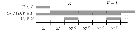
Figure 1: Schematic presentation of the potentially infinite set of clauses that is satisfiable if and only if an LTL-specification $S=(\Sigma,I,T,G)$ has a $(K,L)$-model with $K=2$ and $L=3$. The axis represents the infinite signature $\Sigma^{*}$, while the grey bars stand for individual copies of the initial, step, and goal clauses, respectively.

We have now reduced LTL satisfiability of a specification $\mathcal{S}$ to infinitely many (for every pair of $K$ and $L$) infinite propositional problems over $\Sigma^{*}$. We proceed by assigning labels to the clauses of $\mathcal{S}$ such that a labelled clause represents up to infinitely many standard clauses over $\Sigma^{*}$. Then an inference performed between labelled clauses corresponds to infinitely many inferences on the level of $\Sigma^{*}$. This is similar to the idea of “lifting” from first-order theorem proving where clauses with variables represent up to infinitely many ground instances. Here, however, we deal with the additional dimension of performing infinitely many reasoning tasks on the “ground level” in parallel, one for each pair $(K,L)$.

Definition 4

A label is a triple $(b,k,l)\in\{*,0\}\times(\{*\}\cup\mathbb{N})\times\mathbb{N}$. A labelled clause $\mathcal{C}$ is a pair $(b,k,l)\,||\,C$ consisting of a label and a standard clause over $\Sigma^{*}$.

Semantics of labels is given via a map to certain sets of time indices.

Definition 5

Let $K\in\mathbb{N}$ and $L\in\mathbb{N}^{+}$ be given. We define a set $R_{(K,L)}(b,k,l)$ of indices represented by the label $(b,k,l)$ as the set of all $t\in\mathbb{N}$ such that

1. $b\neq*\rightarrow t=0$ and

2. $k\neq*\rightarrow\exists s\in\mathbb{N}\,.\,t+k=K+s\cdot L$ and

3. $L$ divides $l$.

Now a standard clause of the form $C^{(t)}$ is said to be represented by the labelled clause $(b,k,l)\,||\,C$ in $(K,L)$ if $t\in R_{(K,L)}(b,k,l)$.

The three label components stand for three independent conditions on the time indices to which the clause relates. The first label component $b$ relates the clause to the beginning of time, and the second component relates the clause to the indices of the form $K+i\cdot L$, where the goal should be satisfied. In both cases, $*$ stands for a “don’t care” value, so if $b$ or $k$ equals $*$, the respective condition is trivially satisfied by any index. The same effect is achieved for the third condition when $l=0$, because every positive integer divides $0$.

New label values are computed from old ones using certain operations when labelled clauses interact in inferences, as will be detailed shortly. When, initially, a labelled clause set is constructed from an LTL-specification (see Definition 6 below) three particular label values are used. Further values arise as results of applying the mentioned operations, and the full generality of labels reflects an entire “closure” of the three initial values under these operations.

Definition 6

Given an LTL-specification $\mathcal{S}=(\Sigma,I,T,G)$, the initial labelled clause set $N_{\mathcal{S}}$ for $\mathcal{S}$ is defined to contain

• labelled clauses of the form $(0,*,0)\,||\,C$ for every $C\in I$,

• labelled clauses of the form $(*,*,0)\,||\,C$ for every $C\in T$, and

• labelled clauses of the form $(*,0,0)\,||\,C$ for every $C\in G$.

For any particular choice of $K$ and $L$ the standard clauses over $\Sigma^{*}$ represented by the labelled clauses from the initial labelled clause set $N_{\mathcal{S}}$ form the purely propositional problem that encodes the existence of a $(K,L)$-model of $\mathcal{S}$.

Example 1

Let us assume that a specification $\mathcal{S}$ contains a goal clause $(a\lor b)\in G$. In the initial labelled clause set $N_{S}$ this goal clause becomes $(*,0,0)\,||\,a\lor b$. If we now, for example, fix $K=2$ and $L=3$ as in Fig. 1, our labelled clause will represent all the standard clauses $(a\lor b)^{(t)}$ with $t\in R_{(2,3)}(*,0,0)=\{2,5,8,\dots\}$.

The ultimate goal of this section is to “lift” the classical resolution inference rule to labelled clauses. When two labelled clauses resolve with each other, a merge operation is applied to their labels to produce the label of the resolvent. The idea is that the labelled resolvent represents exactly those standard clauses that are resolvents of all the possible indicated resolution inferences between standard clauses represented by the labelled premises.

Definition 7 (Labelled resolution)

$$\frac{\ (b_{1},k_{1},l_{1})\,||\,A\lor C\quad(b_{2},k_{2},l_{2})\,||\,\neg A\lor D\ }{(b,k,l)\,||\,C\lor D}\enspace.$$ (1)

The two labelled clauses above the line are the inference’s premises. $A$ is an atom, $C$ and $D$ are standard clauses over $\Sigma^{*}$, and the label $(b,k,l)$ is the merge of $(b_{1},k_{1},l_{1})$ and $(b_{2},k_{2},l_{2})$ defined imperatively as follows:

• if $b_{1}=*$ then $b:=b_{2}$ else if $b_{2}=*$ then $b:=b_{1}$ else $b:=0$,

• if $k_{1}=*$ then $k:=k_{2}$ else if $k_{2}=*$ then $k:=k_{1}$ else $k:=\min(k_{1},k_{2})$,

• if $k_{1}=*$ or $k_{2}=*$ then $l:=\gcd(l_{1},l_{2})$ else $l:=\gcd(l_{1},l_{2},k_{1}-k_{2})$.

It is straightforward to verify that for every $(K,L)$ the merge operation captures the intersection of the sets of indices represented by its operands and thus the resulting label represents all the time indices where standard clauses represented by the inference’s premises interact to produce a resolvent.

Example 2

Merge of $(*,2,0)$ and $(*,5,0)$ is $(*,2,3)$; we compute the minimum of the $k$ components, and the greatest common divisor of their difference and the original $l$ components. Merge of $(*,2,3)$ and $(*,2,3)$ is $(*,2,3)$; merge is, in fact, idempotent. Merge of $(*,2,3)$ and $(*,*,0)$ is $(*,2,3)$; merge has, in fact, a neutral element $(*,*,0)$. Merge of $(*,2,3)$ and $(0,1,4)$ is $(0,1,1)$.

Not all the resolution inferences from the “ground level” of $\Sigma^{*}$ are directly visible to the labelled resolution inference (1) above. To obtain a complete correspondence, labelled resolution must, in general, be preceded by applying the following time shift operation to one of the premises, so that the atom $A$ and its matching partner $\neg A$ from the “ground level” become represented by matching counterparts in labelled clauses:

$$(*,*,l)\,||\,C \leadsto(*,*,l)\,||\,(C)^{\prime},$$ (2)

$$(*,k,l)\,||\,C \leadsto(*,k+1,l)\,||\,(C)^{\prime}.$$ (3)

Soundness of time shift is the statement that all the standard clauses represented by the right hand side of (2) and (3) are also represented by the respective left hand sides in any $(K,L)$. Note that the operation is undefined for labelled clauses with the first component $b=0$, because these only represent standard clauses fixed to the first time index.

Example 3

Let two labelled clauses $(*,0,0)\,||\,\neg p\lor q$ and $(*,0,0)\,||\,r\lor p^{\prime}$ be given. They cannot directly participate in a labelled resolution inference, although in $(K,L)=(0,1)$ there are (for every $t$) standard clauses $\neg p^{(t+1)}\lor q^{(t+1)}$ and $r^{(t)}\lor p^{(t+1)}$ represented, respectively, by the two labelled clauses, which resolve on $p^{(t+1)}$. When the first labelled clause is shifted to $(*,1,0)\,||\,\neg p^{\prime}\lor q^{\prime}$, the clauses resolve on $p^{\prime}$ and a labelled resolvent $(*,0,1)\,||\,r\lor q^{\prime}$ is obtained.

4 Elimination

By variable and clause elimination we understand the preprocessing technique described in [5] for simplifying propositional SAT problems. It consists of a combination of a controlled version of variable elimination and subsumption reduction for removing clauses, as described below. These two are alternated in a saturation loop until no further immediate improvement is possible. This section describes how the mechanism of labelled clauses can be used to adapt variable and clause elimination to the context of LTL.

Propositional variable elimination relies on exhaustive application of the resolution inference rule. Given (standard) clauses $C=p\lor C_{0}$ and $D=\neg p\lor D_{0}$, their standard resolvent $C\otimes D$ is $C_{0}\lor D_{0}$. Now, given a propositional problem in CNF consisting of a set of clauses $N$ and a variable $p$, one separates $N$ into three disjoint subsets $N=N_{p}\cup N_{\neg p}\cup N_{0}$ of clauses. The first set, $N_{p}$, is a set of clauses containing the variable $p$ positively, the clauses from $N_{\neg p}$ contain $p$ negatively, and $N_{0}$ is a set of clauses without variable $p$. A new clause set $\overline{N}$ is obtained as $(N_{p}\otimes N_{\neg p})\cup N_{0}$, where $N_{p}\otimes N_{\neg p}=\{C\otimes D\ |\ C\in N_{p},D\in N_{\neg p}\}.$ The set $\overline{N}$ no longer contains the variable $p$ and is satisfiable if and only if $N$ is.

The obtained set $\overline{N}$ may contain tautological clauses, which are redundant and should be removed. Then the sizes of $N$ and $\overline{N}$ are compared. In general, eliminating a single variable may incur a quadratic blowup. An elimination step is only considered an improvement and should be committed to when the size of $\overline{N}$ is not greater than that of $N$ (possibly up to an additive constant). It is shown in [5] that improvement eliminations occur often in practice and that they can be used to simplify the input formula considerably.

Let us now turn to eliminating variables from LTL-specifications. We know that specifications naturally correspond to sets of labelled clauses and these in turn represent propositional problems (albeit, in general, infinite ones) from which variables can be eliminated by the standard procedure described above. There is still a complication, however, because a single variable $p\in\Sigma$ from the specification corresponds to all its “instances” $p,p^{\prime},p^{(2)},\ldots$ on the “ground level” of the signature $\Sigma^{*}$. To be able to represent the result after elimination, all these instances need to be eliminated from the ground level uniformly, in one step. This seems to be a difficult task when the specification contains a clause that mentions the variable $p$ in two different time contexts, like, for example, in $\neg p\lor q\lor p^{\prime}$. In this case the individual eliminations cannot be done independently from each other and we rule the case out from further considerations.

Remark 2

There are some interesting subcases where eliminating such a variable would, in theory, be possible and would yield useful results. Consider the SNF containing $p,\,\Box(\neg p\lor p^{\prime}),\,\Box(\neg p\lor r)$, from which $p$ can be “semantically”eliminated and one obtains $\Box r$. On the other hand, eliminating $p$ from the SNF containing $p,\,\Box(\neg p\lor\neg p^{\prime}),\,\Box(p\lor p^{\prime}),\,\Box(\neg p\lor a)$ should give us a formula whose models $(W_{i})_{i\in\mathbb{N}}$ satisfy the condition $(i\bmod 2=0\Rightarrow W_{i}\models a)$, which is a property known [21] not to be expressible by an LTL formula over the single variable $a$.

Let us now, therefore, assume that we are given a set of labelled clauses $N$, perhaps an initial labelled clause set for a specification $\mathcal{S}$, and a variable $p\in\Sigma$ such that no clause in $N$ contains more than one possibly primed occurrence of $p$. We separate $N$ into $N_{p}\cup N_{\neg p}\cup N_{0}$, a subset containing $p$ positively (possibly primed), a subset containing $p$ negatively (possibly primed), and a subset not containing $p$ at all. A new set of labelled clauses $\overline{N}$ is constructed as $(N_{p}\otimes N_{\neg p})\cup N_{0}$. This time $N_{p}\otimes N_{\neg p}$ stands for the set of all the results of performing labelled resolution inference (1) on pairs of clauses from $N_{p}$ and $N_{\neg p}$, respectively, which may include shifting one of the premises in time using the rules (2) or (3).

Example 4

Let us assume that a set $N$ contains the following labelled clauses

$$(0,*,0) \,||\,p\lor q\lor r,$$ (4)

$$(0,*,0) \,||\,\neg p\lor\neg r,$$ (5)

$$(*,*,0) \,||\,r\lor\neg p^{\prime},$$ (6)

$$(*,0,0) \,||\,\neg p\lor q,$$ (7)

and these are the only labelled clauses of $N$ mentioning variable $p$. Then eliminating $p$ from $N$ means removing the above labelled clauses and replacing them by all the possible labelled resolvents over $p$. Notice that, actually,

• the tautology $(\ref{ex_cl_1})\otimes(\ref{ex_cl_2})=(0,*,0)\,||\,q\lor r\lor\neg r$ is immediately dropped,

• and $(\ref{ex_cl_1})\otimes(\ref{ex_cl_3})$ is undefined, because temporal shift does not apply to $(\ref{ex_cl_1})$.

Thus the above four clauses are replaced in $N$ by the only nontrivial resolvent $(\ref{ex_cl_1})\otimes(\ref{ex_cl_4})=(0,0,0)\,||\,q\lor r$.

To formulate soundness theorems in this section we need a satisfiability notion for labelled clauses. We extend the definition of a $(K,L)$-model, relying on the correspondence between valuations over $\Sigma^{*}$ and interpretations (see Sect. 3).

Definition 8

Let $N_{(K,L)}=\{C^{(t)}\ |\ (b,k,l)\,||\,C\in N\ \&\ t\in R_{(K,L)}(b,k,l)\}$ denote the set of standard clauses represented in $(K,L)$ by the labelled clauses from $N$. A set of labelled clauses $N$ is called $(K,L)$-satisfiable if there is a valuation $W^{*}:\Sigma^{*}\rightarrow\{0,1\}$ which (propositionally) satisfies $N_{(K,L)}$. The set $N$ is called satisfiable if it is $(K,L)$-satisfiable for some $K\in\mathbb{N}$ and $L\in\mathbb{N}^{+}$.

Soundness of variable elimination for labelled clauses now reads.

Theorem 4.1

Let $N$ and $\overline{N}=(N_{p}\otimes N_{\neg p})\cup N_{0}$ be sets of labelled clauses as described above. Then $N$ is $(K,L)$-satifiable if and only if $\overline{N}$ is.

Apart from the previously explained limitation, there is another restriction on practical variable elimination. Consider a clause set consisting of two labelled clauses $(*,*,0)\,||\,\neg x\lor p^{\prime}$ and $(*,*,0)\,||\,\neg p\lor y^{\prime}$. Eliminating $p$ with the help of labelled resolution yields the single labelled clause $(*,*,0)\,||\,\neg x\lor y^{\prime\prime}$. This could be a useful simplification in some contexts, but notice that it got us outside SNF and LTL-specifications, because $y$ now occurs doubly primed. There is, nevertheless, an advantage in knowing that such a step can be performed (has a proper meaning), because in a more complicated clause set such a resolvent with undesirable properties might turn out to be redundant (for instance, subsumed by another clause) and would subsequently be removed anyway.

This brings forward the general question of expressivity of labelled clauses. We know that only the clauses labelled by $(0,*,0),(*,*,0)$ and $(*,0,0)$, which are the labels of the initial labelled clause set, directly correspond to initial, step and goal clauses of LTL-specification, respectively. When clauses with other labels arise during elimination, the subsequent procedure for deciding satisfiability of the resulting set needs to know how to deal with them. Interestingly, according to the following theorem, we may drop several kinds of labelled clauses just after they are created without affecting satisfiability of the clause set.

Theorem 4.2

Let $N$ be a finite set of labelled clauses and let $N^{-}$ be a subset of $N$ obtained be removing all the clauses with label of the form $(b,k,l)$ such that either $(b=0$ and $k\neq*)$ or $(l\neq 0)$. Then $N^{-}$ is satisfiable if and only if $N$ is.

Proof

One implication is trivial as $N^{-}\subseteq N$. For the other, we need an auxiliary definition. We say that a label $(b,k,l)$ is relevant for a pair $(K,L)$ if $R_{(K,L)}(b,k,l)\neq\emptyset$. Now any removed clause $(b,k,l)\,||\,C$, i.e. a clause from $N\setminus N^{-}$, with $(b=0$ and $k\neq*)$ is only relevant for pairs $(K,L)$ with $K=k$, and any removed clause with $(l\neq 0)$ is only relevant for pairs $(K,L)$ with $L$ dividing $l$.

Let $N^{-}$ be $(K_{0},L_{0})$-satisfiable, i.e. some valuation $W^{*}$ satisfies $(N^{-})_{(K_{0},L_{0})}$. We may choose $K_{1}$ of the form $K_{0}+i\cdot L_{0}$ and $L_{1}$ of the form $j\cdot L_{0}$ large enough such that none of the clauses from $N\setminus N^{-}$ is relevant for $(K_{1},L_{1})$. Therefore $(N\setminus N^{-})_{(K_{1},L_{1})}=\emptyset$. Moreover, $(N^{-})_{(K_{1},L_{1})}\subseteq(N^{-})_{(K_{0},L_{0})}$ by the choice of $K_{1}$ and $L_{1}$, and so $W^{*}$ satisfies $N_{(K_{1},L_{1})}$ and thus $N$ is $(K_{1},L_{1})$-satisfiable.

Example 5

Deriving an empty labelled clause during elimination does not immediately imply that the current clause set is unsatisfiable. For instance, the label of the empty clause $(*,0,2)\,||\,\bot$ is only relevant for $(K,L)$ when $L$ divides $2$, and thus the current clause set may still be $(K,L)$-satisfiable for $L>2$.

After filtering a clause set with the help of Theorem 4.2, it will only contain clauses with the familiar labels of the initial clause set and possibly also clauses labelled by $(*,k,0)$, $k\in\mathbb{N}$. These do not pose any further expressivity complications, as they arise naturally in our calculus LPSup [18] for LTL satisfiability.

Let us now turn our focus to reductions, namely to showing how to extend subsumption to work with labels. We follow the same idea as with resolution. Any standard clause represented by the subsumed labelled clause must be subsumed by a standard clause represented by the subsuming labelled clause. Thus we say that $(b_{1},k_{1},l_{1})\,||\,C$ subsumes $(b_{2},k_{2},l_{2})\,||\,D$, if $C$ subsumes $D$ and the merge of the labels $(b_{1},k_{1},l_{1})$ and $(b_{2},k_{2},l_{2})$ is equal to $(b_{2},k_{2},l_{2})$. Similarly to resolution, the subsumption relation on labelled clauses can be made stronger if we allow the subsuming clause (but not the subsumed one) to be possibly shifted in time. For example, the clause $(*,*,0)\,||\,q$ subsumes $(*,1,0)\,||\,p\lor q^{\prime}$ in this sense. On the other hand, the clause $(*,*,0)\,||\,q^{\prime}$ cannot subsume $(*,*,0)\,||\,p\lor q$, because there is a standard clause represented by the latter, namely $(p\lor q)^{(0)}=p\lor q$, that is not subsumed by any standard clause represented by the former. Soundness of labelled clause elimination is stated as follows.

Theorem 4.3

Let $N$ and $\widetilde{N}$ be sets of labelled clauses, such that $\widetilde{N}\subseteq N$ and for every $\mathcal{D}\in N\setminus\widetilde{N}$ there exists $\mathcal{C}\in\widetilde{N}$ such that $\mathcal{C}$ subsumes $\mathcal{D}$. Then $N$ is $(K,L)$-satisfiable if and only if $\widetilde{N}$ is.

We close this section by shortly discussing the overall variable and clause elimination procedure. As already mentioned, it is advantageous to alternate variable elimination attempts with exhaustive application of subsumption and possibly other reductions. That’s because removing a subsumed clause may turn elimination of a particular variable into an improvement and, on the other hand, new clauses generated during elimination may be subject to subsumption. This holds true for the original SAT setting as it does with labels. A detailed description on how to efficiently organize this process can be found in [5].

5 Experimental evaluation

For our evaluation of the effectiveness of variable and clause elimination in LTL, we extended the preprocessing capabilities of Minisat [6] version 2.2. We kept Minisat’s main simplification loop, which efficiently combines variable elimination with subsumption and self-subsuming resolution, along with the fine-tuned heuristics for deciding which variables to eliminate and in what order. We emulated labels by extending respective clauses with extra marking literals and, to ensure correctness, we disallowed elimination of variables that occur both primed and unprimed in the input formula. Although this does not exploit the full potential of variable and clause elimination with labelled clauses as described in Sect. 4, we already obtained encouraging results with this setup.

For testing we used a set of LTL benchmarks collected by Schuppan and Darmawan [16]. The set consist of total 3723 problems from various sources (mostly previous papers on LTL satisfiability) and of various flavors (application, crafted, random), and represents the most comprehensive collection of LTL problems we are aware of. The testing proceeded in three stages. First, all the benchmarks were translated by our tool from the original format into LTL-specifications. Then we applied the Minisat-based elimination tool and obtained a set of simplified LTL-specifications. Finally, we ran two resolution-based LTL provers on both the original and simplified LTL-specifications to measure the effect of simplification on prover runtime. We choose the LTL prover LS4 [20], most likely the strongest LTL solver currently publically available, and trp++ [10], a well established temporal resolution prover by Boris Konev. Having performed the experiments on two independent implementations should allow us to draw more general conclusions about the effects of variable and clause elimination.

The experiments were performed on our servers with 3.16 GHz Xeon CPU, 16 GB RAM, and Debian 6.0. All the tools along with intermediate files and experiment logs can be found at http://www.mpi-inf.mpg.de/~suda/vce.html.

We recorded for each problem the number of variables and clauses that we were able to eliminate during the second stage. We distinguished variables from the original problem and auxiliary variables that were introduced during the transformation in stage one. In total, 39% of the variables (7% original, 32% auxiliary) and 32% of the clauses were eliminated. The numbers vary greatly over individual subsets of the benchmarks. For example, the family phltl allowed for almost no simplification: only 3% of the variables (just auxiliary), and 2% of the clauses could be removed. On the other hand, 99% of the variables (almost all of them original) and 98% of the clauses were removed on the family O1formula. While the former extreme can be explained by a concise and already almost clausal structure of the original formulas from phltl, the latter follows from the fact that most of the variables in O1formula occur in just one polarity, i.e. are pure. Eliminating a pure variable amounts to removal of all the clauses in which the variable appears.

Table 1: Performance of the two provers on original (o) and simplified (s) problems, grouped by problem subset. Number of problems solved by each prover within the time limit 300 seconds and the overall time spent during the attempts are shown. Unsolved problems contribute 300.0s, solved at least 0.1s due to the measurement technique. The times spent on the actual simplification are not included; these were observed to be negligible for most of the problems, with maximum of 0.3s for the largest instance.

subset	size		LS4			trp++
			solved	time		solved	time
acacia	71	o	71	7.	1s	71	39.	3s
		s	71	7.	1s	71	11.	3s
alaska	140	o	121	6607.	0s	9	39423.	2s
		s	139	882.	0s	12	38717.	5s
anzu	111	o	93	5754.	2s	0	33300.	0s
		s	94	5482.	2s	0	33300.	0s
forobots	39	o	39	4.	3s	39	1198.	8s
		s	39	3.	9s	39	194.	2s
rozier	2320	o	2278	13312.	9s	2063	96293.	7s
		s	2278	13270.	7s	2120	76921.	1s
schuppan	72	o	41	9332.	8s	36	11189.	8s
		s	41	9320.	9s	37	10741.	0s
trp	970	o	940	12327.	5s	364	189045.	2s
		s	934	11887.	5s	359	190138.	3s
total	3723	o	3583	47345.	8s	2582	370490.	0s
		s	3596	40854.	3s	2638	350023.	4s

The results of the third stage, in which we measured the effect of simplification on the performance of the two selected provers, are summarized in Table 1 and at the same time represented graphically in Fig. 2. We see that both LS4 and trp++ substantially benefit from the simplification, both in the number of solved instances and the overall runtime. On some subsets the effect is quite pronounced (see, e.g., LS4 on alaska or trp++ on forobots), while on others it is more modest. Only on the subset trp did the simplification result in less problems solved. What the table does not show, however, is that even among the trp problems there were some only solved in the simplified form (16 such problems for LS4 and 9 for trp++). When judging the relative number of problems gained by each prover, it should be noted that many problems come from scalable families and are mostly trivial or too difficult to solve. This leaves the “grey zone” where improvement is possible relatively small.

Figure 2: Comparing the number of problems solved, simplified and original, within a given time limit. Although the value ranges for LS4 (on the left) and trp++ (on the right) differ, both figures demonstrate better performance on the simplified problems.

To conclude, the result of our evaluation indicate that variable and clause elimination represents a useful preprocessing technique of LTL-specifications. Simplifying a clause set not only removes redundancies introduced by a previous, potentially sub-optimal normal form transformation (when auxiliary variables get eliminated), but usually reduces the input even further. This ultimately decreases the time needed to solve the problem. Further improvements are expected from an independent implementation that will harness the full potential of the mechanism of labels.

6 Discussion

We are not aware of any related work directly focusing on simplifying clause normal forms for LTL. However, some interesting connections can be drawn with the help of Remark 1 of Sect. 2, which shows that an LTL-specification can be viewed as a symbolic representation of a Büchi automaton. For instance, in the classical paper [9], an automaton accepting the models of an LTL formula $\varphi$ is constructed such that its states are identified with sets of $\varphi$’s subformulas. A closer look reveals an immediate connection between these subformulas and the variables introduced to represent them in the SNF for $\varphi$. The above paper also suggests several improvements of the basic algorithm. For instance, it is advocated that subformulas of the form $\mu_{1}\land\mu_{2}$ need not be stored, because the individual conjuncts $\mu_{1}$ and $\mu_{2}$ will be later added as well and they already imply the conjunction as a whole. We can restate this on the symbolic level as an observation that a variable introduced to represent a conjunctive subformula can always be eliminated, which is a claim easy to verify.

We believe this connection deserves further exploration, as one could possibly use it to bring some of the numerous techniques for optimizing explicit automata construction (see e.g. [14]) to the symbolic level. Note, however, that the main application of the explicit automata construction approach lies in model checking and so the resulting automaton is required to be equivalent to the original formula. On the other hand, our clausal symbolic approach is meant for satisfiability testing only and so more general satisfiability preserving transformations are allowed. An elimination of a variable from the original signature of the formula $\varphi$, or the “forgetting step” justified by Theorem 4.2 of Sect. 4, are examples of transformations that do not have a counterpart on the automata side.

While the explicit notion of a symbolic representation of a Büchi automaton via a clause normal form has received relatively little attention so far, symbolic approaches to LTL model checking and satisfiability based on Binary Decision Diagrams are well known [2]. Again, it seems possible that some optimization techniques could be shared between the two approaches. For instance, different BDD encodings recently studied by Rozier and Vardi [15], could correspond to different ways of turning a formula into an LTL-specification.

7 Conclusion

We have shown that variable and clause elimination, a practically successful preprocessing technique for propositional SAT problems, can be adapted to the setting of linear temporal logic. For that purpose we have utilized the mechanism of labelled clauses, a method for interpreting an LTL formula as finitely represented infinite sets of standard propositional clauses. The ideas were implemented and tested on a comprehensive set of benchmarks with encouraging results. In particular, variable and clause elimination has been shown to significantly improve subsequent runtime of resolution-based provers LS4 and trp++.

We would like to stress here that labelled clauses provide a general method for transferring resolution-based reasoning from SAT to LTL. It is therefore plausible that other preprocessing techniques, like, for example, the blocked clause elimination [11], can be adapted along the same lines. Exploring this possibility will be one of the directions for future work.

Appendix 0.A LTL preliminaries

The language of Linear Temporal Logic (LTL) formulas is an extension of the propositional language with temporal operators. The most commonly used are Next $\bigcirc$, Always $\Box$, Eventually $\Diamond$, Until $\mathsf{U}$, and Release $\mathsf{R}$. Formally, let $\Sigma=\{p,q,\ldots\}$ be a (finite) signature of propositional variables, then the set of LTL formulas is defined inductively as follows:

• any $p\in\Sigma$ is a formula,

• if $\varphi$ and $\psi$ are formulas, then so are $\neg\varphi$, $\varphi\land\psi$, and $\varphi\lor\psi$,

• if $\varphi$ and $\psi$ are formulas, then so are $\bigcirc\varphi$, $\Box\varphi$, $\Diamond\varphi$, $\varphi\mathsf{U}\psi$, and $\varphi\mathsf{R}\psi$.

A propositional valuation, or simply a state, is a mapping $W:\Sigma\rightarrow\{0,1\}$. An interpretation for an LTL formula is an infinite sequence of states $\mathcal{W}=(W_{i})_{i\in\mathbb{N}}$. The truth relation $\mathcal{W},i\models\varphi$ between an interpretation $\mathcal{W}$, time index $i\in\mathbb{N}$, and a formula $\varphi$ is defined recursively as follows:

$\mathcal{W},i\models p$	iff $W_{i}\models p$,
$\mathcal{W},i\models\neg\varphi$	iff not $\mathcal{W},i\models\varphi$,
$\mathcal{W},i\models\varphi\land\psi$	iff $\mathcal{W},i\models\varphi$ and $\mathcal{W},i\models\psi$,
$\mathcal{W},i\models\varphi\lor\psi$	iff $\mathcal{W},i\models\varphi$ or $\mathcal{W},i\models\psi$,
$\mathcal{W},i\models\bigcirc\varphi$	iff $\mathcal{W},i+1\models\varphi$,
$\mathcal{W},i\models\Box\varphi$	iff for every $j\geq i$, $\mathcal{W},j\models\varphi$,
$\mathcal{W},i\models\Diamond\varphi$	iff for some $j\geq i$, $\mathcal{W},j\models\varphi$,

$\mathcal{W},i\models\varphi\mathsf{U}\psi$	iff there is $j\geq i$ such that $\mathcal{W},j\models\psi$
	and $\mathcal{W},k\models\varphi$ for every $k$, $i\leq k<j$,
$\mathcal{W},i\models\varphi\mathsf{R}\psi$	iff for all $j\geq i$, $\mathcal{W},j\models\psi$ or
	there is $j\geq i$ with $\mathcal{W},j\models\varphi$ and for all $k$, $i\leq k\leq j$, $\mathcal{W},k\models\psi$.

An interpretation $\mathcal{W}$ is a model of an LTL formula $\varphi$ if $\mathcal{W},0\models\varphi$. A formula $\varphi$ is called satisfiable if it has a model, and is called valid if every interpretation is a model of $\varphi$.

Appendix 0.B Transforming LTL formulas to SNF

Formulas in SNF are conjunctions of temporal clauses, each of them assuming one of the following forms:

• an initial clause: $\bigvee_{j}k_{j}$,

• a step clause: $\Box(\bigvee_{j}k_{j}\lor\bigvee_{j}\bigcirc l_{j})$,

• an eventuality clause: $\Box(\bigvee_{j}k_{j}\lor\Diamond l)$,

where $k_{j},l_{j},$ and $l$ stand for standard literals, i.e. propositional variables or their negation.

The translation of an LTL formula $\varphi$ into an equisatisfiable SNF starts by first turning $\varphi$ into an equivalent formula that is in Negation Normal Form (NNF), meaning the negation sign only occurs in front of propositional variables in the leaves of the formula tree. This can be achieved by a standard operation that “pushes negations downwards” with the help of De Morgan’s rules and temporal equivalences like $\neg\bigcirc\varphi\equiv\bigcirc\neg\varphi$, $\neg\Box\varphi\equiv\Diamond\neg\varphi$, and $\neg(\varphi\mathsf{U}\psi)\equiv(\neg\varphi)\mathsf{R}(\neg\psi)$. Finally, multiple negations are absorbed with the help of the classical equivalence $\neg\neg\varphi\equiv\varphi$. In what follows we assume that $\varphi$ is already in NNF.

1.	$\tau[\Box(\neg x\lor l)]$	$\longrightarrow$	$\Box(\neg x\lor l)$, if $l$ is a literal,
2.	$\tau[\Box(\neg x\lor(\varphi\land\psi))]$	$\longrightarrow$	$\tau[\Box(\neg x\lor\varphi)]\land\tau[\Box(\neg x\lor\psi)],$
3.	$\tau[\Box(\neg x\lor(\varphi\lor\psi))]$	$\longrightarrow$	$\Box(\neg x\lor\mathbf{u}\lor\mathbf{v})\land$
			$\tau[\Box(\neg\mathbf{u}\lor\varphi)]\land\tau[\Box(\neg\mathbf{v}\lor\psi)],$
4.	$\tau[\Box(\neg x\lor\bigcirc\varphi)]$	$\longrightarrow$	$\Box(\neg x\lor\bigcirc\mathbf{u})\land$
			$\tau[\Box(\neg\mathbf{u}\lor\varphi)],$
5.	$\tau[\Box(\neg x\lor\Box\varphi)]$	$\longrightarrow$	$\Box(\neg x\lor\mathbf{u})\land\Box(\neg\mathbf{u}\lor\bigcirc\mathbf{u})\land$
			$\tau[\Box(\neg\mathbf{u}\lor\varphi)],$
6.	$\tau[\Box(\neg x\lor\Diamond\varphi)]$	$\longrightarrow$	$\Box(\neg x\lor\Diamond\mathbf{u})\land$
			$\tau[\Box(\neg\mathbf{u}\lor\varphi)],$
7.	$\tau[\Box(\neg x\lor(\varphi\mathsf{U}\psi)]$	$\longrightarrow$	$\Box(\neg x\lor\Diamond\mathbf{v})\land$
			$\Box(\neg x\lor\mathbf{v}\lor\mathbf{w})\land\Box(\neg\mathbf{w}\lor\mathbf{u})\land\Box(\neg\mathbf{w}\lor\bigcirc\mathbf{v}\lor\bigcirc\mathbf{w})\land$
			$\tau[\Box(\neg\mathbf{u}\lor\varphi)]\land\tau[\Box(\neg\mathbf{v}\lor\psi)],$
8.	$\tau[\Box(\neg x\lor(\varphi\mathsf{R}\psi)]$	$\longrightarrow$	$\Box(\neg x\lor\mathbf{w})\land\Box(\neg\mathbf{w}\lor\mathbf{v})\land\Box(\neg\mathbf{w}\lor\mathbf{u}\lor\bigcirc\mathbf{w})\land$
			$\tau[\Box(\neg\mathbf{u}\lor\varphi)]\land\tau[\Box(\neg\mathbf{v}\lor\psi)],$

Figure 3: The rules for SNF transformation. The freshly introduced variables are in bold.

The actual transformation is performed with the help of operator $\tau$ defined in Fig. 3, which recursively reduces any formula of the form $\Box(\neg x\lor\varphi)$ into the final SNF. During the process, new “fresh” variables are being introduced (we typeset them in bold) which serve two different purposes: They stand as names for subformulas (as in the case of the rules for, e.g., conjunction), and may also play a role of “trackers” that influence the value of other variables not just in the current state, but also in those to follow. This is how the semantics of, e.g., the Always operator $\Box$ is being encoded. The overall translation is triggered by the following rule

$$\varphi\ \ \ \longrightarrow\ \ \ \mathbf{i}\land\tau[\Box(\neg\mathbf{i}\lor\varphi)]\enspace,$$

with a fresh variable $\mathbf{i}$ that represents the whole formula.

Example 6

Here we work out an example from [8] to demonstrate the translation procedure. Assume we would like to prove the formula $(\Diamond p\land\Box(p\rightarrow\bigcirc p))\rightarrow\Diamond\Box p$. In refutational theorem proving we proceed by negating the formula and trying to show the negation to be unsatisfiable. By taking the negation into NNF (and translating away the implication symbol) we obtain

$$(\Diamond p\land\Box(\neg p\lor\bigcirc p))\land\Box\Diamond\neg p\enspace,$$

which is consequently translated into the following set of clauses:

$i$	By the initial rule.
$\Box(\neg i\lor\Diamond u_{1})$	The first conjunct by rule 6,
$\Box(\neg u_{1}\lor p)$	terminates by rule 1.
$\Box(\neg i\lor u_{2})$
$\Box(\neg u_{2}\lor\bigcirc u_{2})$	The second conjunct by rule 5,
$\Box(\neg u_{2}\lor u_{3}\lor v_{3})$	inside which there is disjunction (rule 3),
$\Box(\neg u_{3}\lor\neg p)$	the first argument is a literal (rule 1),
$\Box(\neg v_{3}\lor\bigcirc u_{4})$	the second goes by rule 4
$\Box(\neg u_{4}\lor p)$	and terminates by rule 1.
$\Box(\neg i\lor u_{5})$
$\Box(\neg u_{5}\lor\bigcirc u_{5})$	The third conjunct by rule 5,
$\Box(\neg u_{5}\lor\Diamond u_{6})$	inside which we apply rule 6,
$\Box(\neg u_{6}\lor\neg p)$	and terminate by rule 1.

Notice that transformation $\tau$ introduces more new variables than would be strictly necessary. For example, the variable $u_{6}$ just “connects” the last two clauses, which could be replaced by one equivalent eventuality clause $\Box(\neg u_{5}\lor\Diamond\neg p)$. This is a price we pay here for the simple statement of the transformation rules in Fig. 3 (no side conditions). An actual implementation would strive to detect the literal case as soon as possible, and thus, e.g., introduction of $u_{6}$ would be avoided.

Appendix 0.C Transforming general SNF to LTL-specification

The transformation of general SNF to LTL-specifications focuses on eventuality clauses. It consists in two simplification steps:

1. turning the conditional eventuality clauses into unconditional ones (of the form $\Box\Diamond l$),

2. reducing multiple (unconditional) eventuality clauses from the SNF into just one eventuality clause.

We present our modification of the simplifications first introduced in [4] that performs both steps at once.

Assume that an SNF of a formula contains $n$ (in general) conditional eventuality clauses

$$\Box(C_{i}\lor\Diamond l_{i})$$

for $i=1,\ldots,n$, where $C_{i}$ is the conditional part, i.e. a disjunction of literals. We remove these, and replace them with a single unconditional eventuality clause

$$\Box\Diamond\mathbf{m}$$ (8)

together with the following five step clauses for every $i=1,\ldots,n:$

$$\Box (C_{i}\lor l_{i}\lor\mathbf{t_{i}}),$$ (9)

$$\Box (\neg\mathbf{t_{i}}\lor\bigcirc l_{i}\lor\bigcirc\mathbf{t_{i}}),$$ (10)

$$\Box (\mathbf{s_{i}}\lor\neg\mathbf{t_{i}}\lor\bigcirc\neg\mathbf{s_{i}}),$$ (11)

$$\Box (\neg\mathbf{s_{i}}\lor\neg\mathbf{m}),$$ (12)

$$\Box (\mathbf{s_{i}}\lor\bigcirc\neg\mathbf{m}),$$ (13)

where again the bold variables are supposed to be new to the formula.

The idea behind the simplification is the following: If the condition $\neg C_{i}$ is satisfied in the current state and the respective eventuality $l_{i}$ is not satisfied in the same state we start “tracking” the eventuality with the help of the new variable $\mathbf{t_{i}}$ (clause 9). The tracking variable $\mathbf{t_{i}}$ is forced to stay true also in the future states unless the eventuality $l_{i}$ is finally satisfied (clause 10). Now let us look from the other side. The unconditional eventuality (clause 8) will infinitely often ensure that all the variables $\mathbf{s_{i}}$ are false in one state (clause 12) and were true in the previous state (clause 13). Thus in the intervals between states where $\mathbf{m}$ holds, there will always be two consecutive states where $\mathbf{s_{i}}$ changes from false to true. But this cannot happen if we are tracking that particular eventuality at that time (clause 11). To sum up, for each of the original eventualities we have a guarantee that in every interval between states where $\mathbf{m}$ holds the eventuality was either not triggered at all ($\neg C_{i}$ was false in the whole interval) or the eventuality was triggered and subsequently satisfied in that interval. Please consult [4] for a formal proof.

Example 7

Our previous example contained two conditional eventuality clauses $\Box(\neg i\lor\Diamond u_{1})$ and $\Box(\neg u_{5}\lor\Diamond u_{6})$. We may replace these by the following set of clauses to obtain an equisatisfiable problem with just one unconditional eventuality clause:

$\Box\Diamond m$,

$\Box(\neg i\lor u_{1}\lor t_{1})$,

$\Box(\neg t_{1}\lor\bigcirc u_{1}\lor\bigcirc t_{1})$,

$\Box(s_{1}\lor\neg t_{1}\lor\bigcirc\neg s_{1})$,

$\Box(\neg s_{1}\lor\neg m)$,

$\Box(s_{1}\lor\bigcirc\neg m)$,

$\Box(\neg u_{5}\lor u_{6}\lor t_{2})$,

$\Box(\neg t_{2}\lor\bigcirc u_{6}\lor\bigcirc t_{2})$,

$\Box(s_{2}\lor\neg t_{2}\lor\bigcirc\neg s_{2})$,

$\Box(\neg s_{2}\lor\neg m)$,

$\Box(s_{2}\lor\bigcirc\neg m)$.

References

- [1] A. Bolotov, M. Fisher, and C. Dixon. On the relationship between -automata and temporal logic normal forms. J. Logic Comput., 12(4):561–581, 2002.
- [2] E. M. Clarke, O. Grumberg, and K. Hamaguchi. Another look at LTL model checking. Formal Methods in System Design, 10(1):47–71, 1997.
- [3] E. M. Clarke, O. Grumberg, and D. Peled. Model checking. MIT Press, 2001.
- [4] A. Degtyarev, M. Fisher, and B. Konev. A simplified clausal resolution procedure for propositional linear-time temporal logic. In TABLEAUX ’02, volume 2381 of LNCS, pages 85–99. Springer, 2002.
- [5] N. Eén and A. Biere. Effective preprocessing in SAT through variable and clause elimination. In SAT’05, volume 3569 of LNCS, pages 61–75. Springer, 2005.
- [6] N. Eén and N. Sörensson. An extensible SAT-solver. In SAT’03, volume 2919 of LNCS, pages 502–518. Springer, 2003.
- [7] M. Fisher. A resolution method for temporal logic. In IJCAI’91, pages 99–104. Morgan Kaufmann Publishers Inc., 1991.
- [8] M. Fisher, C. Dixon, and M. Peim. Clausal temporal resolution. ACM Trans. Comput. Logic, 2:12–56, January 2001.
- [9] R. Gerth, D. Peled, M. Vardi, and P. Wolper. Simple on-the-fly automatic verification of linear temporal logic. In In Protocol Specification Testing and Verification, pages 3–18. Chapman & Hall, 1995.
- [10] U. Hustadt and B. Konev. Trp++ 2.0: A temporal resolution prover. In CADE-19, volume 2741 of LNCS, pages 274–278. Springer, 2003.
- [11] M. Järvisalo, A. Biere, and M. Heule. Blocked clause elimination. In TACAS, volume 6015 of LNCS, pages 129–144. Springer, 2010.
- [12] I. Pill, S. Semprini, R. Cavada, M. Roveri, R. Bloem, and A. Cimatti. Formal analysis of hardware requirements. DAC ’06, pages 821–826. ACM, 2006.
- [13] A. Pnueli. The temporal logic of programs. In 18th Annual Symposium on Foundations of Computer Science, pages 46–57. IEEE, 1977.
- [14] K. Rozier and M. Vardi. LTL satisfiability checking. In 14th International SPIN Workshop, volume 4595 of LNCS, pages 149–167. Springer, 2007.
- [15] K. Rozier and M. Vardi. A multi-encoding approach for LTL symbolic satisfiability checking. In FM, volume 6664 of LNCS, pages 417–431. Springer, 2011.
- [16] V. Schuppan and L. Darmawan. Evaluating LTL satisfiability solvers. In ATVA’11, volume 6996 of LNCS, pages 397–413. Springer, 2011.
- [17] A. P. Sistla and E. M. Clarke. The complexity of propositional linear temporal logics. J. ACM, 32:733–749, July 1985.
- [18] M. Suda and C. Weidenbach. Labelled superposition for PLTL. In LPAR-18, volume 7180 of LNCS, pages 391–405. Springer, 2012.
- [19] M. Suda and C. Weidenbach. Labelled superposition for PLTL. Research Report MPI-I-2012-RG1-001, Max-Planck-Institut für Informatik, Saarbrücken, 2012.
- [20] M. Suda and C. Weidenbach. A PLTL-prover based on labelled superposition with partial model guidance. In IJCAR, volume 7364 of LNCS, pages 537–543. Springer, 2012.
- [21] P. Wolper. Temporal logic can be more expressive. Information and Control, 56(1/2):72–99, 1983.