Deep Learning by Scattering

Abstract

We introduce general scattering transforms as mathematical models of deep neural networks with $\bf l^{2}$ pooling. Scattering networks iteratively apply complex valued unitary operators, and the pooling is performed by a complex modulus. An expected scattering defines a contractive representation of a high-dimensional probability distribution, which preserves its mean-square norm. We show that unsupervised learning can be casted as an optimization of the space contraction to preserve the volume occupied by unlabeled examples, at each layer of the network. Supervised learning and classification are performed with an averaged scattering, which provides scattering estimations for multiple classes.

1 Introduction

Hybrid generative and discriminative classifiers are powerful when there is a large databases of unlabeled examples and a much smaller set of labeled examples [10]. Building such classifiers requires to address two outstanding problems: estimating and representing a high dimensional probability distribution from unlabeled examples and integrating this representation in a supervised classifier.

Deep neural networks are remarkable implementations of this strategy, which has produced state-of-the-art results in many fields including image, video, music, speech and bio-medical data [3]. Most deep neural networks cascade linear operators followed by “pooling non-linearities” which aggregate multiple variables [9, 5, 6, 7, 11]. The hidden network variables are first estimated by unsupervised learning and are then updated together with the optimization of a supervised classifier from labeled examples. Multiple regularization criteria such as contraction and sparsity have been shown to play an important role in deep networks [11]. Despite the multiplicity of architectures, algorithms and results, there is currently a lack of mathematical models to understand their behavior.

This paper introduces a mathematical and algorithmic framework, to analyze the properties of high dimensional unsupervised and supervised classification problems with deep networks. It is built on a general scattering model of deep networks with $\bf l^{2}$ pooling, which iterates on contraction operators obtained as the complex modulus of unitary linear operators. It relies on many ideas developed in the deep network literature [3]. Section 2 proves that an expected scattering transform defines a converging deep network whose output defines a representation of the underlying probability distribution. Section 3 shows that such representations are optimized by adaptively contracting the space while preserving the volume where the distribution of unlabeled examples is concentrated. The optimization establishes a relation with sparsity, which explains mathematically why sparse regularizations are efficient for deep network learning [3]. Section 4 explains how scattering models can be estimated from a single realization with averaged scattering transforms, whose properties are analyzed. Given the large body of numerical experiments in the deep network literature, the paper concentrates on mathematical models, algorithms and proofs, which are currently lacking [3, 5, 7, 9].

Notation: The modulus of $z=a+ib\in{\mathbb{C}}$ is written $|z|=(|a|^{2}+|b|^{2})^{1/2}$. If $x=(x_{n})_{n\leq N}\in{\mathbb{C}}^{N}$ then we write $|x|=(|x_{n}|)_{n\leq N}\in{\mathbb{R}}^{N}$.

2 Expected Scattering

A scattering transform provides a model for feed-forward deep networks with $\bf l^{2}$ pooling [6, 7]. It iterates on linear unitary operators followed by complex modulus. Scattering transforms have initially been introduced with wavelet operators to build invariants to translations, which are stable to deformations, with applications to image and audio classifications [1, 2]. The following generalization only imposes the use of unitary operators, that we shall optimize from examples. It covers both convolutional and non-convolutional deep networks.

Let $X$ be a random vector defined in ${\mathbb{R}}^{N}$. We initialize ${X}_{0}=X$ and $N_{0}=N$. An expected scattering computes each network layer ${X}_{m+1}\in{\mathbb{R}}^{N_{m}}$ by transforming the previous layer ${X}_{m}$ with an operator $W_{m+1}$ from ${\mathbb{R}}^{N_{m}}$ in ${\mathbb{C}}^{N_{m+1}}$ such that

$$W_{m}^{*}\,W_{m}=Id~{}.$$

We typically have $N_{m+1}>N_{m}$ so $W_{m}$ is represented by a complex valued matrix whose rows are linearly dependent complex vectors. With an abuse of language, we still say that these operators are unitary. The $\bf l^{2}$ pooling is implemented with a complex modulus along each coordinate:

$${X}_{m+1}=|W_{m+1}({X}_{m}-E({X}_{m}))|~{}.$$ (1)

Let $UX=\{X_{m}\}_{m\in{\mathbb{N}}}$ be the set of all propagated layers. An expected scattering transform outputs

$$E(UX)=\{E({X}_{m})\}_{m\in{\mathbb{N}}}~{}.$$ (2)

This provides a representation of the probability distribution of $X$.

The operators $W_{m+1}$ encode the weights of the feed-forward network. Each unitary operator can be written $W_{m+1}x=\Big{\{}{\langle}x,\psi_{n}{\rangle}\Big{\}}_{n\leq N_{m+1}}$ with $\psi_{n}=\psi_{n}^{a}+i\psi_{n}^{b}\in{\mathbb{C}}^{N_{m}}$, where $\{\psi_{n}\}_{n\leq N_{m}}$ is a tight frame of ${\mathbb{R}}^{N_{m}}$. It groups pairs of random variables ${\langle}{X}_{m}-E({X}_{m}),\psi^{a}_{n}{\rangle}$ and ${\langle}{X}_{m}-E({X}_{m}),\psi^{b}_{n}{\rangle}$, whose variabilities are reduced by the contractive aggregation of the complex modulus

$$|{\langle}{X}_{m}-E({X}_{m}),\psi_{n}{\rangle}|=\Big{(}|{\langle}{X}_{m}-E({X}_{m}),\psi^{a}_{n}{\rangle}|^{2}+|{\langle}{X}_{m}-E({X}_{m}),\psi^{b}_{n}{\rangle}|^{2}\Big{)}^{1/2}~{}.$$

Ideally, $W_{m+1}$ groups pairs of non-correlated random variables having the same variance, so that it reduces the process variability without suppressing correlation information. A scattering can also pool and compute the $\bf l^{2}$ norm of $2^{k}$ variables instead of just $2$, by cascading each time $k-1$ more scattering contractions. This pooling is defined by operators $W_{m}$ which aggregates variables by pairs $(k^{\prime},k^{\prime\prime})$ with $\psi_{n}(k)=\delta_{k^{\prime}}(k)+i\delta_{k^{\prime\prime}}(k)$, where $\delta_{k^{\prime}}(k)=1$ if $k=k^{\prime}$ and $0$ otherwise, to progressively build each pool of $2^{k}$ variables.

The operator $W_{m+1}$ typically performs a rotation of the space to optimize the contraction, which is related to sparsity, as explained in the next section. Redundancy and hence increasing the space dimension is important to improve sparsity. Redundancy also prevents loosing information when calculating the modulus. With a redundancy factor $4$, one can indeed build operators $W_{m+1}$ from ${\mathbb{R}}^{N}$ to ${\mathbb{C}}^{2N}$ such that any $x$ has a stable recovery from $|W_{m+1}x|$ [4]. The following theorem proves that for any set of unitary operators, the expected scattering transform is contractive and preserves energy. The proof is in Appendix A.

Theorem 2.1.

The scattering operator is contractive

$$\|E(UX)-E(UY)\|^{2}=\sum_{m=0}^{\infty}\|E({X}_{m})-E({Y}_{m})\|^{2}\leq E(\|X-Y\|^{2})~{},$$ (3)

and preserves the mean-square norm

$$\|E(UX)\|^{2}=\sum_{m=0}^{\infty}\|E({X}_{m})\|^{2}=E(\|X\|^{2})~{}.$$ (4)

If $\|X\|$ is not bounded with probability $1$ then

$$\sum_{m=0}^{\infty}\|E({X}_{m})\|=\infty~{}$$ (5)

The theorem proof shows that the energy of network layers $E(\|{X}_{m}\|^{2})$ converges to $0$ as $m$ increases despite the fact that the dimension $N_{m}$ of these layers may increase to $\infty$. The convergence is exponential at first and then goes into a slow decay asymptotic regime, which explains why $\|E({X}_{m})\|$ is not summable. Expected scattering transforms computed with wavelet transforms operators $W_{m}$ define deep convolution networks [9], which are highly effective for a number of image and audio classification problems [1, 2]. The operator $W_{1}$ decomposes $x\in{\mathbb{R}}^{N}$ into $J$ complex wavelet signals of size $N$, so $N_{1}=JN$. The operator $W_{2}$ transforms the modulus of each of these wavelet signals into yet again $J$ wavelet signals of size $N$, so $N_{2}=J^{2}N$. The $m^{th}$ wavelet layer is thus of size $N_{m}=J^{m}N$ which grows exponentially to $\infty$ when $m$ increases. For processes which are not bounded, (5) proves that the decay of scattering coefficients is asymptotically very slow. During the first iterations $\|E({X}_{m})\|$ decays exponentially but it then slows down and decay slowly. In this slow regime, scattering coefficients characterize the tail of the probability distribution.

An expected scattering transform specifies a unique probability distribution of maximum entropy. Let us write ${U}_{m}X={X}_{m}$. Given an expected scattering transform $E(UX)=\{E(U_{m}X)\}_{m\in{\mathbb{Z}}}$, the Boltzmann theorem proves that the probability density $\tilde{p}(x)$ of maximum entropy which satisfies

$$\forall m\in{\mathbb{N}}~{}~{},~{}~{}\int_{{\mathbb{R}}^{N}}\,{U}_{m}x\,\tilde{p}(x)\,dx=E({U}_{m}X)$$ (6)

can be written

$$\tilde{p}(x)=\frac{1}{Z}\exp\left(-\sum_{m=0}^{\infty}{\langle}\lambda_{m},{U}_{m}x{\rangle}\right)~{}$$ (7)

where the $\lambda_{m}\in{\mathbb{R}}^{N_{m}}$ are the Lagrange multipliers associated to the constraints (6), and $Z$ is the normalization partition function. Complex audio textures are efficiently synthesized with such models [2, 1], by using wavelet operators $W_{m}$.

3 Unsupervised Learning by Optimizing Contractions

A scattering transform progressively squeezes the space. Heuristics are most often used to regularize unsupervised optimizations [bengio]. Because all operators are unitary, we show that optimizing this contraction amounts to minimizing the decay of scattering coefficients and leads to sparse representations. Estimators of expected scattering coefficients are given with error bounds.

Unsupervised learning considers a mixture $X$ of unknown classes $\{X^{(k)}\}_{k}$. We want to optimize each $W_{m}$ to then be able to discriminate each mixture component (class) at the supervised classification stage. To avoid confusing the scattering representations $E(UX^{(k)})$ of different classes, we would like to find operators $W_{m}$ which maximizes the average scattering distance between classes:

$$\sum_{k,l}p_{k}\,p_{l}\|E(UX^{(k)})-E(UX^{(l)})\|^{2}~{},$$ (8)

where $p_{k}$ is the probability of $X^{(k)}$ in the mixture $X$. However, unsupervised learning cannot minimize this average distance since we do not know the class labels $k$.

Following the greedy layerwise unsupervised learning strategy introduced by Hinton [5], we build the scattering transform layers one after the other, for increasing depth. We thus suppose that all operators $W_{n}$ are defined for $n\leq m$, before optimizing $W_{m+1}$. Since the average distance (8) of mixture components cannot be computed, it is replaced by a maximization of the mixture variance $E(\|X_{m+1}-E(X_{m+1})\|^{2})$. Since $W_{m+1}$ is unitary, and ${X}_{m+1}=|W_{m+1}({X}_{m}-E({X}_{m}))|$, we derive that

$$E(\|{X}_{m}-E({X}_{m})\|^{2})-E(\|{X}_{m+1}-E(X_{m+1})\|^{2})=\|E({X}_{m+1})\|^{2}~{}.$$

Given ${X}_{m}$, maximizing the variance of ${X}_{m+1}$ is equivalent to find a unitary operator $W_{m+1}$ which minimizes

$$\|E({X}_{m+1})\|^{2}=\|E(|W_{m+1}({X}_{m}-E({X}_{m}))|)\|^{2}~{}.$$ (9)

Minimizing the norm of this expected value enforces the sparsity of coefficients across realizations. It creates a deep network which filters realizations of $X$ so that their energy propagates across the network, as opposed to other signals which are not sparsified by the operators $W_{m+1}$ and will thus be attenuated much faster.

Expected scattering coefficients are estimated from $P$ independent examples $\{X_{i}\}_{i\leq P}$. A scattering transform of each $X_{i}$ is calculated by initializing $\overline{X}_{i,0}=X_{i}$. For each $m\geq 0$, given $\{\overline{X}_{i,m}\}_{i\leq P}$ we compute an estimator of $E({X}_{m})$ with an empirical average

$$\overline{\mu}_{m}=P^{-1}\sum_{i=1}^{P}\overline{X}_{i,m}~{}.$$ (10)

The scattering iteration replaces $E({X}_{m})$ by $\overline{\mu}_{m}$ in (1) which defines

$$\overline{X}_{i,m+1}=|W_{m+1}(\overline{X}_{i,m}-\overline{\mu}_{m})|~{}.$$ (11)

Section 4 generalizes this estimated scattering by introducing an averaged scattering operator. Appendix D proves the following upper bound of the mean-square estimation error.

Theorem 3.1.

$$E(\|\overline{\mu}_{m}-E({X}_{m})\|^{2})\leq P^{-1}\left(\sum_{n=0}^{m}\left(\sum_{k=n+1}^{\infty}\|E({X}_{k})\|^{2}\right)^{1/2}\right)^{2}\leq P^{-1}(m+1)^{2}E(\|X\|^{2})~{}.$$ (12)

Numerically, the first upper bound is typically of the order of $P^{-1}E(\|X\|^{2})$. The estimation error is therefore small relatively to $\|E(X_{m})\|^{2}$ if $P\gg E(\|X\|^{2})/\|E({X}_{m})\|^{2}$.

To optimize the operator $W_{m+1}x=\{{\langle}x,\psi_{n}{\rangle}\}_{n}$ we estimate (9) with a summation across examples:

$$P^{-2}\Big{\|}\sum_{i\leq P}|W_{m+1}(\overline{X}_{i,m}-\overline{\mu}_{i,m})|\Big{\|}^{2}=P^{-2}\sum_{n=1}^{N_{m+1}}\left(\sum_{i\leq P}\Big{|}{\langle}\overline{X}_{i,m}-\overline{\mu}_{i,m},\psi_{n}{\rangle}\Big{|}\right)^{2}~{}.$$ (13)

Minimization of such a convex functional under the unitary condition $W_{m+1}^{*}W_{m+1}=Id$ is a Procrustes type optimization, which admits a convex relaxation formulation as a Semi Definite Positive optimization [8]. Nearly optimal solutions can thus be computed, although the resolution of these SDP problems are numerically expensive. Stochastic gradient descent algorithms are typically used in applications [6].

Through this minimization, the complex modulus in (13) tends to define $\psi_{n}=\psi_{n}^{a}+i\psi_{n}^{b}$ which groups non-correlated random variables ${\langle}{\overline{X}}_{i,m}-\overline{\mu}_{i,m},\psi^{a}_{n}{\rangle}$ and ${\langle}{\overline{X}}_{i,m}-\overline{\mu}_{i,m},\psi^{b}_{n}{\rangle}$ with same variance. The summation over $i$ defines an $\bf l^{1}$ norm across different realizations. Minimizing this norm enforces the sparsity of this sequence. It produces few large coefficients and many small ones. The sparsity across realizations $i$ also implies a sparsity across $n$ for most realizations because the overall family of coefficients $\{|{\langle}{\overline{X}}_{i,m}-\overline{\mu}_{i,m},\psi_{n}{\rangle}|\}_{i,n}$ is sparse.

4 Averaged Scattering

We now explain how to compute hybrid generative and discriminative classifiers from scattering transforms, which integrate unsupervised learning with a supervised classification. It gives a mathematical model to explain the supervised refined training of deep neural networks, from an initial unsupervised training. Section 3 explains how to use unlabeled examples to optimize the unitary operators $W_{m}$, in order to preserve the discriminability property of the expected scattering transform. Given few labeled examples for each class $X^{(k)}$, (11) computes an estimation of $E(UX^{(k)})$ whose risk is bounded by (12). To classify a signal $x$, which is the realization of any unknown class $X^{(l)}$, we introduce an averaged scattering transform, which provides an estimator of $E(UX^{(l)})$.

An averaged scattering transform of a vector $x\in{\mathbb{R}}^{N}$ is initialized with ${\bar{x}}_{0}=x$. Each expected value is estimated by a block averaging $A_{m}$ applied to the network layer ${\bar{x}}_{m}\in{\mathbb{R}}^{N_{m}}$. It averages ${\bar{x}}_{m}$ over blocks $B_{j,m}$ of size $B_{j,m}^{\#}$, which define a partition of $\{1,...,N_{m}\}$:

$$A_{m}{\bar{x}}_{m}(n)=\sum_{j}\frac{1}{B_{j,m}^{\#}}\left(\sum_{k\in B_{j,m}}{\bar{x}}_{m}(k)\right)\,1_{n\in B_{j,m}}~{}.$$

The next layer of scattering coefficients is computed by applying the unitary operator $W_{m+1}$:

$${\bar{x}}_{m+1}=|W_{m+1}({\bar{x}}_{m}-A_{m}{\bar{x}}_{m})|=|W_{m+1}\,(Id-A_{m}){\bar{x}}_{m}|~{}.$$ (14)

The averaged scattering transform outputs the block averages of all layers ${\overline{U}}x=\{{\bar{x}}_{m}\}_{m\in{\mathbb{N}}}$:

$$A{\overline{U}}x=\{A_{m}{\bar{x}}_{m}\}_{m\in{\mathbb{N}}}~{}$$ (15)

Theorem 4.1.

The averaged scattering operator is contractive

$$\|x-y\|^{2}\geq\|A{\overline{U}}x-A{\overline{U}}y\|^{2}=\sum_{m=0}^{\infty}\|A_{m}{\bar{x}}_{m}-A_{m}{\bar{y}}_{m}\|^{2}~{}.$$ (16)

If $A_{m}$ averages over blocks of size at most $M$ then $\|{\bar{x}}_{m}\|^{2}\leq\|x\|^{2}\,(1-M^{-1})^{m}$ and

$$\|x\|^{2}=\|A{\overline{U}}x\|^{2}=\sum_{m=0}^{\infty}\|A_{m}{\bar{x}}_{m}\|^{2}~{}.$$ (17)

The unitary operators $W_{m}$ are optimized at the unsupervised stage, by maximizing a variance criterion which tends to increase the average distance between the unknown scattering vectors $E(UX^{(k)})$ of each class. At the supervised stage each $E(UX^{(k)})$ is estimated with an error bounded by Theorem 3.1. A generative classifier needs to optimize the block averages $A_{m}$ so that $A{\overline{U}}X^{(k)}=\{A_{m}{\overline{X}}^{(k)}_{m}\}_{m}$ gives an accurate estimator of $E(UX^{(k)})=\{E({X}_{m})\}_{m}$. As a result, the class of a signal $x$ can simply be estimated by

$$\hat{k}=\arg\min_{k}\|A{\overline{U}}x-E(UX^{(k)})\|~{}.$$

The error rate of such a classifier depends upon the estimation error of $E(UX^{(k)})=\{E({X}^{(k)}_{m})\}_{m\in{\mathbb{N}}}$ by $A{\overline{U}}x=\{A_{m}{\bar{x}}_{m}\}_{m\in{\mathbb{N}}}$ when $x$ is a realization of $X^{(k)}$. The following proposition computes an upper bound on this error.

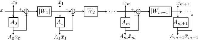
Figure 1: An averaged scattering network iteratively computes ${\bar{x}}_{m+1}=|W_{m+1}({\bar{x}}_{m}-A_{m}{\bar{x}}_{m})|$. It outputs ${\overline{U}}=\{{\bar{x}}_{m}\}_{m}$ or $A{\overline{U}}=\{A_{m}{\bar{x}}_{m}\}_{m}$ for classification.

Proposition 4.2.

$$E(\|A_{m}{\overline{X}}^{(k)}_{m}-E({X}^{(k)}_{m})\|^{2})\leq\left(\sum_{n=0}^{m}E(\|A_{n}{X}^{(k)}_{n}-E({X}^{(k)}_{n})\|^{2})^{1/2}\right)^{2}~{}.$$ (18)

The estimation error $E(\|A_{m}{\overline{X}}^{(k)}_{m}-E({X}^{(k)}_{m})\|^{2})$ is small if the averaging bias $\|A_{m}E({X}^{(k)}_{m})-E({X}^{(k)}_{m})\|^{2}$ and the variance $E(\|A_{m}{X}^{(k)}_{m}-A_{m}E({X}^{(k)}_{m})\|^{2})$ are small for all $m$ and $k$. It means that $A_{m}$ should average the largest possible groups of coefficients where $E({X}^{(k)}_{m})$ has a small variation for all $k$. Prior information is usually available to constrain the $A_{m}$. In sounds or images for example, the averaging is partly done in time or space (but not only), over intervals that must be adjusted according to the unknown local stationarity property of the ${X}^{(k)}$. This is the case for audio and image texture discrimination with wavelet scattering networks [2, 1].

Discriminative classifiers typically outperform generative classifiers, and be computed directly from ${\overline{U}}x$ as opposed to $A{\overline{U}}x$. Let us consider a binary linear classifier such as an SVM, which applies classification thresholds to ${\langle}w,A{\overline{U}}x{\rangle}$ for an optimized vector $w$. Since $A$ is a linear projector, ${\langle}w,A{\overline{U}}x{\rangle}={\langle}w^{\prime},{\overline{U}}x{\rangle}$ with $w^{\prime}=Aw$. The linear classification can thus be directly applied on ${\overline{U}}x$. Results may be improved by using $A{\overline{U}}x$ only if $A$ is a way to incorporate prior information such as local stationarity properties.

Since ${\overline{U}}x=\{{\bar{x}}_{m}\}_{m}$ is computed in (14) by iterating on $W_{m}(Id-A_{m-1})$, the supervised classifier still needs to optimize the choice of the $A_{m}$. It amounts to replacing the $W_{m}$ calculated by unsupervised learning by a new operator $W_{m}(Id-A_{m-1})$ which is optimized to minimize the classification error. Deep neural networks perform such an update of the network parameters, with a greedy layerwise supervised optimizations of the neuron weights [3]. This last step depends upon the type of discriminative classifier which is used.

5 Conclusion

A scattering transform provides a flexible model for general deep networks with $\bf l^{2}$ pooling. Imposing that linear operators are unitary preserves information and stability, and defines a network whose properties can be analyzed mathematically. It provides new models for high-dimensional probability distributions, with precise bounds on estimation errors from samples. Network parameters are optimized from unlabeled examples by adjusting the space contraction, which admits an SDP convex relaxation. Supervised classifiers are computed with an averaged scattering, which is initialized by the unsupervised estimation and refined from labeled examples.

Appendix A Proof of Theorem 2.1

Observe that $|W_{m}|$ is a contractive operator because $W_{m}$ is unitary. So

$$E(\|{X}_{m}-{Y}_{m}\|^{2}) \leq E(\|{X}_{m-1}-{Y}_{m-1}-E({X}_{m-1}-{Y}_{m-1})\|^{2})$$

$$= E(\|{X}_{m-1}-{Y}_{m-1}\|^{2})-\|E({X}_{m-1}-{Y}_{m-1})\|^{2}.$$

It results that

$$E(\|{X}_{0}-{Y}_{0}\|^{2})\geq\sum_{m=1}^{{\overline{m}}}\|E({X}_{m-1}-{Y}_{m-1})\|^{2}+E(\|{X}_{{\overline{m}}}-{Y}_{{\overline{m}}}\|^{2})~{}.$$

Letting ${\overline{m}}$ go to $\infty$ proves (3). If we set $Y=0$ then (A) is an equality so we get

$$E(\|X\|^{2})=\sum_{m=0}^{{\overline{m}}-1}\|E({X}_{m})\|^{2}+E(\|{X}_{{\overline{m}}}\|^{2})~{}.$$ (20)

To prove (4), we must show that $E(\|{X}_{{\overline{m}}}\|^{2})$ tends to $0$ when ${\overline{m}}$ goes to $\infty$. For all $M>0$,

$$E(\|{X}_{{\overline{m}}}\|^{2}) =E(\|{X}_{{\overline{m}}}\|^{2}1_{\|X\|>M})+E(\|{X}_{{\overline{m}}}\|^{2}1_{\|X\|\leq M})$$

$$\leq E(\|{X}_{{\overline{m}}}\|^{2}1_{\|X\|>M})+ME(\|{X}_{{\overline{m}}}\|1_{\|X\|\leq M}).$$ (21)

From (20), $\|E({X}_{{\overline{m}}})\|\to 0$ when ${\overline{m}}\to\infty$. From the following lemma we shall derive that $E(\|{X}_{{\overline{m}}}\|^{2})\to 0$ when ${\overline{m}}\to\infty$.

Lemma A.1.

$\lim_{{\overline{m}}\to\infty}{\bf E}(\|{X}_{{\overline{m}}}\|1_{\|X\|\leq M})=0$.

Inserting the lemma result in (21) proves that

$$\underset{{\overline{m}}}{\limsup}\,E(\|{X}_{{\overline{m}}}\|^{2})\leq\underset{{\overline{m}}}{\limsup}\,E(\|{X}_{{\overline{m}}}\|^{2}1_{\|X\|>M})$$

Observe that

$$\|{X}_{{\overline{m}}}\|^{2}\leq\|{X}_{1}\|^{2}+K~{}~{}\mbox{with}~{}~{}K=\underset{m=1}{\overset{\infty}{\sum}}\|E({X}_{m})\|^{2},$$

where $K<\infty$ because of (20). Indeed, ${X}_{m}$ has positive coordinates so

$$\|{X}_{m+1}\|^{2}=\|{X}_{m}-E({X}_{m})\|^{2}\leq\|{X}_{m}\|^{2}+\|E({X}_{m})\|^{2}$$

and hence

$$\|{X}_{{\overline{m}}}\|^{2}\leq\|{X}_{1}\|^{2}+\underset{m=1}{\overset{{\overline{m}}-1}{\sum}}\|E({X}_{m})\|^{2}\leq\|{X}_{1}\|^{2}+\underset{m=1}{\overset{\infty}{\sum}}\|E({X}_{m})\|^{2}.$$

It results that for all $M>0$

$$\underset{{\overline{m}}}{\limsup}\,E(\|{X}_{{\overline{m}}}\|^{2})\leq\underset{{\overline{m}}}{\limsup}\,\Big{(}E(\|{X}_{1}\|^{2}1_{\|X\|>M})+KE(1_{\|X\|>M})\Big{)}~{}.$$

Since ${\bf E}(\|{X}_{1}\|^{2})\leq{\bf E}(\|X\|^{2})<\infty$, the above limit tends to $0$ when $M\to\infty$ so $E(\|{X}_{{\overline{m}}}\|^{2})\to 0$.

Let us now prove Lemma A.1. Let $\epsilon$ be a positive number. Let $(E_{1},...,E_{T})$ be a partition of $\{x\in{\mathbb{R}}^{N_{0}},\|x\|_{2}\leq M\}$ in measurable non-empty sets such that, for all $t\leq T$, the diameter of $E_{t}$ is less than $\epsilon$. For all $t\leq T$, we fix $x_{t}\in E_{t}$. If $v_{1},...,v_{T}\in{\mathbb{R}}^{N_{{\overline{m}}}}$ have positive coordinates then

$$\underset{t\leq T}{\sum}\|v_{t}\|\leq\sqrt{T}\left(\underset{t\leq T}{\sum}\|v_{t}\|^{2}\right)^{1/2}\leq\sqrt{T}\Big{\|}\underset{t\leq T}{\sum}v_{t}\Big{\|}.$$

We write ${X}_{m}={U}_{m}X$. Since ${U}_{0}=Id$ and $U_{m+1}x=|W_{m}(U_{m}x-E({X}_{m}))|$, each ${U}_{m}$ is Lipschitz with constant $1$. It results that $|\|U_{m}X\|-\|U_{m}x_{t}\||\leq\|x_{t}-X\|$ and hence

$$E(\|{X}_{{\overline{m}}}\|1_{\|X\|\leq M}) =\underset{t\leq T}{\sum}E(\|{X}_{{\overline{m}}}\|1_{X\in E_{t}})=\underset{t\leq T}{\sum}E(\|U_{{\overline{m}}}X\|1_{X\in E_{t}})$$

$$\leq\underset{t\leq T}{\sum}\Big{(}E(\|U_{{\overline{m}}}x_{t}\|1_{X\in E_{t}})+E(\|x_{t}-X\|1_{X\in E_{t}})\Big{)}$$

$$=\underset{t\leq T}{\sum}\Big{(}\|E(U_{{\overline{m}}}x_{t}\,1_{X\in E_{t}})\|+E(\|x_{t}-X\|1_{X\in E_{t}})\Big{)}$$

$$\leq\underset{t\leq T}{\sum}\Big{(}\|E(U_{{\overline{m}}}X\,1_{X\in E_{t}})\|+2E(\|x_{t}-X\|1_{X\in E_{t}})\Big{)}$$

$$\leq\sqrt{T}\Big{\|}\underset{t\leq T}{\sum}E(U_{{\overline{m}}}X\,1_{X\in E_{t}})\Big{\|}+2\epsilon\underset{t\leq T}{\sum}E(1_{X\in E_{t}})$$

$$=\sqrt{T}\|E({U}_{m}X\,1_{\|X\|\leq M})\|+2\epsilon\leq\sqrt{T}\|E({X}_{{\overline{m}}})\|+2\epsilon$$

because ${X}_{{\overline{m}}}$ has positive coordinates. It results from (20) that $\lim_{{\overline{m}}\to\infty}\|E({X}_{{\overline{m}}})\|=0$ so

$$\underset{{\overline{m}}}{\limsup}\,E(\|{X}_{{\overline{m}}}\|1_{\|X\|\leq M})\leq 2\epsilon~{}.$$

Letting $\epsilon$ go to $0$ proves that $\lim_{{\overline{m}}to\infty}E(\|{X}_{{\overline{m}}}\|1_{\|X\|\leq M})=0$.

Finally, we prove (5) by contradiction: we assume that $\underset{m=0}{\overset{\infty}{\sum}}\|E({X}_{m})\|<\infty$.

$$\forall m,\quad\quad\|{X}_{m+1}\|=\|{X}_{m}-E({X}_{m})\|\geq\|{X}_{m}\|-\|E({X}_{m})\|$$

$$\Rightarrow\quad\forall{\overline{m}},\quad\quad\|{X}_{{\overline{m}}}\|\geq\max(0,\|X\|-\underset{m=0}{\overset{\infty}{\sum}}\|E({X}_{m})\|)$$

If $X$ is not bounded, this contradicts lemma A.1: for $M$ large enough,

$$\forall{\overline{m}},\quad E(\|{X}_{{\overline{m}}}\|1_{\|X\|\leq M})\geq E(1_{\|X\|\leq M}\max(0,\|X\|-\underset{m=0}{\overset{\infty}{\sum}}\|E({X}_{m})\|))>0$$

Appendix B Proof of Theorem 4.1

Since $A$ is an unitary projector and $|W_{m}|$ is contractive

$$\|{\bar{x}}_{m}-{\bar{y}}_{m}\|^{2} \leq \|{\bar{x}}_{m-1}-{\bar{y}}_{m-1}-A_{m-1}({\bar{x}}_{m-1}-{\bar{y}}_{m-1})\|^{2}$$

$$= \|{\bar{x}}_{m-1}-{\bar{y}}_{m-1}\|^{2}-\|A_{m-1}{\bar{x}}_{m-1}-A_{m-1}{\bar{y}}_{m-1})\|^{2}.$$

It results that

$$\|x-y\|^{2}\geq\sum_{m=1}^{{\overline{m}}}\|A_{m-1}({\bar{x}}_{m-1}-{\bar{y}}_{m-1})\|^{2}+\|{\bar{x}}_{{\overline{m}}}-{\bar{y}}_{{\overline{m}}}\|^{2}~{}.$$

Letting ${\overline{m}}$ go to $\infty$ proves (16). If we set $y=0$ then (B) is an equality so we get

$$\|x\|^{2}=\sum_{m=0}^{{\overline{m}}-1}\|A_{m}{\bar{x}}_{m}\|^{2}+\|{\bar{x}}_{{\overline{m}}}\|^{2}~{}.$$ (23)

Since the $A_{m}$ perform averages over blocks of size at most $M$, and ${\bar{x}}_{m}$ has positive coordinates $\|A_{m}{\bar{x}}_{m}\|^{2}\geq\|{\bar{x}}_{m}\|^{2}/M$. Since $W_{m}$ is unitary, (14) implies that

$$\|{\bar{x}}_{m+1}\|^{2}=\|{\bar{x}}_{m}-A_{m}{\bar{x}}_{m}\|^{2}=\|{\bar{x}}_{m}\|^{2}-\|A_{m}{\bar{x}}_{m}\|^{2}\leq\|{\bar{x}}_{m}\|^{2}(1-M^{-1})~{}.$$

It implies that $\|x_{\overline{m}}\|^{2}\leq\|x\|^{2}\,(1-M^{-1})^{{\overline{m}}}$. Inserting this in (23) gives (17).

Appendix C Proof of Proposition 4.2

Let us compute

$$\|A_{m}{\overline{X}}_{m}-E({X}_{m})\| = \|A_{m}{\overline{X}}_{m}-A_{m}{X}_{m}+A_{m}{X}_{m}-E({X}_{m})\|$$ (24)

$$\leq \|A_{m}({\overline{X}}_{m}-{X}_{m})\|+\|A_{m}{X}_{m}-E({X}_{m})\|$$

$$\leq \|{\overline{X}}_{m}-{X}_{m}\|+\|A_{m}{X}_{m}-E({X}_{m})\|$$

But

$$\|{\overline{X}}_{m}-{X}_{m}\| \leq \||W_{m}({\overline{X}}_{m-1}-A_{m-1}{\overline{X}}_{m-1})|-|W_{m}({X}_{m-1}-E({X}_{m-1}))|\|$$

$$\leq \||W_{m}({\overline{X}}_{m-1}-{X}_{m-1}-(A_{m-1}{\overline{X}}_{m-1}-A_{m-1}{X}_{m-1})-A_{m-1}{X}_{m-1}+E({X}_{m-1}))|\|$$

$$\leq \|W_{m}(Id-A_{m-1})({\overline{X}}_{m-1}-{X}_{m-1})\|+\|A_{m-1}{X}_{m-1})-E({X}_{m-1}))\|$$

$$\leq \|{\overline{X}}_{m-1}-{X}_{m-1}\|+\|A_{m-1}{X}_{m-1}-E({X}_{m-1})\|~{}.$$

Since ${\overline{X}}_{0}={X}_{0}$, inserting iterativey this equation in the previous equation together with (24) proves that

$$\|A_{m}{\overline{X}}_{m}-E({X}_{m})\|\leq\sum_{n=0}^{m}\|A_{n}{X}_{n}-E({X}_{n})\|~{}.$$ (25)

Since $E\left(\sum_{n}Y_{n}\right)^{2}\leq\left(\sum_{n}E(|Y_{n}|^{2})^{1/2}\right)^{2}$, we derive (18) from (25).

Appendix D Proof of Theorem 3.1

This theorem is proved by applying Proposition 4.2. To prove (12), we define an aggregated random vector $Y=\{X_{i}\}_{i\leq P}\in{\mathbb{R}}^{N\times P}$. The expected scattering tranform of $Y$ is $E({Y}_{m})=\{E({X}_{i,m})\}_{i\leq P}$ and since each $X_{i}$ has the same distribution as $X$ it results that $E({X}_{i,m})=E({X}_{m})$. Observe that ${\overline{Y}}_{m}=\{{\overline{X}}_{i,m}\}_{i\leq P}$ is an averaged scattering transform computed with

$${{\overline{Y}}}_{m+1}=|W_{m+1}({\overline{Y}}_{m}-A_{m}{\overline{Y}}_{m})|$$ (26)

where $A_{m}{\overline{Y}}_{m}$ is a vector of size $PN_{m}$ and is a concatenation $P$ vectors equal to $\bar{\mu}_{m}=P^{-1}\sum_{i=1}^{P}{\overline{X}}_{i,m}$. The vector $E({Y}_{m})$ is also of size $PN_{m}$ and is a concatenation of $P$ vectors equal to $E({X}_{m})$. Applying Proposition 18 to ${\overline{Y}}_{m}$ proves that

$$E(\|A_{m}{\overline{Y}}_{m}-E({Y}_{m})\|^{2})\leq\left(\sum_{n=0}^{m}E(\|A_{n}{Y}_{n}-E({Y}_{n})\|^{2})^{1/2}\right)^{2}~{}.$$ (27)

But $E(\|A_{m}{\overline{Y}}_{m}-E({Y}_{m})\|^{2})=PE(\|\bar{\mu}_{m}-E({X}_{m})\|^{2})$. Moreover ${Y}_{n}=\{{X}_{i,n}\}_{i\leq P}$ is a concatenation of $P$ independent random vectors of same distribution as $X_{n}$ so,

$$E(\|A_{n}{Y}_{n}-E({Y}_{n})\|^{2}=E(\|{X}_{n}-E({X}_{n})\|^{2}=\sum_{k=n}^{+\infty}E(\|{X}_{k}\|^{2})~{}.$$

Inserting these two equations in (27) together with $E(\|{X}_{k}\|^{2})\leq E(\|X\|^{2})$ proves the two inequalities of (12).

References

[1]
J. Andèn and S. Mallat, “Multiscale scattering for audio classification,” ISMIR 2011.
[2]
J. Bruna and S. Mallat, “Classification with Scattering Operators,”
CVPR 2011.
[3]
Y. Bengio, “Learning Deep Architectures for AI,” Foundations and Trends in Machine Learning, 2009.
[4]
E. J. Candès, T. Strohmer and V. Voroninski, “PhaseLift: exact and stable signal recovery from magnitude measurements via convex programming,” to appear in Comm. on Pure and Appl. Math.
[5]
G. E. Hinton, S. Osindero, M Welling, and Y. Teh, “A fast learning algorithm for deep belief nets”, Neural Computations, 18:1527-1554.
[6]
Q. Le, J. Ngiam, Z. Chen, D. Chia, P. Koh, A.Y. Ng
“Tiled Convolutional Neural Networks”, NIPS, 2010.
[7]
Q. Le, M. Ranzato, R. Monga, M. Devin, G. Corrado, K. Chen, J. Dean, A. Ng. ”Building High-Level Features Using Large Scale Unsupervised Learning” ICML 2012.
[8]
A. Nemirovski, “Sums of random symmetric matrices and quadratic optimization under orthogonality constraints”, Mathematical programming, vol. 109, no 2, 418-443, 2007.
[9]
Y. LeCun, K. Kavukvuoglu, and C. Farabet, “Convolutional Networks and Applications in Vision,” Proc. IEEE Int. Sump. Circuits and Systems 2010.
[10]
R. Raina, Y. Shen, A. Ng, A. McCallum,
“Classification with Hybrid Generative/Discriminative Models”, NIPS 2003.
[11]
S. Rifai, P. Vincent, X. Muller, X. Glorot, Y. Bengio, “Contractive Auto-Encoders: Explicit Invariance During Feature Extraction, ” ICML 2011.