Computing the Fréchet Distance with a Retractable Leash

Abstract

All known algorithms for the Fréchet distance between curves proceed in two steps: first, they construct an efficient oracle for the decision version; second, they use this oracle to find the optimum from a finite set of critical values. We present a novel approach that avoids the detour through the decision version. This gives the first quadratic time algorithm for the Fréchet distance between polygonal curves in $\mathbb{R}^{d}$ under polyhedral distance functions (e.g., $L_{1}$ and $L_{\infty}$). We also get a $(1+\varepsilon)$-approximation of the Fréchet distance under the Euclidean metric, in quadratic time for any fixed $\varepsilon>0$. For the exact Euclidean case, our framework currently yields an algorithm with running time $O(n^{2}\log^{2}n)$. However, we conjecture that it may eventually lead to a faster exact algorithm.

1 Introduction

Measuring the similarity of curves is a classic problem in computational geometry. For example, it is used for map-matching tracking data [3, 20] and moving objects analysis [8, 9]. In these applications, it is important to take the continuity of the curves into account. Therefore, the Fréchet distance and its variants are popular metrics to quantify (dis)similarity. The Fréchet distance between two curves is obtained by taking a homeomorphism between the curves that minimizes the maximum pairwise distance. It is commonly explained through the leash-metaphor: a man walks on one curve, his dog walks on the other curve. Man and dog are connected by a leash. Both can vary their speeds, but they may not walk backwards. The Fréchet distance is the length of the shortest leash so that man and dog can walk from the beginning to the end of the respective curves.

Related work.

The algorithmic study of the Fréchet distance was initiated by Alt and Godau [1]. They gave an algorithm to solve the decision version for polygonal curves in $O(n^{2})$ time, and then used parametric search to find the optimum in $O(n^{2}\log n)$ time, for two polygonal curves of complexity $n$. The method by Alt and Godau is very general and also applies to polyhedral distance functions. To avoid the need for parametric search, several randomized algorithms have been proposed that are based on the decision algorithm combined with random sampling of critical values, one running in $O(n^{2}\log^{2}n)$ time [13], the other in $O(n^{2}\log n)$ time [16]. Recently, Buchin et al. [10] showed how to solve the decision version in subquadratic time, resulting in a randomized algorithm for computing the Fréchet distance in $O(n^{2}\log^{1/2}n\log\log^{3/2}n)$ time.

In terms of the leash-metaphor, these algorithms simply give several leashes to the man and his dog to try if a walk is possible. By a clever choice of leash-lengths, one then finds the Fréchet distance efficiently. Since no substantially subquadratic algorithm for the problem is known, several faster approximation algorithms have been proposed (e.g. [2, 15]). However, these require various assumptions of the input curves; previous to our work, there was no approximation algorithm that for the general case runs faster than known exact algorithms. Recently, Bringmann [4] showed that, unless the Strong Exponential Time Hypothesis (SETH) fails, no general-case $O(n^{2-\alpha})$ algorithm can exist to approximate the Fréchet distance within a factor of $1.001$, for any $\alpha>0$. The lower bound on the approximation factor was later improved to $1.399$, even for the one-dimensional discrete case [5]. Subsequent to our work, Bringmann and Mulzer showed that a very simple greedy algorithm yields an approximation factor of $2^{O(n)}$ in linear time [5]. This leaves us with a gap between the known algorithms and lower bounds for computing and approximating the Fréchet distance.

Contribution.

We present a novel framework for computing the Fréchet distance, one that does not rely on the decision problem. Instead, we give the man a “retractable leash” that can be lengthened or shortened as required. To this end, we consider monotone paths on the distance terrain, a generalization of the free space diagram typically used for the decision problem. Similar concepts have been studied before, but without the monotonicity requirement (e.g., path planning with height restrictions on terrains [14] or the weak Fréchet distance [1]).

We present the core ideas for our approach in Section 2. The framework provides a choice of the distance function $\delta$ that is used to measure the distance between points on the curves. However, it requires an implementation of a certain data structure that depends on $\delta$. We apply our framework to polyhedral distances (Section 3), to show that under such metrics, the Fréchet distance is computable in quadratic time. To the best of our knowledge, there is no previous method for this case that is faster than the classic Alt-Godau algorithm with running time $O(mn\log n)$ [1]. Our polyhedral implementation can be used to obtain a $(1+\varepsilon)$-approximation for the Euclidean case (Section 4). This leads to an $O(mn(d+\log\frac{1}{\varepsilon}))$-time algorithm, giving the first approximation algorithm that runs faster than known exact algorithms for the general case. Moreover, as shown by Bringmann [4], our result is tight up to subpolynomial factors, assuming SETH. Finally, we apply our framework to the Euclidean distance (Section 5), to show that using this approach, we can compute the Fréchet distance in $O(mn(d+\log^{2}m+\log^{2}n))$ time for two $d$-dimensional curves of complexity $m$ and $n$. We conclude with two open problems in Section 6.

2 Framework

2.1 Preliminaries

Curves and distances.

Consider a curve $P$ in a $d$-dimensional space. We denote the vertices of $P$ by $p_{0},\dots,p_{m}$; its complexity (number of edges) is $m$. We treat a curve as a piecewise-linear function $P\colon[0,m]\rightarrow\mathbb{R}^{d}$. That is, $P(i+\lambda)=(1-\lambda)p_{i}+\lambda p_{i+1}$ holds for any integer $i\in\{0,\dots,m-1\}$ and $\lambda\in[0,1]$. Similarly, we are given a curve $Q\colon[0,n]\rightarrow\mathbb{R}^{d}$ with complexity $n$; its vertices are denoted by $q_{0},\dots,q_{n}$.

Let $\Psi$ be the set of all orientation-preserving homeomorphisms, i.e., continuous and nondecreasing functions $\psi\colon[0,m]\rightarrow[0,n]$ with $\psi(0)=0$ and $\psi(m)=n$. Then the Fréchet distance is defined as

$$d_{\text{F}}(P,Q)=\inf_{\psi\in\Psi}\max_{t\in[0,m]}\big{\{}\delta\big{(}P(t),Q(\psi(t))\big{)}\Big{\}}.$$

Here, $\delta$ may be any distance function on $\mathbb{R}^{d}$. Here, we shall consider polyhedral distance functions (Section 3) and the more typical case of the Euclidean distance function (Section 5). For our framework, we require that $\delta$ is convex. That is, the locus of all points with distance at most one to the origin forms a convex set in $\mathbb{R}^{d}$.

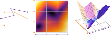
Figure 1: Illustration of a distance terrain with the Euclidean distance in $\mathbb{R}^{2}$. Left: two curves. Middle: cells as seen from above. Dark colors indicate low “height”. Right: perspective view.

Distance terrain.

Consider the joint parameter space $R=[0,m]\times[0,n]$ of $P$ and $Q$. A pair $(s,t)\in R$ corresponds to the points $P(s)$ and $Q(t)$, and the distance function $\delta$ assigns a distance $\delta(P(s),Q(t))$ to $(s,t)$. We interpret this distance as the “height” at point $(s,t)\in R$. This gives a distance terrain $T$, i.e., $T:R\rightarrow\mathbb{R}$ with $T(s,t)=\delta(P(s),Q(t))$. We partition $T$ into $mn$ cells based on the vertices of $P$ and $Q$. For integers $i\in\{0,\dots,m-1\}$ and $j\in\{0,\dots,n-1\}$, the cell $C_{i,j}$ is defined as the subset $[i,i+1]\times[j,j+1]$ of the parameter space $R$. The cells form a regular grid, where $i$ represents the column and $j$ the row of a cell. The sides of $C_{i,j}$ are the four line segments $[i,i+1]\times\{j\}$, $[i,i+1]\times\{j+1\}$, $\{i\}\times[j,j+1]$, and $\{i+1\}\times[j,j+1]$; the boundary of $C_{i,j}$ is the union of its sides. An example of two curves and their distance terrain is given in Figure 1.

A path $\pi:[0,1]\rightarrow R$ is bimonotone if it is both $x$- and $y$-monotone, i.e., every horizontal and vertical line intersects $\pi$ in at most one connected component. For $(s,t)\in R$, we let $\Pi(s,t)$ be the set of all bimonotone continuous paths from the origin to $(s,t)$. The acrophobia function $\widetilde{T}:R\rightarrow\mathbb{R}$ is defined as

$$\widetilde{T}(s,t)=\inf_{\pi\in\Pi(s,t)}\max_{\lambda\in[0,1]}T(\pi(\lambda)).$$

Intuitively, $\widetilde{T}(s,t)$ represents the lowest height that an acrophobic (and somewhat neurotic) climber needs to master in order to reach $(s,t)$ from the origin on a bimonotone path through the distance terrain $T$. A bimonotone path from $(0,0)$ to $(m,n)$ corresponds to a homeomorphism: we have $d_{\text{F}}(P,Q)=\widetilde{T}(m,n)$.

Let $x\in R$ and $\pi\in\Pi(x)$ be a bimonotone path from the origin to $x$. Let $\varepsilon\geq 0$. We call $\pi$ an $\varepsilon$-witness for $x$ if

$$\max_{\lambda\in[0,1]}T(\pi(\lambda))\leq\varepsilon.$$

For $\varepsilon=\widetilde{T}(x)$, we call $\pi$ simply a witness: $\pi$ is then an optimal path for the acrophobic climber.

Algorithm strategy.

Due to the convexity of the distance function, we need to consider only the boundaries of cells of the distance terrain. It seems natural to propagate through the terrain for any point on a cell side the minimal “height” (leash length) $\varepsilon$ required to reach that point. However, this may entail an amortized linear number of changes when moving from one cell to the next, giving a cubic-time lower bound for such an approach. We therefore do not maintain these functions explicitly. Instead, we maintain sufficient information to compute the lowest $\varepsilon$ for a side. A single pass over the terrain then finds the minimum $\varepsilon$ for reaching the other end, giving the Fréchet distance.

More specifically, we show that as we move through a row $j$ of the distance terrain from left to right, the witnesses for the minimum values of the acrophobia function on the vertical boundaries exhibit a certain monotonicity property: if a witness for the $i$-th vertical boundary enters row $j$ in column $a$, then there is a witness for the $(i+1)$-th vertical boundary that enters row $j$ in column $a$ or to the right of column $a$. Thus, if we know that the “rightmost” witness for the $i$-th vertical boundary enters row $j$ in column $a$, it suffices to consider only witnesses that enter in columns $a,a+1,\dots,i+1$. Furthermore, we can narrow down the set of candidate columns further by observing that it is enough to restrict our attention to those columns for which the minimum value of the acrophobia function on the bottom boundary is smaller than for all bottom boundaries to the right of it, up to $i+1$ (otherwise, we could find an equally good witness further to the right). Now, all we need is an efficient way to decide whether for a given candidate column, there actually exists an optimum witness for the $(i+1)$-th vertical boundary that enters row $j$ through this column. For this, we describe witness envelopes, a data structure that allows us to characterize an optimum witness that enters row $j$ in a given column. Furthermore, we show that these witness envelopes can be maintained efficiently, assuming that an appropriate data structure for dynamic upper envelopes is available. Putting everything together, and proceeding analogously for the columns of the distance terrain, we obtain a new algorithm for the Fréchet distance.

2.2 Analysis of the distance terrain

The Fréchet distance corresponds to the acrophobia function $\widetilde{T}$ on the distance terrain. To compute $\widetilde{T}(m,n)$, we show that it suffices to consider the cell boundaries. For this, we generalize the fact that cells of the free space diagram are convex [1] to the distance terrain for convex distance functions.

Lemma 2.1

Let $\varepsilon\geq 0$, and suppose that $\delta$ is a convex distance function. For every cell $C$, the set of all points $(s,t)\in C$ with $T(s,t)\leq\varepsilon$ is convex.

Proof 2.2

The cell $C$ represents the parameter space of two line segments in $\mathbb{R}^{d}$. Let $\ell_{P}(s)$ and $\ell_{Q}(t)$ be the parameterized lines spanned by these line segments. Both $\ell_{P}$ and $\ell_{Q}$ are affine maps. Consider the map $f\colon\mathbb{R}^{2}\rightarrow\mathbb{R}^{d}$ defined by $f(s,t)=\ell_{P}(s)-\ell_{Q}(t)$. Being a linear combination of affine maps, $f$ is affine. Set $D_{\varepsilon}=\{z\in\mathbb{R}^{d}\mid\delta(0,z)\leq\varepsilon\}$. Since $\delta$ is convex, $D_{\varepsilon}$ is convex. Let $E=f^{-1}(D_{\varepsilon})$. Since the affine preimage of a convex set is convex, $E$ is convex. Thus, $C\cap E$, the subset $(s,t)\in C$ with $T(s,t)\leq\varepsilon$, is convex, as it is the intersection of two convex sets.

Lemma 2.1 has two important consequences. First, it shows that it is indeed enough to focus on cell boundaries. Second, it tells us that the distance terrain along each side is unimodal, that is, it has a single local minimum.

Corollary 2.3

Let $C$ be a cell of the distance terrain, and $x_{1}$ and $x_{2}$ two points on different sides of $C$. For any $y$ on the line segment $x_{1}x_{2}$, we have $T(y)\leq\max\{T(x_{1}),T(x_{2})\}$.

Corollary 2.4

Let $C$ be a cell of the distance terrain. The restriction of $T$ to any side of $C$ is unimodal.

We denote by $L_{i,j}$ and $B_{i,j}$ the left and bottom side of the cell $C_{i,j}$ (and, by slight abuse of notation, also the restriction of $T$ to the side). The right and top side are given by $L_{i+1,j}$ and $B_{i,j+1}$. With $\widetilde{L}_{i,j}$ and $\widetilde{B}_{i,j}$ we denote the acrophobia function along the corresponding side. All these restricted functions depend on a single parameter $\alpha\in[0,1]$ in the natural way, i.e., $L_{i,j}(\alpha)=T(i,j+\alpha)$, $B_{i,j}(\alpha)=T(i+\alpha,j)$, etc. Assuming that the distance function $\delta$ is symmetric, computing values for rows and columns of $T$ is symmetric as well. Hence, we present only how to compute with rows. If $\delta$ is asymmetric, our methods still work, but some extra care needs to be taken when computing distances. In the following, we fix a row $j$, and we write $C_{i}$ as a shorthand for $C_{i,j}$, $L_{i}$ for $L_{i,j}$, etc.

Consider a vertical side $L_{i}$. We write $\widetilde{L}^{*}_{i}$ for the minimum of the acrophobia function $\widetilde{L}_{i}$ along $L_{i}$, and similarly for horizontal sides. Our goal is to compute $\widetilde{L}^{*}_{i}$ and $\widetilde{B}^{*}_{i}$ for all cell boundaries. We say that an $\varepsilon$-witness $\pi$ passes through a side $B_{i}$ if there is a $\lambda\in[0,1]$ with $\pi(\lambda)\in B_{i}$.

Lemma 2.5

Let $\varepsilon>0$, and $x$ a point on $L_{i}$. Let $\pi$ be an $\varepsilon$-witness for $x$ that passes through $B_{a}$, for some $a\in\{0,\dots,i-1\}$. Suppose there is a column $b\in\{a+1,\dots,i-1\}$ with $\widetilde{B}^{*}_{b}\leq\varepsilon$. Then there exists an $\varepsilon$-witness for $x$ that passes through $B_{b}$.

Proof 2.6

Let $y$ be a point on $B_{b}$ that achieves $\widetilde{B}^{*}_{b}$, and $\pi_{y}$ a witness for $y$. Since $\pi$ is bimonotone and passes through $B_{a}$, it must also pass through $L_{b+1}$. Let $z$ be the (lowest) intersection point of $\pi$ and $L_{b+1}$, and $\pi_{z}$ the subpath of $\pi$ from $z$ to $x$. Let $\pi^{\prime}$ be the path obtained by concatenating $\pi_{y}$, the line segment $yz$, and $\pi_{z}$. By our assumption on $\varepsilon$ and by Corollary 2.3, path $\pi^{\prime}$ is an $\varepsilon$-witness for $x$ that passes through $B_{b}$; see Figure 2.

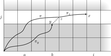
Figure 2: Suppose $x\in L_{i}$ has an $\varepsilon$-witness that passes through $B_{a}$, and $\widetilde{B}^{*}_{b}\leq\varepsilon$ for some $a<b<i$. Then, $x$ has an $\varepsilon$-witness that passes through $B_{b}$.

Lemma 2.5 implies that any point $x\in L_{i}$ has a rightmost witness $\pi$ with the property that if $\pi$ passes through the bottom side $B_{a}$, for some $a<i$, then the acrophobia function on all later bottom sides is strictly greater than the acrophobia optimum at $x$.

Corollary 2.7

Let $x$ be a point on $L_{i}$. There is a witness $\pi$ for $x$ with the following property: if $\pi$ passes through the bottom side $B_{a}$, then $\widetilde{B}^{*}_{b}>\widetilde{T}(x)$, for all $b\in\{a+1,\dots,i-1\}$.

Next, we argue that there is a witness for $\widetilde{L}^{*}_{i+1}$ that enters row $j$ at or after the bottom side used by the witness for $\widetilde{L}^{*}_{i}$. That is, the rightmost witnesses behave “monotonically” in the terrain.

Lemma 2.8

Let $\pi$ be a witness for $\widetilde{L}^{*}_{i}$ that passes through $B_{a}$, for some $a\in\{0,\dots,i-1\}$. Then $\widetilde{L}^{*}_{i+1}$ has a witness that passes through $B_{b}$, for some $b\in\{a,\dots,i\}$.

Proof 2.9

Choose $b$ maximum so that $\widetilde{L}^{*}_{i+1}$ has a witness $\pi^{\prime}$ that passes through $B_{b}$. If $b\geq a$, we are done, so assume $b<a$. Since $\pi^{\prime}$ must pass through $L_{i}$, we get $\widetilde{L}^{*}_{i+1}\geq\widetilde{L}^{*}_{i}\geq\widetilde{B}^{*}_{a}$. Lemma 2.5 now gives a witness for $\widetilde{L}^{*}_{i+1}$ that passes through $B_{a}$, despite the choice of $b$.

We now characterize $\widetilde{L}_{i}$ through a witness envelope. Fix $i\in\{1,\dots,m\}$. Suppose $\widetilde{L}^{*}_{i-1}$ has a witness that passes through $B_{a^{\prime}}$. Fix a second column $a\in\{a^{\prime},\dots,i-1\}$. We are interested in the best witness for $L_{i}$ that passes through $B_{a}$. The witness envelope is a function $\mathcal{E}_{a,i}\colon[0,1]\rightarrow\mathbb{R}$. The witnesses must pass through $B_{a}$ and $L_{i-1}$ (if $a<i-1$), and they end on $L_{i}$. Hence,

$$\mathcal{E}_{a,i}(\lambda)\geq\max\{\widetilde{B}^{*}_{a},\widetilde{L}^{*}_{i-1},L_{i}(\lambda)\}.$$

However, this is not enough to exactly characterize the best witnesses for $L_{i}$ through $B_{a}$. To this end, we introduce truncated terrain functions $\overline{L}_{b}(\lambda)=\min_{\mu\in[0,\lambda]}L_{b}(\mu)$, for $b\in\{a+1,\dots,i-1\}$. Since $L_{b}$ is unimodal, $\overline{L}_{b}$ represents the decreasing part until the minimum, remaining constant afterwards. Therefore,

$$\mathcal{E}_{a,i}(\lambda)\geq\overline{L}_{b}(\lambda),$$

for all $b=a+1,\dots,i-1$. The reason for truncating the function is as follows: to reach $L_{i}(\lambda)$, we must cross all $L_{b}$ below $y$-coordinate $j+\lambda$. If we pass $L_{b}$ below the position where the minimum is attained, the height $L_{b}$ may force a higher value for the acrophobia function. However, the increasing part of $L_{b}$ does not matter, because we could just pass $L_{b}$ closer to the minimum. This intuition is not quite accurate, since we need to account for the order of the increasing parts to ensure bimonotonicity. However, we prove below that due to the witness for $\widetilde{L}^{*}_{i-1}$ through $B_{a^{\prime}}$, this is not a problem. Thus, the witness envelope for the column interval $\{a,\dots,i\}$ in row $j$ is the upper envelope of the following functions on the interval $[0,1]$:

1. the terrain function $L_{i}(\lambda)$;

2. the constant function $\widetilde{B}^{*}_{a}$;

3. the constant function $\widetilde{L}^{*}_{i-1}$, if $a\leq i-2$; and

4. the truncated terrain functions $\overline{L}_{b}(\lambda)$, for all $b=a+1,\dots,i-1$.

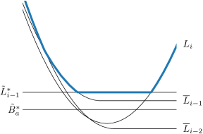
Figure 3: A witness envelope for $a=i-3$. It is the upper envelope of two constant functions, one (untruncated) terrain function, and two truncated terrain functions.

See Figure 3 for an example. We prove with the following lemma that the witness envelope exactly characterizes $\widetilde{L}_{i}$ for witnesses that pass through $B_{a}$.

Lemma 2.10

Fix a row $j$ and a two columns $a^{\prime}$, $i$ with $a^{\prime}\leq i-1$. Suppose that $\widetilde{L}^{*}_{i-1}$ has a witness $\pi_{i-1}$ that passes through $B_{a^{\prime}}$. Let $a\in\{a^{\prime},\dots,i-1\}$, $\alpha\in[0,1]$, and $\varepsilon>0$. The point $x=(i,j+\alpha)$ has an $\varepsilon$-witness that passes through $B_{a}$ if and only if $\varepsilon\geq\mathcal{E}_{a,i}(\alpha)$.

Proof 2.11

Let $\pi$ be an $\varepsilon$-witness for $x$ that passes through $B_{a}$. Then, $\varepsilon\geq\widetilde{B}^{*}_{a}$ and $\varepsilon\geq L_{i}(\alpha)$. If $a\leq i-2$, then $\pi$ must pass through $L_{i-1}$, so $\varepsilon\geq\widetilde{L}^{*}_{i-1}$. Since $\pi$ is bimonotone, it has to pass through $L_{b}$ for $a<b<i$. Let $y_{1}=(a+1,j+\alpha_{1}),y_{2}=(a+2,j+\alpha_{2}),\dots,y_{k}=(a+k,j+\alpha_{k})$ be the points of intersection, from left to right. Then, $\alpha_{1}\leq\alpha_{2}\leq\dots\leq\alpha_{k}\leq\alpha$ and $\varepsilon\geq T(y_{l})=L_{a+l}(\alpha_{i})\geq\overline{L}_{a+l}(\alpha)$, for all $l=1,\dots,k$. Hence, $\varepsilon\geq\mathcal{E}_{a,i}(\alpha)$.

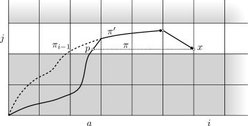
Figure 4: To construct $\pi^{\prime}$, we combine the witness for $\widetilde{B}^{*}_{a}$, the witness $\pi_{i-1}$, and the segment from $\widetilde{L}^{*}_{i-1}$ to $x$. By assumption, $\pi_{i-1}$ enters row $j$ at or to the left of $B_{a}$. If $\alpha<\alpha^{\prime}$, then $\pi^{\prime}$ is not bimonotone, and we shortcut with segment $px$ (dotted) to obtain $\pi$.

Now suppose that $\varepsilon\geq\mathcal{E}_{a,i}(\alpha)$. The conclusion is immediate for $a=i-1$. Otherwise, we have $\varepsilon\geq\widetilde{L}^{*}_{i-1}$. Let $\alpha^{\prime}$ be such that the witness $\pi_{i-1}$ for $\widetilde{L}^{*}_{i-1}$ reaches $L_{i-1}$ at point $(i-1,j+\alpha^{\prime})$. There are two cases. First, if $\alpha\geq\alpha^{\prime}$, we can find an appropriate $\varepsilon$-witness $\pi^{\prime}$ for $x$ by following the witness for $\widetilde{B}^{*}_{a}$, passing to $\pi_{i-1}$, following $\pi_{i-1}$ to $\widetilde{L}^{*}_{i-1}$, and then taking the line segment to $x$. Second, if $\alpha<\alpha^{\prime}$, we construct a curve $\pi^{\prime}$ as before. However, $\pi^{\prime}$ is not bimonotone (the last line segment goes down). This is fixed as follows: let $p$ and $x$ be the two intersection points of $\pi^{\prime}$ with the horizontal line $y=j+\alpha$. We shortcut $\pi^{\prime}$ at the line segment $px$ as illustrated in Figure 4. The resulting curve $\pi$ is bimonotone and passes through $B_{a}$. To see that $\pi$ is an $\varepsilon$-witness, it suffices to check that along the segment $px$, the distance terrain never goes above $\varepsilon$. For this, we need to consider only the intersections of $px$ with the vertical sides. Let $L_{b}$ be such a side. The function $L_{b}$ is unimodal; let $\alpha^{*}$ be the value where the minimum of $L_{b}$ is obtained. We distinguish two cases to argue that $\varepsilon\geq L_{b}(\alpha)$ and to prove the lemma:

1. $\alpha\leq\alpha^{*}$: by definition of truncated terrain functions, $L_{b}(\beta)=\overline{L}_{b}(\beta)$, for all $\beta\in[0,\alpha^{*}]$. Hence, we know that $\varepsilon\geq L_{b}(\alpha)$ holds trivially by our assumption of $\varepsilon\geq\mathcal{E}_{a,i}(\alpha)$ and the fact that $\overline{L}_{b}$ is part of the witness envelope.

2. $\alpha\geq\alpha^{*}$: by construction, the witness $\pi_{i-1}$ passes $L_{b}$ at $\alpha$ or higher. Hence, $\widetilde{L}^{*}_{i-1}\geq L_{b}(\alpha)$ holds as $L_{b}(\alpha)$ is on the increasing part of $L_{b}$. It follows that $\max\{\overline{L}_{b}(\alpha),\widetilde{L}^{*}_{i-1}\}\geq L_{b}(\alpha)$. Since $\varepsilon\geq\mathcal{E}_{a,i}(\alpha)\geq\max\{\overline{L}_{b}(\alpha),\widetilde{L}^{*}_{i-1}\}$, we have $\varepsilon\geq L_{b}(\alpha)$, as desired.

Thus, $\pi$ passes through $B_{a}$ and is an $\varepsilon$-witness for $x$.

2.3 Algorithm

We are now ready to present the algorithm. We walk through the distance terrain, row by row, in each row from left to right. When processing a cell $C_{i,j}$, we compute $\widetilde{L}^{*}_{i+1,j}$ and $\widetilde{B}^{*}_{i,j+1}$. For each row $j$, we maintain a double-ended queue (deque) $Q_{j}$ that stores a sequence of column indices. We also store a data structure $U_{j}$ that contains a set of (truncated) terrain functions on the vertical sides in row $j$. The structure $U_{j}$ supports insertion, deletion, and a minimum-point query that returns the lowest point on the upper envelope of the terrain functions. In other words, $U_{j}$ implicitly represents a witness envelope, apart from the constant functions $\widetilde{B}^{*}_{a}$ and $\widetilde{L}^{*}_{i-1}$. The implementation of $U_{j}$ depends on the distance function $\delta$: in Section 3, we describe the data structure for polyhedral distance functions, and in Section 5, we consider the Euclidean case.

Algorithm 1 $\textsc{FrechetDistance}(P,Q,\delta)$

0:  $P$ and $Q$ are polygonal curves with $m$ and $n$ edges in $\mathbb{R}^{d}$;$\delta$ is a convex distance function in $\mathbb{R}^{d}$

0:  Fréchet distance $d_{\text{F}}(P,Q)$ for $\delta$ {We show computations only within a row, column computations are analogous}

1:  $\widetilde{L}^{*}_{0,0}\leftarrow\delta(P(0),Q(0))$

2:  $\widetilde{L}^{*}_{0,j}\leftarrow\infty$ for all $j=1,\dots,n-1$

3:  For each row $j$, create empty deque $Q_{j}$ and upper envelope structure $U_{j}$

4:  for $j\leftarrow 0$ to $n-1$; $i\leftarrow 0$ to $m-1$ do

5:     Remove all values $x$ from $Q_{j}$ with $\widetilde{B}^{*}_{x,j}\geq\widetilde{B}^{*}_{i,j}$ and append $i$ to $Q_{j}$

6:     if $|Q_{j}|=1$ then

7:        Clear $U_{j}$

8:     Add $L_{i+1,j}$ to $U_{j}$

9:     Let $h$ and $h^{\prime}$ be the first and second element in $Q_{j}$

10:     $(\alpha,\varepsilon_{\alpha})\leftarrow U_{j}.\text{\sc minimumQuery}()$

11:     $\varepsilon_{\alpha}\leftarrow\max\{\varepsilon_{\alpha},\widetilde{L}^{*}_{i,j},\widetilde{B}^{*}_{h,j}\}$

12:     while $|Q_{j}|\geq 2$ and $\widetilde{B}^{*}_{h^{\prime},j}\leq\varepsilon_{\alpha}$ do

13:        Remove all $L_{x,j}$ from $U_{j}$ with $x\leq h^{\prime}$

14:        Remove the head $h$ from $Q_{j}$

15:        Let $h$ and $h^{\prime}$ be the first and second element in $Q_{j}$

16:        $(\alpha,\varepsilon_{\alpha})\leftarrow U_{j}.\text{\sc minimumQuery}()$

17:        $\varepsilon_{\alpha}\leftarrow\max\{\varepsilon_{\alpha},\widetilde{L}^{*}_{i,j},\widetilde{B}^{*}_{h,j}\}$

18:     $\widetilde{L}^{*}_{i+1,j}\leftarrow\varepsilon_{\alpha}$

19:     Update $L_{i+1,j}$ to $\overline{L}_{i+1,j}$ in $U_{j}$

20:  return  $\max\{\delta(P(m),Q(n)),\min\{\widetilde{L}^{*}_{m-1,n-1},\widetilde{B}^{*}_{m-1,n-1}\}\}$

The algorithm is given in Algorithm 1. It proceeds as follows: since all witnesses start at $(0,0)$, we initialize $C_{0,0}$ to use $(0,0)$ as its lowest point and compute the distance accordingly. The left- and bottommost sides of the distance terrain are considered unreachable.

In the body of the for-loop, we compute $\widetilde{L}^{*}_{i+1,j}$ and $\widetilde{B}^{*}_{i,j+1}$. Let us describe how to find $\widetilde{L}^{*}_{i+1,j}$. First, we remove all indices from the back of the $Q_{j}$ that have an acrophobia optimum on the bottom side that is at least $\widetilde{B}^{*}_{i,j}$, and we append $i$ to $Q_{j}$. We also add $L_{i+1,j}$ to the upper envelope $U_{j}$. Let $h$ and $h^{\prime}$ be the first two elements of $Q_{j}$. We perform a minimum query on the witness envelope, combining the result with two constants $\widetilde{L}^{*}_{i,j}$ and $\widetilde{B}^{*}_{h,j}$, in order to find the smallest $\varepsilon_{\alpha}$ for which a point on $L_{i+1,j}$ has an $\varepsilon_{\alpha}$-witness that passes through $B_{h,j}$. Note that $\widetilde{L}^{*}_{i,j}$ should be included as a constant only if $h<i$, i.e., if $|Q_{j}|\geq 2$; for simplicity, we omit this detail in the overview. If $\varepsilon_{\alpha}\geq\widetilde{B}^{*}_{h^{\prime},j}$, there is an $\varepsilon_{\alpha}$-witness for $L_{i+1,j}$ through $B_{h^{\prime},j}$, so we can repeat the process with $h^{\prime}$ (after updating $U_{j}$). If $h^{\prime}$ does not exist (i.e., $|Q_{j}|=1$) or if $\varepsilon_{\alpha}<\widetilde{B}^{*}_{h^{\prime},j}$, we stop and declare $\varepsilon_{\alpha}$ to be optimal. Finally, we update $U_{j}$ to use the truncated terrain function $\overline{L}_{i+1,j}$ instead of $L_{i+1,j}$.

We now give the invariant that holds at the beginning of each iteration of the for-loop. The invariant is stated only for a row, analogous data structures and invariants apply to the columns. A point $(\alpha,\beta)\in\mathbb{R}^{2}$ dominates a point $(\gamma,\delta)\in\mathbb{R}^{2}$ if $\alpha>\gamma$ and $\beta\leq\delta$. As before, we from now on fix a row $j$, and we omit the index $j$ from all variables.

Invariant 1

At the beginning of iteration $i+1$ in row $j$, we have computed the optima $\widetilde{L}^{*}_{1}$, $\widetilde{L}^{*}_{2}$, $\dots$, $\widetilde{L}^{*}_{i}$. Let $a$ be the column such that a rightmost witness for $\widetilde{L}^{*}_{i}$ passes through $B_{a}$. Then $Q$ stores the first coordinates of the points in the sequence $(a,\widetilde{B}^{*}_{a})$, $(a+1,\widetilde{B}^{*}_{a+1})$, $\dots$, $(i-1,\widetilde{B}^{*}_{i-1})$ that are not dominated by any other point in the sequence. In addition, $U$ stores the (truncated) terrain functions for the vertical sides in columns $a+1,\dots,i$.

Invariant 1 holds initially, so we need to prove that it is maintained in each iteration of the for-loop. This is done in the following lemma.

Lemma 2.12

Algorithm 1 maintains Invariant 1.

Proof 2.13

By the invariant, a rightmost witness for $\widetilde{L}^{*}_{i}$ passes through $B_{h_{0}}$, where $h_{0}$ is the head of $Q$ at the beginning of the iteration. Let $h^{*}$ be the column such that a rightmost witness for $\widetilde{L}^{*}_{i+1}$ passes through $B_{h^{*}}$. Then $h^{*}$ is contained in $Q$ after $i$ has been added, because by Lemma 2.8, we have $h^{*}\in\{h_{0},\dots,i\}$, and by Corollary 2.7, there can be no column index $a\in\{h^{*}+1,\dots,i\}$ that dominates $(h^{*},\widetilde{B}^{*}_{h^{*}})$.

Now let $h$ be the head of $Q$ before a minimum query on $U$, and $h^{\prime}$ the second element of $Q$. By Lemma 2.10, the minimum query gives the smallest $\varepsilon_{\alpha}$ for which there is an $\varepsilon_{\alpha}$-witness for $L_{i+1}$ that passes through $B_{h}$. If $h<h^{*}$, then $\varepsilon_{\alpha}\geq\widetilde{L}^{*}_{i+1}$ (definition of $\widetilde{L}^{*}$); $\widetilde{L}^{*}_{i+1}\geq\widetilde{B}^{*}_{h^{*}}$ (there is a witness through $B_{h^{*}}$); and $\widetilde{B}^{*}_{h^{*}}\geq\widetilde{B}^{*}_{h^{\prime}}$ (the dominance relation ensures that the $\widetilde{B}^{*}$-values for the indices in $Q$ are increasing). Thus, the while-loop in line 12 proceeds to the next iteration. If $h=h^{*}$, then by Corollary 2.7, we have $\widetilde{B}^{*}_{a}>\widetilde{B}^{*}_{h^{*}}$ for all $a\in\{h^{*}+1,\dots,i\}$, and the while-loop terminates with the correct value for $\widetilde{L}^{*}_{i}$. It is straightforward to check that Algorithm 1 maintains the data structures $Q$ and $U$ according to the invariant.

Theorem 2.14

Let $\delta$ be a convex distance function in $\mathbb{R}^{d}$. Algorithm 1 computes $d_{\text{F}}(P,Q)$ for $\delta$ in time $O(mn(T_{\text{ue}}(m,d,\delta)+T_{\text{ue}}(n,d,\delta)))$, where $T_{\text{ue}}$ represents the time to insert into, delete from, and query the upper envelope data structure.

Proof 2.15

Correctness follows from Lemma 2.12. For the running time, observe that we insert each column index only once into $Q$ and each terrain function at most twice into $U$ (once untruncated, once truncated). Hence, we can remove elements at most once or twice. This results in an amortized running time of $O(1+T_{\text{ue}}(n,d,\delta)+T_{\text{ue}}(m,d,\delta))$ for a single iteration of the for-loop. Since there are $O(mn)$ cells, this results in the claimed total execution time, assuming that $T_{\text{ue}}$ is $\Omega(1)$.

2.4 Avoiding Truncated Functions

In Algorithm 1, the envelope $U$ uses the (full) unimodal distance function only for $L_{i+1}$ and the truncated versions for the other cells. Since our algorithm relies on an efficient data structure to maintain dynamic upper envelopes of these distance functions, and since it is easier to design such a data structure if the set of possible functions to be stored is limited, we would like to avoid the need for truncating the functions. In general, this seems hard to do, but we show here that as long as the functions behave like pseudolines (i.e., each pair of functions intersects at most once, and this intersection is proper), we can actually work with the simpler set of untruncated distance functions. Since we compare only functions in the same row (or column), functions in different rows or columns may still intersect more than once. Using the full unimodal functions potentially allows for a more efficient implementation of the envelope structure.

The idea is as follows: since the terrain distance functions on the cell boundaries are unimodal, the initial (from left to right) envelopes of the truncated distance functions and the untruncated distance functions are identical. The two envelopes begin to differ only when the increasing part of an untruncated distance function “cuts off” a part of the envelope. We analyse our algorithm to understand under which circumstances this situation can occur. It turns out that in most cases, the increasing parts of the distance functions are “hidden” by the inclusion of the constant $\widetilde{L}^{*}_{i}$ in the witness envelope, except for one case, namely when the deletion of a distance function from the witness envelope exposes an increasing part of a distance function that did not previously appear on the envelope. However, we will see that this case can be detected easily, and that it can be handled by simply removing the increasing distance function from the upper envelope. The fact that the distance functions behave like pseudolines ensures that the removed function does not play any role in later queries to the witness envelope. This idea is formalized and proven below.

We modify Algorithm 1 as follows: we omit the update to $U$ in line 19, thus $U$ maintains untruncated, unimodal functions. To perform a minimum-point query, we first run the query on the upper envelope of the full unimodal functions. Let $(\alpha,\varepsilon_{\alpha})$ be the resulting minimum. If $(\alpha,\varepsilon_{\alpha})$ lies on the intersection of an increasing $L_{a}$ and a decreasing $L_{b}$ with $a<b$, we remove $L_{a}$ from $U$ and repeat the query. Otherwise, we return $\varepsilon_{\alpha}$, which is then again combined with the constants $\widetilde{L}^{*}_{i}$ and $\widetilde{B}^{*}_{h}$ as usual.

Below, we prove that this modified algorithm is indeed correct. Let $U$ be the envelope maintained by the modified algorithm (with full functions), and $\overline{U}$ the envelope of the original algorithm (with truncated functions). We let both $\overline{U}$ and $U$ include the constants $\widetilde{L}^{*}_{i}$ and $\widetilde{B}^{*}_{h}$. The envelopes $U$ and $\overline{U}$ are unimodal: they consist of a decreasing part, (possibly) followed by an increasing part. Let $D$ and $\overline{D}$ be the decreasing parts of $U$ and $\overline{U}$, up to the global minimum.

First, we make the following observation. With it, we prove that $D$ and $\overline{D}$ are identical throughout the algorithm (Invariant 2).

Lemma 2.16

Fix a terrain function $L_{a}$. Let $i\geq a$ such that $L_{a}$ is contained in $\overline{U}$ at the end of iteration $i$. Then $\widetilde{L}^{*}_{i}\geq\widetilde{L}^{*}_{a}\geq\min_{\lambda}L_{a}(\lambda)$.

Proof 2.17

By Invariant 1, there is a witness for $\widetilde{L}^{*}_{i}$ through $L_{a}$.

Invariant 2

Suppose we run the original and the modified algorithm simultaneously. Then, after each minimum query, $\overline{D}$ and $D$ are identical. Furthermore, any function that the modified algorithm deletes during a minimum query does not appear on $\overline{D}$ in any future iteration.

Proof 2.18

Initially, Invariant 2 trivially holds as the upper envelopes are empty. The envelopes $U$ and $\overline{U}$ are modified when:

1. inserting a full unimodal terrain function (line 8);

2. truncating a terrain function (line 19);

3. deleting a terrain function while updating the queue $Q$ (line 13).

We now prove that each case indeed maintains the invariant.

Case (a): The invariant tells us that $\overline{D}$ and $D$ are identical before adding a full unimodal terrain function, $L_{i+1}$. Hence, $L_{i+1}$ affects $\overline{D}$ and $D$ in the same manner (either by adding a piece or by shortening them) and Invariant 2 is maintained.

Case (b): The truncated part of $L_{i+1}$ is the increasing part and hence does not belong to $\overline{D}$. As the iteration ends, $i$ is increased by one, and $\widetilde{L}^{*}_{i+1}$ is now included in the upper envelope rather than $\widetilde{L}^{*}_{i}$. In the truncated envelope $\overline{U}$, the value of $\widetilde{L}^{*}_{i+1}$ is determined by $\overline{D}$ and the increasing part of $L_{i+1}$. Hence, the minimum remains the same when truncating $L_{i+1}$, and $\overline{D}$ is unchanged. The modified algorithm skips the truncation step, so $D$ is not changed. Again, Invariant 2 is maintained.

Case (c): After deleting a function from $U$ and $\overline{U}$, Invariant 2 may get violated. Although the invariant guarantees that all functions on $\overline{D}$ are stored by the modified algorithm, it may happen that $D$ is cut off by the increasing part of a function that is truncated in $\overline{U}$. In this case, let the minimum $p=(p_{x},p_{y})$ of $D$ be the intersection of the increasing part of $L_{a}$ and the decreasing part of $L_{b}$ in iteration $i$. There are two subcases: (c1) $b<a<i$; or (c2) $a<b<i$.

Case (c1) cannot occur: during iteration $a-1$, both the decreasing part of $L_{b}$ and the increasing part of $L_{a}$ are present in $\overline{U}$. Thus, $\widetilde{L}^{*}_{a}\geq p_{y}$, and $\widetilde{L}^{*}_{i}\geq p_{y}$, by Lemma 2.16. Therefore, $D$ cannot be a proper prefix of $\overline{D}$. In case (c2), the modified query algorithm deletes $L_{a}$ from $U$ and repeats. If we argue that $\overline{L_{a}}$ does not occur on $\overline{D}$ in any future iteration, the algorithm eventually stops with $D$ and $\overline{D}$ identical, and with Invariant 2 maintained. For this, observe that (i) $a<b$ and the decreasing part of $L_{a}$ lies below $\overline{L}_{b}$; and (ii) by Lemma 2.16, $\widetilde{L}^{*}_{i}\geq\min_{\lambda}L_{a}(\lambda)$ for any iteration $i\geq a$ in which $L_{a}$ is contained in $U$. Thus, $\overline{L}_{a}$ always lies below $\overline{D}$.

Now that we have established the desired invariant, the following theorem can be stated as a direct consequence of it.

Theorem 2.19

Let $j$ be a row of the distance terrain such that the distance functions in row $j$ intersect pairwise at most once. Then the minima computed by the modified algorithm are identical to the minima computed by the original algorithm.

3 Polyhedral distance

We consider the Fréchet distance with a convex polyhedral distance function $\delta$, i.e., the “unit sphere” of $\delta$ is a convex polytope in $\mathbb{R}^{d}$ that strictly contains the origin. For instance, the $L_{1}$ and $L_{\infty}$ distance are polyhedral with the cross-polytope and the hypercube as respective unit spheres. Throughout, we assume that $\delta$ has complexity $k$, i.e., its polytope (unit sphere) has $k$ facets. The polytope of $\delta$ is not required to be regular or symmetric, but as before, we simplify the presentation by assuming symmetry.

Intuitively, the distance $\delta(u,v)$ is the smallest scaling factor $s\geq 0$ such that $v$ lies on the polytope, centered on $u$ and scaled by a factor of $s$. We compute it as follows. Let $\mathcal{F}$ denote the facets of the polytope of $\delta$. Let $\delta_{f}(u,v)$ denote the facet distance for facet $f\in\mathcal{F}$, that is, the multiplicative factor by which the hyperplane spanned by $f$ needs to be scaled from $u$ to contain $v$. We assume that a facet $f$ is defined through the point $p_{f}$ on the hyperplane spanned by $f$ that is closest to the origin: the vector from the origin to $p_{f}$ is normal to $f$. The distance $\delta_{f}(u,v)$ is then computed as $p_{f}\cdot(v-u)/\|p_{f}\|^{2}$. This distance may be negative, but there is always at least one facet with non-negative distance. Then $\delta(u,v)=\max_{f\in\mathcal{F}}\delta_{f}(u,v)$, the maximum over all facet distances. For a general polytope, we can compute the facet distance in $O(d)$ and the distance between points in $O(kd)$ time. However, for specific polytopes, we may do better. To make this explicit in our analysis, we denote the time to compute the facet distance by $T_{\text{facet}}(\delta)$.

The distance terrain functions $L_{i,j}$ and $B_{i,j}$ are piecewise linear for a convex polyhedral distance function $\delta$. Each linear part corresponds to a facet of $\delta$. Therefore, it has at most $k$ parts. Moreover, for a fixed line segment (i.e., within the same row or column), each facet has a fixed slope: the parts for this facet are parallel. Depending on the polytope, the maximum number of parts of a single function may be less than $k$. We denote this actual maximum number of parts by $k^{\prime}$. Computing the linear parts of a distance terrain function $L_{i,j}$ or $B_{i,j}$ requires computing which facets may occur. We denote the time it takes to compute the $k^{\prime}$ relevant facets for a given boundary by $T_{\text{part}}(\delta)$.

We give three approaches. First, we use an upper envelope structure as in the Euclidean case, but exploiting that the distance functions are now piecewise linear. Second, we use a brute-force approach which is more efficient for small to moderate dimension $d$ and complexity $k$. Third, we combine these methods to deal with the case of moderately sized $d$ and $k^{\prime}$ being much smaller than $k$.

Upper envelope data structure.

As $L_{i,j}$ and $B_{i,j}$ are piecewise linear, we need a data structure that dynamically maintains the upper envelope of lines under insertions, deletions, and minimal-point queries. Note that the minimal point query now requires us to compute the actual minimal point on the upper envelope of lines (instead of parabolas). We apply the same duality transformation as in the Euclidean case and maintain a dynamic convex hull. That is, every line $\ell:y=ax+b$ on the upper envelope dualizes to a point $\ell^{*}=(a,-b)$. Any point $p=(a,b)$ dualizes to a line $p^{*}:y=ax-b$. If a point $p$ is above a line $\ell$, then the point $\ell^{*}$ is above the line $p^{*}$. Hence, the upper envelope corresponds to the dual lower convex hull. Since the minimum of the upper envelope occurs when the slopes change from negative to nonnegative, it dualizes to the line segment on the convex hull that intersects the $y$-axis. The fastest known data structure for this problem is due to Chan [12]: for $h$ lines, it has an $O(\log^{1+\tau}h)$ query and amortized update time, for any $\tau>0$.

However, in our case, we can do slightly better by using the data structure by Brodal and Jacob [7]. This data structure does not support the minimal-point query directly. However, we can make it work by observing that we must insert and delete up to $k^{\prime}$ linear functions each time; it is acceptable to run multiple queries as well.

Lemma 3.1

We can implement an upper envelope data structure structure on $h$ piecewise linear functions of complexity at most $k^{\prime}$ with an amortized update time of $O(T_{\text{part}}(\delta)+k^{\prime}T_{\text{facet}}(\delta)+k^{\prime}\log(hk^{\prime}))$ and a minimal-point query time of $O(k^{\prime}\log(hk^{\prime}))$.

Proof 3.2

First, we consider insertions and deletions. Every function is piecewise linear with at most $k^{\prime}$ parts, so there are at most $hk^{\prime}$ lines in the data structure. Hence, it takes $O(k^{\prime}\log hk^{\prime})$ amortized time to insert and delete the parts of a single function. To compute the $k^{\prime}$ relevant lines that make up the piecewise linear function, we first find the $k^{\prime}$ relevant facets of $\delta$ in $O(T_{\text{part}}(\delta))$ time. Then we compute the parameters of the corresponding lines by computing for each relevant facet $f$ the distance between $P(i)$ and $Q(j)$ and $Q(j+1)$ with respect to $f$. This takes $O(T_{\text{facet}}(\delta))$ time per facet.

For the minimal-point query, we observe that the lines with positive slope (that is, dual points with positive $x$-coordinate) are truncated at the end of each iteration. Hence, at any point during the algorithm, the dual lower hull contains at most $k^{\prime}$ points with positive $x$-coordinate. We maintain only the points with nonpositive $x$-coordinate (lines with negative slope) in the data structure. To find the line segment that intersects the $y$-axis, we perform for each current point with positive $x$-coordinate a tangent query in the convex hull structure. We maintain the tangent with the lowest intersection with the $y$-axis: this tangent gives the intersection between the $y$-axis and the actual lower hull (including the points with positive $x$-coordinate). We perform $k^{\prime}$ queries, each in $O(\log hk^{\prime})$ time; a minimal-point query takes $O(k^{\prime}\log hk^{\prime})$ time.

Brute-force approach.

A very simple data structure can often lead to good results. Here, we describe such a data structure, exploiting that in a single row, the distance function for each facet has a fixed slope. Unlike the other approaches, this method does not require computing the $k^{\prime}$ relevant facets and thus not depend on $T_{\text{part}}(\delta)$.

Lemma 3.3

After $O((m+n)k(T_{\text{facet}}(\delta)+\log k))$ total preprocessing time, we can implement the upper envelope structure with an amortized update and query time of $O(kT_{\text{facet}}(\delta))$.

Proof 3.4

During the preprocessing phase, we sort for each segment of $P$ and $Q$ the facets of $\delta$ by the corresponding slope on the witness envelope. This takes $O((m+n)k(T_{\text{facet}}(\delta)+\log k))$ total time using the straightforward algorithm.

Consider the upper envelope data structure $U_{j}$ for a row $j$ (columns are again analogous). Structure $U_{j}$ must represent a number of unimodal functions, each consisting of a number of linear parts. Each linear part corresponds to a certain facet of the polytope and has a fixed slope. For each facet $f\in\{1,\dots,k\}$ (in sorted order), structure $U_{j}$ stores a doubly linked list $F_{f}$ containing lines spanned by these linear parts. Given the fixed slope, lines in a single list $F_{f}$ do not intersect and are sorted from top to bottom. The upper envelope is fully determined only by top lines in each list $F_{f}$.

When processing a cell boundary $L_{i,j}$, we update each list $F_{l}$ in $U_{j}$: remove all lines below the line for $P(i)$ from the back of $F_{l}$, and append the line for $P(i)$. Per facet, it takes $O(T_{\text{facet}}(\delta))$ time to compute the $y$-intersection of the line and amortized $O(1)$ time for the insertion. We then go through the top lines in the $F_{l}$ in sorted order to determine the minimal value on the upper envelope in $O(k)$ time.

A hybrid approach.

We can combine the methods from Lemma 3.1 and Lemma 3.3 into a hybrid approach.

Lemma 3.5

After $O((m+n)k)$ total preprocessing time, we can implement the upper envelope structure with amortized update time $O(T_{\text{part}}(\delta)+k^{\prime}T_{\text{facet}}(\delta)+k^{\prime}\log k)$ and minimal-point query time $O(k^{\prime}\log k)$.

Proof 3.6

For each row (or column), we initialize $k$ empty lists $F_{l}$, $l=1,\dots,k$. This takes $O((m+n)k)$ total preprocessing time. The role of the $F_{l}$ is similar to Lemma 3.3, i.e., each list $F_{l}$ corresponds to a facet of the polytope. However, unlike Lemma 3.3, we do not sort the facets. Instead, we maintain the upper envelope of the top lines in each $F_{l}$, using the method from Lemma 3.1. At each cell boundary, we find the $k^{\prime}$ relevant parts and compute their parameters. The parts are inserted into the appropriate lists $F_{l}$. If a new part appears at the top of its list, we update the upper envelope structure. Since now this structure stores only $k$ lines, this takes amortized time $O(T_{\text{part}}(\delta)+k^{\prime}T_{\text{facet}}(\delta)+k^{\prime}\log k)$.

Minimal-point queries are done as before (see the proof of Lemma 3.1). Again, the structure contains only $k$ lines: a query takes $O(k^{\prime}\log k)$ time.

Plugging Lemmas 3.1, 3.3, and 3.5 into Theorem 2.14 yields the following result. The method that works best depends on the chosen polytope and on the given complexity and dimensions, that is, on the relationship between $n$, $k$, $k^{\prime}$ and $d$.

Theorem 3.7

Let $\delta$ be a convex polyhedral distance function of complexity $k$ in $\mathbb{R}^{d}$. Algorithm 1 computes the Fréchet distance under $\delta$ in

$$O\left(\min\left\{\begin{array}[]{c}mn(T_{\text{part}}(\delta)+k^{\prime}T_{\text{facet}}(\delta)+k^{\prime}\log(mnk^{\prime})),\\ (m+n)k\log k+mnkT_{\text{facet}}(\delta),\\ (m+n)k+mn(T_{\text{part}}(\delta)+k^{\prime}T_{\text{facet}}(\delta)+k^{\prime}\log k)\end{array}\right\}\right)$$

time, where $T_{\text{part}}(\delta)$ is the time needed to find the relevant parts of a distance function and $T_{\text{facet}}(\delta)$ the time needed to compute the distance between two points for a given facet of $\delta$.

Proof 3.8

The first bound follows directly from Lemma 3.1 and Theorem 2.14. For the second bound, use Lemma 3.3 and observe that $(m+n)kT_{\text{facet}}(\delta)$ is asymptotically smaller than $mnkT_{\text{facet}}(\delta)$. For the last bound, use Lemma 3.5.

For a generic polytope, we have $T_{\text{facet}}(\delta)=O(d)$, so the brute-force approach runs in $O(nk\log k+n^{2}kd)$ time. The other methods can be faster only if $k^{\prime}=o(k)$ and if we have an $o(kd)$-time method to compute the relevant facets for a distance terrain function. The hybrid method improves over the upper-envelope method if $k^{\prime}$ is much smaller than $k$. Note that there cannot be more than $\min\{k,nk^{\prime}\}$ elements in the upper envelope for the hybrid method. However, if $k>nk^{\prime}$, the upper-envelope method outperforms the hybrid method. Thus, to gain an advantage over the brute force method, a structured polytope is necessary.

Corollary 3.9

Let $\delta$ be a convex polyhedral distance function of complexity $k$ in $\mathbb{R}^{d}$. Algorithm 1 computes the Fréchet distance under $\delta$ in $O((m+n)k\log k+mnkd)$ time.

Let us now consider $L_{\infty}$. Its polytope is the hypercube; each facet is determined by a maximum coordinate. We have $k^{\prime}\leq k=2d$, and the brute-force method outperforms the other methods. However, a facet depends on only one dimension, so we compute the distance for a given facet in $T_{\text{facet}}(L_{\infty})=O(1)$ time.

Corollary 3.10

Algorithm 1 computes the Fréchet distance under the $L_{\infty}$ distance in $\mathbb{R}^{d}$ in $O((m+n)d\log d+mnd)$ time.

For $L_{1}$, the cross-polytope, there are $k=2^{d}$ facets. Structural insights help us improve upon the brute-force method. The $2^{d}$ facets of the cross-polytope are determined by the signs of the coordinates. Let $\ell=Q(j)Q(j+1)$ be the line segment and $p=P(i)$ the point defining the terrain distance $L_{i,j}$. At the breakpoints between the parts of $L_{i,j}$, one of the coordinates of $\ell-p$ changes sign. Therefore, there are at most $k^{\prime}=d+1$ parts. We find these parts efficiently by computing for each coordinate the point on $\ell-p$ where the coordinate becomes zero (if any). Sorting these values gives a representation of the relevant facets in $O(d\log d)$ time. The actual facets can then by computed in $T_{\text{part}}(L_{1})=O(d^{2})$ time. Computing the facet distance takes $T_{\text{facet}}(L_{1})=O(d)$ time, as for a general polytope. We conclude that the hybrid approach outperforms the brute-force approach. Whether the hybrid method outperforms the “pure” upper-envelope method depends on the dimension $d$.

Corollary 3.11

Algorithm 1 computes the Fréchet distance under the $L_{1}$ distance in $\mathbb{R}^{d}$ in

$$O(\min\{mn(d^{2}+d\log(mn)),(m+n)2^{d}+mnd^{2}\})$$

time.

Proof 3.12

From the arguments above and from Theorem 3.7, we know that the hybrid method runs in $O((m+n)2^{d}+mnd^{2})$ time. Similarly, the upper-envelope method runs in $O(mn(d^{2}+d\log(mnd)))$ time. Simplification of the latter gives $O(mn(d^{2}+d\log(mn)))$.

4 Approximating the Euclidean distance

We can use polyhedral distance functions to approximate the Euclidean distance. This allows us to obtain the following result.

Corollary 4.1

Algorithm 1 computes a $(1+\varepsilon)$-approximation of the Fréchet distance under the Euclidean distance in $\mathbb{R}^{d}$ in $O(mn(d+\varepsilon^{-1/2}))$ time.

Proof 4.2

A line segment $\ell$ and a point $p$ span exactly one plane in $\mathbb{R}^{d}$ (unless they are collinear, in which case we pick an arbitrary plane). On this plane, the Euclidean unit sphere $O$ is a circle; the same circle for each plane. We approximate $O$ with a $k$-regular inscribed polygon $\overline{O}$ in $\mathbb{R}^{2}$. We need to orient this polygon consistently for all points $p$, e.g., by having one side parallel to $\ell$. Simple geometry shows that for $k=O(\varepsilon^{-1/2})$, the polygon $\overline{O}$ is a $(1+\varepsilon)$-approximation to $O$. The computation is two-dimensional, but we must find the appropriate transformations, which takes $O(d)$ time per boundary. We no longer need to sort the facets of the polytope for each edge; the order is given by $\overline{O}$. This saves a logarithmic factor for the initialization of the brute-force method. This method performs best and, using Theorem 3.7, we get an execution time of $O(mn(d+\varepsilon^{-1/2})+(m+n)\varepsilon^{-1/2}\log\varepsilon^{-1/2})$. However, for $\varepsilon^{-1/2}\geq\log^{2}m+\log^{2}n$, we simply compute the exact Fréchet distance in $O(mn(d+\log^{2}m+\log^{2}n))$ time by Theorem 5.5.

Though this paper focuses on avoiding the decision-and-search paradigm, we can do better if we are willing to invoke an algorithm for the decision version of the Fréchet distance problem.

Corollary 4.3

We can calculate a $(1+\varepsilon)$-approximation of the Fréchet distance under the Euclidean distance in $O(mnd+T_{\text{dec}}(n,d)\log\varepsilon^{-1})$ time, where $T_{\text{dec}}(n,d)$ is the time needed to solve the decision problem for the Fréchet distance.

Proof 4.4

Corollary 4.1 gives a $\sqrt{2}$-approximation to the Euclidean distance in $O(mnd)$ time. Then, we go from a $\sqrt{2}$-approximation to a $(1+\varepsilon)$-approximation by binary search, using the decision algorithm.

Solving the decision version takes $T_{\text{dec}}(n,d)=O(mnd)$ time [1]. For $d=2$ and the right relation between $m$ and $n$, one can do slightly better [10, 18]: on a pointer machine, we may solve the decision version in $O(mn(\log\log n)^{3/2}/\sqrt{\log n})$, assuming $m\leq n$ and $m=\Omega(\log^{3}n)$; using a word RAM, we may solve it in $O(mn(\log\log n)^{2}/\log n)$, assuming $m\leq n$ and $m=\Omega(\log^{6}n)$.

5 Euclidean distance

Let us now consider our framework under the Euclidean distance $\delta_{\text{E}}$. The framework applies, because $\delta_{\text{E}}$ is convex (and symmetric). In fact, we use the squared Euclidean distance $\delta_{\text{E}}^{2}=\delta_{\text{E}}(x,y)^{2}$. Since squaring is a monotone function on $\mathbb{R}^{+}_{0}$, computing the Fréchet distance for the squared Euclidean distance is equivalent to the Euclidean case: if $\varepsilon=d_{\text{F}}(P,Q)$ for $\delta_{\text{E}}^{2}$, then $\sqrt{\varepsilon}=d_{\text{F}}(P,Q)$ for $\delta_{\text{E}}$. We show that the terrain functions for $\delta_{\text{E}}^{2}$ in each row and column behave like pseudolines. We consider only the vertical sides; horizontal sides are analogous.

Lemma 5.1

For $\delta=\delta_{\text{E}}^{2}$, each distance terrain function $L_{i,j}$ is part of a parabola. Any two functions $L_{i,j}$ and $L_{i^{\prime},j}$ intersect at most once.

Proof 5.2

The function $L_{i,j}$ represents the squared Euclidean distance between the point $p=P(i)$ and the line segment $\ell=Q(j)Q(j+1)$. Let $\ell^{\prime}$ be the line though $\ell$, uniformly parameterized by $\lambda\in\mathbb{R}$, i.e., $\ell^{\prime}(\lambda)=\lambda(Q(j+1)-Q(j))+Q(j)$. Let $\lambda_{p}$ be the $\lambda$ for which $\ell^{\prime}(\lambda)$ is closest to $p$. By the Pythagorean theorem, $L_{i,j}(\lambda)=\|\ell^{\prime}(\lambda)-\ell^{\prime}(\lambda_{p})\|^{2}+\|\ell^{\prime}(\lambda_{p})-p\|^{2}$. By the parametrization of $\ell^{\prime}$, we have

$$\|\ell^{\prime}(\lambda)-\ell^{\prime}(\lambda_{p})\|^{2}=\|\ell\|^{2}(\lambda-\lambda_{p})^{2}=\|\ell\|^{2}\lambda^{2}-2\|\ell\|^{2}\lambda_{p}\lambda+\|\ell\|^{2}\lambda_{p}^{2}.$$

Hence, $L_{i,j}$ is a parabolic function in $\lambda$, where the quadratic term depends only on $\ell$. For two functions in the same row, this term is the same, and thus the parabolas intersect at most once.

By Theorem 2.19 and the above lemma, we can use the modified algorithm to maintain $U_{j}$ with the full parabolas rather than truncated ones. The parabolas of a single row share the same quadratic term, so we can treat them as lines by subtracting $\|\ell\|^{2}\lambda^{2}$. In this transformed space, the constant functions $\widetilde{L}^{*}_{i,j}$ and $\widetilde{B}^{*}_{h,j}$ are now downward parabolas. This causes no problems, as these are needed only after computing the minimum on the upper envelope: we can add the term $\|\ell\|^{2}\lambda^{2}$ back to the answer before these constant functions are needed.

However, the minimum of the upper envelope of the parabolas does not necessarily correspond to the minimum of the lines. Hence, we need a “special” minimal-point query that computes the minimal point on the parabolas, using the upper envelope of the lines. The advantage of this transformation is that, by treating parabolas as lines, we may implement $U_{j}$ with a standard data structure for dynamic half-plane intersection or, dually, dynamic convex hull. The fastest such structure is due to Brodal and Jacob [7], but it does not explicitly represent the upper envelope. It is not clear if it can be modified to support our special minimal-point query. Therefore, we use the slightly slower structure by Overmars and Van Leeuwen [19], giving $O(\log^{2}h)$ time insertions and deletions, for a structure containing $h$ lines (parabolas). Most importantly, we may compute the answer to the special minimal-point query in $O(\log h)$ time.

Lemma 5.3

A minimal-point query on the upper envelope of $h$ lines can be implemented in $O(\log h)$ time.

Proof 5.4

The data structure by Overmars and Van Leeuwen maintains a concatenable queue for the upper envelope. A concatenable queue is an abstract data type providing the operations insert, delete, concatenate and split. If the queue is implemented with a red-black tree, all these operations take $O(\log h)$ time. In addition to the tree, we maintain a doubly-linked list that stores the elements in sorted order, together with cross-pointers between the corresponding nodes in the tree and in the list. The list and the cross-pointers can be updated with constant overhead. Furthermore, the list enables us to perform predecessor and successor queries in $O(1)$ time, provided that a pointer to the appropriate node is available.

The order of the points on the convex hull corresponds directly to the order of the lines, and hence of the parabolas, on their respective upper envelopes. We use the red-black tree to perform a binary search for a minimal point on the upper envelope $\mathcal{U}$ of the parabolas. We cannot decide how to proceed solely based on the parabola $p$ of a single node. However, using the predecessor and successor of $p$, we compute the local intersection pattern to guide the binary search. This is detailed below.

Let $p$ be a parabola on $\mathcal{U}$; let $l$ be the predecessor and $r$ the successor of $p$. Let $p^{*}$, $l^{*}$, and $r^{*}$ denote their respective minima. For $z\in\mathbb{R}^{2}$, let $x(z)$ be the $x$-coordinate of $z$. The parabolas $p,l,r$ pairwise intersect exactly once. Let $p_{l}=p\cap l$ and $p_{r}=p\cap r$. As $l$ and $r$ are the neighbors of $p$ on $\mathcal{U}$, we have $x(p_{l})\leq x(p_{r})$; the part of $p$ on $\mathcal{U}$ is between $p_{l}$ and $p_{r}$. We distinguish three cases (see Figure 5): (i) $x(p^{*})\leq x(p_{l})\leq x(l^{*})$; (ii) $x(p_{l})\geq x(l^{*}),x(p^{*})$; and (iii) $x(p_{l})\leq x(p^{*})$. We cannot have $x(l^{*})\leq x(p_{l})\leq x(p^{*})$: this would imply that $l$ is above $p$ right of $p_{l}$, although $l$ is the predecessor of $p$.

Figure 5: (i) The minimum is $p_{l}$; (ii) $p_{l}$ excludes the possibility that the minimum lies on or right of $p$; (iii/c) The minimum cannot be left of $p$. If the analogous case applies to $p_{r}$, the minimum of $p$ is the minimum of $\mathcal{U}$.

In case (i), $l$ is decreasing and $p$ is increasing at $p_{l}$, so $p_{l}$ is the minimum of $\mathcal{U}$. In case (ii), $p$ and the part of $\mathcal{U}$ right of $p$ do not contain the minimum, as $l$ is increasing to the left of $p_{l}$. Hence, we recurse on the left child of $p$.

In case (iii), the part of $\mathcal{U}$ left of $p_{l}$ is higher than $p$. We now consider the analogous cases for $p_{r}$: (a) $x(r^{*})\leq x(p_{r})\leq x(p^{*})$; (b) $x(p_{r})\leq x(p^{*}),x(r^{*})$; and (c) $x(p_{r})\geq x(p^{*})$. In case (a), $p_{r}$ is the minimum. In case (b), we recurse on the right child of $p$. In case (c), we get $x(p_{l})\leq x(p^{*})\leq x(p_{r})$, so $p^{*}$ is the minimum of $\mathcal{U}$.

As we can access the predecessor and successor of a node and determine the intersection pattern in constant time, a minimal-point query takes $O(\log h)$ time.

Though not necessary for our algorithm, we observe that we may actually obtain the leftmost minimal value (after including the constant functions) by performing another binary search. We obtain the following theorem.

Theorem 5.5

Algorithm 1 computes the Fréchet distance under the Euclidean distance in $\mathbb{R}^{d}$ in $O(mn(d+\log^{2}mn))$ time.

Proof 5.6

Lemma 5.1 implies that we may use the modified algorithm (Theorem 2.19). For each insertion, we have to compute the corresponding parabola, in $O(d)$ time. The data structure by Overmars and Van Leeuwen [19] allows us to implement the dynamic upper envelope of $h$ functions with $O(\log^{2}h)$-time insertions and deletions. The special minimal-point query (Lemma 5.3) takes only $O(\log h)$ time. Hence, $T_{\text{ue}}(h,d,\delta)=O(d+\log^{2}h)$ and Theorem 2.14 implies a total execution time of $O(mn(d+\log^{2}m+\log^{2}n))$. Since $\log^{2}m+\log^{2}n=\log^{2}(mn)-2\log m\log n$, the execution time can be simplified to $O(mn(d+\log^{2}(mn)))$.

Theorem 5.5 gives a slightly slower bound than known results for the Euclidean metric. However, we think that our framework has potential for a faster algorithm (see Section 6).

6 Conclusions and open problems

We introduced a new method to compute the Fréchet distance. It avoids using a decision algorithm and its consequence: a search on critical values. There is no need for parametric search. For polyhedral distance functions we gave an $O(mn)$-time algorithm. The implementation of this algorithm borders the trivial: the most advanced data structure is a doubly linked list. In addition, it can be used to compute a $(1+\varepsilon)$-approximation of the Euclidean Fréchet distance in $O(mn/\sqrt{\varepsilon})$ time or even in $O(mn\log\varepsilon^{-1})$ time, if we are willing to use a decision algorithm. For the exact Euclidean case, we obtain a slightly slower running time of $O\big{(}mn(\log^{2}m+\log^{2}n)\big{)}$. This requires dynamic convex hulls and does not really improve ease of implementation. Below, we propose two open problems for further research. For simplicity, we assume here that the two curves have the same complexity, that is, $m=n$.

Faster Euclidean distance.

We think that our current method has room for improvement; we conjecture that it is possible to extend on these ideas to obtain an $O(n^{2})$ algorithm for the Euclidean case, at least for curves in the plane. Currently we use the full power of dynamic upper envelopes, which does not seem necessary since all the information about the distance terrain functions is available in advance.

For points in the plane, we can determine the order in which the parabolas occur on the upper envelopes, in $O(n^{2})$ time for all boundaries. From the proof of Lemma 5.1, we know that the order is given by the projection of the vertices onto the line. We compute the arrangement of the lines dual to the vertices of a curve in $O(n^{2})$ time. We then determine the order of the projected points by traversing the zone of a vertical line. This takes $O(n)$ time for one row or column. Unfortunately, this alone is insufficient to obtain the quadratic time bound.

Locally correct Fréchet matchings.

A Fréchet matching is a homeomorphism $\psi\in\Psi$ such that it is a witness for the Fréchet distance, i.e., $\max_{t\in[0,n]}\delta(P(t),Q(\psi(t))=d_{\text{F}}(P,Q)$. A Fréchet matching that induces a Fréchet matching for any two matched subcurves is called a locally correct Fréchet matching [11]. It enforces a relatively “tight” matching, even if the distances are locally much smaller than the Fréchet distance of the complete curves. The algorithm by Buchin et al. [11] incurs a linear overhead on the algorithm of Alt and Godau [1], resulting in $O(n^{3}\log n)$ running time.

The discrete Fréchet distance is characterized by measuring distances only at vertices. A locally correct discrete Fréchet matching can be computed without asymptotic overhead by extending the dynamic program to compute the discrete Fréchet distance [11]. Our algorithm for the (continuous) Fréchet distance is much closer in nature to this dynamic program than to the decision-and-search paradigm of previously known methods. Therefore, we conjecture that our framework is able to avoid the linear overhead in computing a locally correct Fréchet matching. However, the information we currently propagate is insufficient: a large distance early on may “obscure” the rest of the computations, making it hard to decide which path would be locally correct.

References

- [1] H. Alt and M. Godau. Computing the Fréchet distance between two polygonal curves. Internat. J. Comput. Geom. Appl., 5(1–2):78–99, 1995.
- [2] H. Alt, C. Knauer, and C. Wenk. Matching polygonal curves with respect to the Fréchet distance. In Proc. 18th Sympos. Theoret. Aspects Comput. Sci. (STACS), pages 63–74, 2001.
- [3] S. Brakatsoulas, D. Pfoser, R. Salas, and C. Wenk. On map-matching vehicle tracking data. In Proc. 31st Int. Conf. on Very Large Data Bases (VLDB), pages 853–864, 2005.
- [4] K. Bringmann. Why walking the dog takes time: Fréchet distance has no strongly subquadratic algorithms unless SETH fails. In Proc. 55th Annu. IEEE Sympos. Found. Comput. Sci. (FOCS), pages 661–670, 2014.
- [5] K. Bringmann and W. Mulzer. Approximability of the discrete Fréchet distance. J. of Comput. Geom., 7(2):46–76, 2016.
- [6] G. S. Brodal and R. Jacob. Dynamic planar convex hull with optimal query time. In Proc. 7th Scandinavian Workshop Algorithm Theory (SWAT), pages 57–70, 2000.
- [7] G. S. Brodal and R. Jacob. Dynamic planar convex hull. In Proc. 43rd Annu. IEEE Sympos. Found. Comput. Sci. (FOCS), pages 617–626, 2002.
- [8] K. Buchin, M. Buchin, and J. Gudmundsson. Constrained free space diagrams: a tool for trajectory analysis. Int. J. of GIS, 24(7):1101–1125, 2010.
- [9] K. Buchin, M. Buchin, J. Gudmundsson, M. Löffler, and J. Luo. Detecting commuting patterns by clustering subtrajectories. Internat. J. Comput. Geom. Appl., 21(3):253–282, 2011.
- [10] K. Buchin, M. Buchin, W. Meulemans, and W. Mulzer. Four Soviets walk the dog – with an application to Alt’s conjecture. In Proc. 25th Annu. ACM-SIAM Sympos. Discrete Algorithms (SODA), pages 1399–1413, 2014.
- [11] K. Buchin, M. Buchin, W. Meulemans, and B. Speckmann. Locally correct Fréchet matchings. In Proc. 20th Annu. European Sympos. Algorithms (ESA), pages 229–240, 2012.
- [12] T. M. Chan. Three problems about dynamic convex hulls. Internat. J. Comput. Geom. Appl., 22(4):341–364, 2012.
- [13] A. F. Cook and C. Wenk. Geodesic Fréchet distance inside a simple polygon. ACM Transactions on Algorithms, 7(1):Art. 9, 2010.
- [14] M. de Berg and M. J. van Kreveld. Trekking in the Alps Without Freezing or Getting Tired. Algorithmica, 18(3):306–323, 1997.
- [15] A. Driemel, S. Har-Peled, and C. Wenk. Approximating the Fréchet distance for realistic curves in near linear time. Discrete Comput. Geom., 48(1):94–127, 2012.
- [16] S. Har-Peled and B. Raichel. The Fréchet distance revisited and extended. ACM Transactions on Algorithms, 10(1):3, 2014.
- [17] H. Kaplan, R. E. Tarjan, and K. Tsioutsiouliklis. Faster kinetic heaps and their use in broadcast scheduling. In Proc. 12th Annu. ACM-SIAM Sympos. Discrete Algorithms (SODA), pages 836–844, 2001.
- [18] W. Meulemans. Similarity Measures and Algorithms for Cartographic Schematization. PhD thesis, Eindhoven University of Technology, 2014.
- [19] M. H. Overmars and J. van Leeuwen. Maintenance of configurations in the plane. J. Comput. System Sci., 23(2):166–204, 1981.
- [20] C. Wenk, R. Salas, and D. Pfoser. Addressing the need for map-matching speed: Localizing global curve-matching algorithms. In Proc. 18th Int. Conf. on Sci. and Stat. Database Management (SSDBM), pages 379–388, 2006.