The real photon structure functions in massive parton model in NLO

We investigate the one-gluon-exchange ($\alpha\alpha_{s}$) corrections to the real photon structure functions $W_{TT}$, $W_{LT}$, $W_{TT}^{a}$ and $W_{TT}^{\tau}$ in the massive parton model. We employ a technique based on the Cutkosky rules and the reduction of Feynman integrals to master integrals. We show that a positivity constraint, which is derived from the Cauchy-Schwarz inequality, is satisfied among the unpolarized and polarized structure functions $W_{TT}$, $W_{TT}^{a}$ and $W_{TT}^{\tau}$ calculated up to the next-to-leading order in QCD.

1 Introduction

Although a Higgs particle has been discovered at the CERN Large Hadron Collider (LHC)  [1], we need to examine all of its properties with great accuracy to verify its full identity. For that purpose, the construction of a new $e^{+}e^{-}$ collider machine called the International Linear Collider (ILC) [2] is much anticipated. Even in the experiments at the ILC, a detailed knowledge of the SM at high energies, especially based on QCD, is still important.

It is well known that, in high energy $e^{+}e^{-}$ collision experiments, the cross section of the two-photon processes $e^{+}e^{-}\rightarrow e^{+}e^{-}+{\rm hadrons}$  dominates over other processes such as the annihilation process $e^{+}e^{-}\rightarrow\gamma^{*}\rightarrow{\rm hadrons}$. The two-photon processes at high energies provide a good testing ground for studying the predictions of QCD. In particular, the two-photon process in which one of the virtual photon is very far off-shell (large $Q^{2}\equiv-q^{2}$), while the other is close to the mass shell (small $P^{2}\equiv-p^{2}$), can be viewed as a deep-inelastic electron-photon scattering where the target is a photon rather than a nucleon [3]. In this deep-inelastic scattering of a photon target, we can study the photon structure functions, which are the analogs of the nucleon structure functions. When polarized beams are used in $e^{+}e^{-}$ collision experiments, we can get information on the spin structure of the photon.

For a real photon ($P^{2}=0$) target, there appear four structure functions: three unpolarized structure functions $F_{2}^{\gamma}(x,Q^{2})$, $F_{L}^{\gamma}(x,Q^{2})$ and $W_{3}^{\gamma}(x,Q^{2})$, and one spin-dependent structure function $g_{1}^{\gamma}(x,Q^{2})$, where $x=Q^{2}/(2p\cdot q)$. The analysis of $F_{2}^{\gamma}$ and $F_{L}^{\gamma}$ was first made in the parton model (PM) [4] and then investigated in perturbative QCD (pQCD). The leading order (LO) QCD contributions to $F_{2}^{\gamma}$ and $F_{L}^{\gamma}$ were derived by Witten [5] and a few years later the next-to-leading order (NLO) corrections were calculated [6]. The structure function $F_{2}^{\gamma}$ has been analyzed up to the next-to-next-to-leading order (NNLO) [7]. The QCD analysis of the polarized structure function $g_{1}^{\gamma}(x,Q^{2})$ was performed in the LO [8] and in the NLO [9, 10]. For more information on the theoretical and experimental investigation of both unpolarized and polarized photon structure, see Ref.[11]. The photon structure functions of a virtual photon target ($P^{2}\neq 0$) have also been analyzed in pQCD. For more information on the study of the virtual photon structure functions $F_{2}^{\gamma}(x,Q^{2},P^{2})$, $F_{L}^{\gamma}(x,Q^{2},P^{2})$ and $g_{1}^{\gamma}(x,Q^{2},P^{2})$, see, for example, Ref.[12].

So far in most of the QCD analyses of the photon structure functions, all the active quarks have been treated as massless. At high energies the heavy charm and bottom quarks also contribute to the photon structure functions and their mass effects may not be neglected. In fact, the NLO QCD corrections due to heavy quarks have been calculated for the unpolarized photon structure functions $F_{2}^{\gamma}$ and $F_{L}^{\gamma}$ [13]. The heavy quark mass effects on the polarized photon structure function $g_{1}^{\gamma}$ were analysed at NLO in QCD in Ref.[10] by using the LO result of the massive PM. Recently, we have investigated the heavy quark mass effects on $g_{1}^{\gamma}$ in the massive PM at NLO in QCD and have found numerically that the first moment of $g_{1}^{\gamma}$ vanishes up to the NLO [14].

In this paper we investigate the four real photon structure functions $W_{TT}$, $W_{LT}$, $W_{TT}^{a}$ and $W_{TT}^{\tau}$ in the massive PM at NLO in QCD, and examine whether a positivity constraint [15] is satisfied among the unpolarized and polarized structure functions $W_{TT}$, $W_{TT}^{a}$ and $W_{TT}^{\tau}$ at NLO. The photon structure functions are defined in the lowest order of the QED coupling constant $\alpha=e^{2}/4\pi$ and, in this paper, they are of order $\alpha$.

In the next section we discuss the photon structure functions. In Sec.3 we explain the method which we employed to calculate these structure functions in the massive PM at NLO. In Sec.4 the NLO results for $W_{TT}$, $W_{LT}$, $W_{TT}^{a}$ and $W_{TT}^{\tau}$ are given as a function of $x$ for both cases of charm and bottom quarks. We find that the positivity constraint among $W_{TT}$, $W_{TT}^{a}$ and $W_{TT}^{\tau}$ is indeed satisfied for all the allowed $x$ region. The final section is devoted to the conclusion. In appendix the resummation formulae for the structure functions are given.

2 Photon structure functions

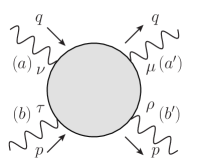
Figure 1: Photon-photon forward scattering with momenta $q(p)$ and helicities $a(b)$ and $a^{\prime}(b^{\prime})$

Let us consider the photon-photon forward scattering amplitude, $\gamma(q,a)+\gamma(p,b)\rightarrow\gamma(q,a^{\prime})+\gamma(p,b^{\prime})$, illustrated in figure 1,

$$T^{\mu\nu\rho\tau}(p,q)=i\int d^{4}xd^{4}yd^{4}ze^{iq\cdot x}e^{ip\cdot(y-z)}\langle 0\left|T({\cal J}^{\mu}(x){\cal J}^{\nu}(0){\cal J}^{\rho}(y){\cal J}^{\tau}(z))\right|0\rangle,$$ (1)

where $q$ and $p$ are four momenta of the probe and target photon, respectively, and ${\cal J}^{\mu}$ is the electromagnetic current. Its absorptive part is related to the structure tensor $W^{\mu\nu\rho\tau}$ as  [16]

$$W^{\mu\nu\rho\tau}=\frac{1}{2\pi}{\rm Im}~{}T^{\mu\nu\rho\tau}.$$ (2)

The s-channel helicity amplitudes are given by

$$W(a^{\prime}b^{\prime}|ab)=\epsilon^{*}_{\mu}(a^{\prime})\epsilon^{*}_{\rho}(b^{\prime})W^{\mu\nu\rho\tau}\epsilon_{\nu}(a)\epsilon_{\tau}(b),$$ (3)

where $\epsilon_{\mu}(a)$ represents the photon polarization vector, and $a,a^{\prime}=0,\pm 1$, and $b,b^{\prime}=\pm 1$. Note that the target photon is real and has no longitudinal mode. Due to the angular momentum conservation, parity conservation, and time reversal invariance, we have in total four independent s-channel helicity amplitudes[17], which we may take as

$$W(1,1|1,1),\quad W(0,1|0,1),\quad W(1,-1|1,-1),\quad W(1,1|-1,-1).$$ (4)

The first three amplitudes are helicity-nonflip and the last one is helicity-flip.

For the real photon target, they appear four photon structure functions, $W_{TT}$, $W_{LT}$, $W_{TT}^{a}$ and $W_{TT}^{\tau}$, which are functions of $Q^{2}(=-q^{2})$ and $x=Q^{2}/(2p\cdot q)$. They also depend on the active quark masses. The subscripts $T$ and $L$ correspond to the transverse and longitudinal photon, respectively. The superscript $``a"$ of $W_{TT}^{a}$ refers to $\mu\nu$ antisymmentric part of $W^{\mu\nu\rho\tau}$, while the superscript $``\tau"$ of $W_{TT}^{\tau}$ refers to transition with spin-flip for each of the photons. These structure functions are related to the s-channel helicity amplitudes as follows;

$$W_{TT} = \frac{1}{2}[W(1,1|1,1)+W(1,-1|1,-1)],$$ (5a)

$$W_{LT} = W(0,1|0,1),$$ (5b)

$$W_{TT}^{a} = \frac{1}{2}[W(1,1|1,1)-W(1,-1|1,-1)],$$ (5c)

$$W_{TT}^{\tau} = W(1,1|-1,-1),$$ (5d)

where $W_{TT}$, $W_{LT}$ and $W_{TT}^{\tau}$ are called as the unpolarized structure functions since they are measured, for example, through the two-photon processes in unpolarized $e^{+}e^{-}$ collision experiments. When polarized $e^{+}$ and $e^{-}$ beams are used, we can get information on the polarized structure function $W_{TT}^{a}$. Other definitions of the photon structure functions are often used, which are $F_{2}^{\gamma}$, $F_{L}^{\gamma}$, $g_{1}^{\gamma}$ and $W_{3}^{\gamma}$ and are related to $W_{i}$’s as follows;

$$\begin{split}F_{2}^{\gamma}=&2x\left[W_{TT}+W_{LT}\right],\quad F_{L}^{\gamma}=2xW_{LT},\\ g_{1}^{\gamma}=&2W_{TT}^{a},\quad W_{3}^{\gamma}=\frac{1}{2}W_{TT}^{\tau}.\end{split}$$ (6)

There exist positivity constraints on the structure functions, which are derived from the Caushy-Schwarz inequality [15] . For the case of real photon, we obtain one positivity constraint as follows;

$$\left|W_{TT}^{\tau}\right|\leq\left|W_{TT}+W_{TT}^{a}\right|.$$ (7)

We will confirm positivity constraint at NLO.

3 Calculation

We calculate the cross sections for the two photon annihilation to the heavy quark $q_{H}{\overline{q}}_{H}$ pairs

$$\gamma^{*}(q)+\gamma(p)\longrightarrow q_{H}+{\overline{q}}_{H}~{},$$ (8)

with one-loop gluon corrections and to the gluon bremsstrahlung processes

$$\gamma^{*}(q)+\gamma(p)\longrightarrow q_{H}+{\overline{q}}_{H}+g~{}.$$ (9)

We employ the technique which is based on the Cutkosky rules  [18] and the reduction of Feynman integrals to master integrals. First, following the Cutkosky rules [19], the delta-functions which appear in the phase space integrals are replaced with differences of two propagators

$$2\pi i\delta(r^{2}-m^{2})\rightarrow\frac{1}{r^{2}-m^{2}+i0}-\frac{1}{r^{2}-m^{2}-i0}~{},$$ (10)

where $m$ is the quark mass. Then the cross sections for the virtual corrections to the processes (8) and for the bremsstrahlung processes (9) are described by the two-loop diagrams shown in figure 3 and figure 3, respectively, where a cut propagator should be understood as the r.h.s. of Eq.(10).

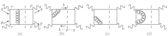
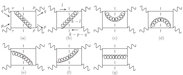
Figure 2: Two-loop diagrams with virtual corrections. Graphs with virtual corrections to the right of the cut lines and graphs with $(q,\mu)$ and $(p,\rho)$ interchanged are added. Graphs with the external quark self-energies are not shown in the figure, but should be included in the calculation.

Figure 3: Two-loop diagrams with a real gluon emission. Similar graphs corresponding to (e) and (f) are included. Also graphs with $(q,\mu)$ and $(p,\rho)$ interchanged are added.

We regularize the amplitudes in dimensional regularization $D=4-2\epsilon$. The absorptive part of the relevant photon-photon scattering amplitude, $W^{\mu\nu\rho\tau}$, can be written as [16]

$$W^{\mu\nu\rho\tau} = (T_{TT})^{\mu\nu\rho\tau}W_{TT}+(T_{LT})^{\mu\nu\rho\tau}W_{LT}+(T_{TT}^{a})^{\mu\nu\rho\tau}W_{TT}^{a}+(T_{TT}^{\tau})^{\mu\nu\rho\tau}W_{TT}^{\tau},$$

where

$$(T_{TT})^{\mu\nu\rho\tau} = R^{\mu\nu}R^{\rho\tau},$$ (12a)

$$(T_{LT})^{\mu\nu\rho\tau} = k_{1}^{\mu}k_{1}^{\nu}R^{\rho\tau},$$ (12b)

$$(T^{a}_{TT})^{\mu\nu\rho\tau} = R^{\mu\rho}R^{\nu\tau}-R^{\mu\tau}R^{\nu\rho},$$ (12c)

$$(T^{\tau}_{TT})^{\mu\nu\rho\tau} = \frac{1}{2}\left(R^{\mu\rho}R^{\nu\tau}+R^{\mu\tau}R^{\nu\rho}-R^{\mu\nu}R^{\rho\tau}\right),$$ (12d)

with

$$R^{\mu\rho}=-g^{\mu\rho}+\frac{q^{\mu}p^{\rho}+q^{\rho}p^{\mu}}{p\cdot q}-\frac{q^{2}p^{\mu}p^{\rho}}{(p\cdot q)^{2}},\quad k_{1}^{\mu}=\sqrt{\frac{-q^{2}}{(p\cdot q)^{2}}}\left(p^{\mu}-\frac{p\cdot q}{q^{2}}q^{\mu}\right)~{}.$$ (13)

We introduce the following $D$-dimensional projection operators

$$(P_{TT})^{\mu\nu\rho\tau}=\frac{3D-8}{2D(D-2)(D-3)}(T_{TT})^{\mu\nu\rho\tau}+\frac{D-4}{D(D-2)(D-3)}(T^{\tau}_{TT})^{\mu\nu\rho\tau}~{},$$ (14a)

$$(P_{LT})^{\mu\nu\rho\tau}=\frac{1}{D-2}(T_{LT})^{\mu\nu\rho\tau}~{},$$ (14b)

$$(P_{TT}^{a})^{\mu\nu\rho\tau}=\frac{1}{2(D-2)(D-3)}(T^{a}_{TT})^{\mu\nu\rho\tau}~{},$$ (14c)

$$(P_{TT}^{\tau})^{\mu\nu\rho\tau}=\frac{D-4}{D(D-2)(D-3)}(T_{TT})^{\mu\nu\rho\tau}+\frac{2}{D(D-3)}(T^{\tau}_{TT})^{\mu\nu\rho\tau}~{},$$ (14d)

such that each structure functions, $W_{TT}$, $W_{LT}$, $W_{TT}^{a}$ and $W_{TT}^{\tau}$, can be extracted by means of the property $(P_{i})^{\mu\nu\rho\tau}(T_{j})_{\mu\nu\rho\tau}=\delta_{ij}$.

We apply the above projection operators to the two-loop diagrams given in figures 3 and 3. The contributions to each structure function are expressed in a linear combination of two-loop scalar integrals of the form

$$A(\nu_{i})\equiv A(\nu_{k},\nu_{kq},\nu_{kp},\nu_{kpq},\nu_{l},\nu_{lq},\nu_{lp},\nu_{lpq},\nu_{kl})$$

$$=\int\frac{d^{D}k}{(2\pi)^{D}}\frac{d^{D}l}{(2\pi)^{D}}\frac{1}{D_{k}^{\nu_{k}}D_{k-q}^{\nu_{kq}}D_{k-p}^{\nu_{kp}}D_{k-p-q}^{\nu_{kpq}}D_{l}^{\nu_{l}}D_{l-q}^{\nu_{lq}}D_{l-p}^{\nu_{lp}}D_{l-p-q}^{\nu_{lpq}}D_{k-l,0}^{\nu_{kl}}}~{},$$

(15)

where

$$D_{p}=p^{2}-m^{2},\qquad D_{p,0}=p^{2}.$$ (16)

Note that $1/D_{k-l,0}$ corresponds to a gluon propagator. The coefficients of these scalar integrals are written as functions of $x,Q^{2},m^{2}$ and $D$. Actually $A(\nu_{i})$ has seven propagators at most and at least two $\nu_{i}$’s are zero. We choose the loop integration variables $k$ and $l$, such that momentum assignment of the cut propagators correspond to $1/D_{k}$ and $1/D_{k-p-q}$ for the diagrams in figure 3 and $1/D_{l}$, $1/D_{k-p-q}$ and $1/D_{k-l,0}$ for the diagrams in figure 3. If $\nu_{i}$’s of the cut propagators are 0 or negative integer, those integrals do not contribute to structure functions due to the Cutkosky rule. Thus we only pick up $A(\nu_{i})$’s which are in the form $A(1,\nu_{kq},\nu_{kp},1,\nu_{l},\nu_{lq},\nu_{lp},\nu_{lpq},\nu_{kl})$ in figure 3 and $A(\nu_{k},\nu_{kq},\nu_{kp},1,1,\nu_{lq},\nu_{lp},\nu_{lpq},1)$ in figure 3. The other scalar integrals are discarded.

There are still a large number of scalar integrals. Next, we apply the reduction procedure [20] and rewrite the scalar integrals in terms of fewer number of master integrals. This procedure is based on the method of integration by parts [21] and the use of the Lorentz invariance of scalar integrals [22]. We make use of FIRE [23], a public reduction code powered by Mathematica, and express the relevant $A(\nu_{i})$s as a linear combination of the master integrals, which are denoted as

$$M(\nu_{i})\equiv M(\nu_{k},\nu_{kq},\nu_{kp},\nu_{kpq},\nu_{l},\nu_{lq},\nu_{lp},\nu_{lpq},\nu_{kl})~{},$$ (17)

in the same way as the notation of $A(\nu_{i})$s in Eq.(15). Again the master integrals in the form of $M(1,\nu_{kq},\nu_{kp},1,\nu_{l},\nu_{lq},\nu_{lp},\nu_{lpq},\nu_{kl})$ are only relevant for the virtual-correction diagrams in figure. 3 and those in the form of $M(\nu_{k},\nu_{kq},\nu_{kp},1,1,\nu_{lq},\nu_{lp},\nu_{lpq},1)$ are relevant for the real-gluon-emission diagrams in figure. 3.

Finally, we perform the phase space integrations by taking discontinuities of the master integrals with cut propagators . For the two-cut and three-cut master integrals, we evaluate

$${\rm Disc}^{(2)}~{}M(1,\nu_{kq},\nu_{kp},1,\nu_{l},\nu_{lq},\nu_{lp},\nu_{lpq},\nu_{kl})$$

$$\equiv\int\frac{d^{D}k}{(2\pi)^{D}}(2\pi)\delta^{(+)}(k^{2}-m^{2})(2\pi)\delta^{(+)}\left((p+q-k)^{2}-m^{2}\right)\frac{1}{D_{k-q}^{\nu_{kq}}D_{k-p}^{\nu_{kp}}}$$

$$\times\int\frac{d^{D}l}{(2\pi)^{D}}\frac{1}{D_{l}^{\nu_{l}}D_{l-q}^{\nu_{lq}}D_{l-p}^{\nu_{lp}}D_{l-p-q}^{\nu_{lpq}}D_{k-l,0}^{\nu_{kl}}}~{},$$

(18)

$${\rm and}$$

$${\rm Disc}^{(3)}~{}M(\nu_{k},\nu_{kq},\nu_{kp},1,1,\nu_{lq},\nu_{lp},\nu_{lpq},1)$$

$$\equiv\int\int\frac{d^{D}k}{(2\pi)^{D}}\int\frac{d^{D}l}{(2\pi)^{D}}~{}(2\pi)\delta^{+}((k-l)^{2})(2\pi)\delta^{+}(l^{2}-m^{2})(2\pi)\delta^{+}((p+q-k)^{2}-m^{2})$$

$$\times\frac{1}{D_{k}^{\nu_{k}}D_{k-q}^{\nu_{kq}}D_{k-p}^{\nu_{kp}}D_{l-q}^{\nu_{lq}}D_{l-p}^{\nu_{lp}}D_{l-p-q}^{\nu_{lpq}}}~{},$$ (19)

respectively, and $M$’s are master integrals which remained after applying reduction algorithm. Note that at least two $\nu_{i}$’s are zero in both (18) and (19). The choice of a set of master integral is not unique and we are at liberty to replace a master integrals with one of other scalar integrals. We choose a set of master integrals such that the coefficients of master integrals are finite in the limit $D\rightarrow 4$ [24]. With this choice of the set, the phase space integrations for master integrals need only be evaluated up to the finite terms in the series expansion in $\epsilon$.

The ultraviolet (UV) singularities appear in the graphs (b), (c) and (d) of figure 3, while the infrared (IR) singularities emerge from the graph (a) of figure 3 and from the real gluon emission graphs (a),(b), (c) and (d) of figure 3. Both the UV and IR singularities are regularized by dimensional regularization. The UV singularities are removed by renormalization. We adopt the on-shell scheme both for the wave function renormalization of the external quark and for the mass renormalization. For the latter, we replace the bare mass in the Born cross section by the renormalized mass $m$,

$$m_{bare}\rightarrow m\left[1+\frac{\alpha_{s}(\mu)}{4\pi}C_{F}S^{\epsilon}\left(\frac{\mu^{2}}{m^{2}}\right)^{\epsilon}\left\{-\frac{3}{\epsilon}-4\right\}\right]~{},$$ (20)

where $\alpha_{s}(\mu)=g^{2}/(4\pi)$ is the QCD running coupling constant, $C_{F}=4/3$ is the Casimir factor and $S^{\epsilon}=(4\pi)^{\epsilon}e^{-\epsilon\gamma_{E}}$ with Euler constant $\gamma_{E}$ and $\mu$ is the arbitrary reference scale of dimensional regularization. The renormalization of the QCD gauge coupling constant is not necessary at this order. The IR singularities cancel when the both contributions from the virtual correction graphs and the real gluon emission graphs are added. Actually the IR singularities reside in the two-cut master integrals in the form $M(1,\nu_{kq},\nu_{kp},1,1,\nu_{lq},\nu_{lp},1,1)$ and the three-cut master integrals $M(\nu_{k},\nu_{kq},\nu_{kp},1,1,\nu_{lq},\nu_{lp},\nu_{lpq},1)$ with $\nu_{k}+\nu_{lpq}=2$.

4 Numerical results

We plot in figures. 4 and 5 the real photon structure functions $W_{TT}(x,Q^{2})$, $W_{LT}(x,Q^{2})$, $W_{TT}^{a}(x,Q^{2})$ and $W_{TT}^{\tau}(x,Q^{2})$ predicted by the massive PM up to the NLO for the case of $Q^{2}=30~{}{\rm GeV}^{2}$. We choose charm and bottom quark as a heavy quark for the figures 4 and 5, respectively. For the running coupling constant, we take $\alpha_{s}=0.21$ choosing $\mu^{2}=Q^{2}$. We take $m_{c}=1.3~{}{\rm GeV}$, $m_{b}=4.5~{}{\rm GeV}$ , $e_{c}=\frac{2}{3}$ and $e_{b}=-\frac{1}{3}$. We show two curves for each structure function: the LO result and the result up to the NLO. The allowed $x$ region is $0\leq x\leq x_{Q}$  with

$$x_{Q}=\frac{1}{1+\frac{4m^{2}}{Q^{2}}}~{}.$$ (21)

The LO results are already known [16] such as

$$W_{TT}^{\rm LO}(x,Q^{2}) = \delta_{q}~{}\Bigl{\{}-\frac{1}{2}\Bigl{(}\ln\frac{1+\beta}{1-\beta}\Bigr{)}\left((\beta^{4}-5)x^{2}-2(\beta^{4}-3)x+\beta^{4}-3\right)$$ (22a)

$$\qquad\quad+\beta\left((\beta^{2}-5)x^{2}-2(\beta^{2}-3)x+\beta^{2}-2\right)\Bigr{\}},$$

$$W^{\rm LO}_{LT}(x,Q^{2}) = \delta_{q}~{}2(1-x)x\Bigl{\{}\Bigl{(}\ln\frac{1+\beta}{1-\beta}\Bigr{)}(\beta^{2}-1)+2\beta\Bigr{\}},$$ (22b)

$$W_{TT}^{a,\rm LO}(x,Q^{2}) = \delta_{q}\Bigl{\{}\Bigl{(}\ln\frac{1+\beta}{1-\beta}\Bigr{)}(2x-1)+\beta(-4x+3)\Bigr{\}},$$ (22c)

$$W_{TT}^{\tau,\rm LO}(x,Q^{2}) = \delta_{q}~{}\Bigl{\{}-\frac{1}{2}\Bigl{(}\ln\frac{1+\beta}{1-\beta}\Bigr{)}(\beta^{2}-1)(x-1)\left((\beta^{2}+3)x-\beta^{2}+1\right)$$ (22d)

$$\qquad\quad+\beta\left((\beta^{2}-3)x^{2}-2(\beta^{2}-1)x+\beta^{2}-1\right)\Bigr{\}},$$

where

$$\beta=\sqrt{1-\frac{4m^{2}x}{Q^{2}(1-x)}}=\sqrt{\frac{1-\frac{x}{x_{Q}}}{1-x}},$$ (23)

and

$$\delta_{q}=\frac{3\alpha}{2\pi}e_{q}^{4}.$$ (24)

For $x\rightarrow x_{Q}$, $\beta$ goes to zero and thus structure functions vanishes at $x_{Q}$ in LO.

We observe that the radiative corrections in NLO are noticeable. In the graphs (a), (c) and (d) of figures. 4 and 5 we find that the radiative corrections to $W_{TT}$, $W_{TT}^{a}$ and $W_{TT}^{\tau}$ are large near the threshold (near $x_{Q}$). Indeed those NLO curves do not vanish at $x_{Q}$. This is due to the Coulomb singularity, which appears when the Coulomb gluon is exchanged between the quark and anti-quark pair near threshold. The diagram figure 3(a) is responsible for this threshold behaviour. The virtual correction to the left of the cut line in figure 3(a) gives rise to a factor $1/\beta$ while a factor $\beta$ comes out from the phase space integration. They are combined and yield a finite but non-zero result at $x_{Q}$. On the other hand, the radiative corrections to $W_{LT}$ shown in the figures  4(b) and 5(b) evade the Coulomb singularity and vanish at threshold. This is because the structure of Coulomb enhancement is given by $W_{i}^{\rm NLO}\sim\left(W_{i}^{\rm LO}\right)\times\alpha_{s}/\beta$ and $W_{LT}^{\rm LO}$ behaves as $\beta^{3}$ for $\beta\rightarrow 0$. Thus $W_{LT}^{\rm NLO}$ vanishes as $\beta^{2}$ near the threshold.

The jump size of Coulomb enhancement for each structure function is calculable in another way. It is well known that the contributions of Coulomb gluons can be summed up to all order. The result of all order resummation is given by Sommerfeld factor. Using Taylor expansion of Sommerfeld factor in strong coupling constant $\alpha_{s}$, leading Coulomb singularity can be reproduced to all order in $\alpha_{s}$. Combining the LO photon structure function $W^{\rm LO}$ with the Sommerfeld factor, we can predict that the jump of the structure function are given by a derivative of LO structure function at the threshold multiplied by $C_{F}\alpha_{s}\pi/2$. That is given by

$$W_{i}^{\rm NLO}(x,Q^{2}) \stackrel{{\scriptstyle\beta\to 0}}{{=}} \left(\beta\left[\frac{dW_{i}^{\rm LO}}{d\beta}\right]_{\beta=0}\right)\times\left(\frac{C_{F}\alpha_{s}\pi}{2\beta}\right)+{\cal O}(\beta),$$ (25)

where part in the first parenthesis corresponds to phase space integration of heavy quark pair and squared LO amplitude and the second is the Coulomb singularity. This formula is assured by the factorization of hard correction and the Coulomb singularities near heavy quark threshold. Our NLO results are consistent with (25) near the threshold. The formula also predict that the NNLO calculation in the massive PM suffers from a divergence, $\beta\times(C_{F}\alpha_{s}/(2\beta))^{2}$, near threshold due to double Coulomb gluon exchange. Therefore fixed order calculation near threshold becomes ill-defined and we need to resort to the method of resummation of the Coulomb singularities. Resummation formulae for the structure functions are given in Appendix A.

For $x\rightarrow 0$, the NLO contributions to $W_{TT}$ and $W_{TT}^{a}$ both diverge. The sum $(W_{TT}+W_{TT}^{a})$ remains finite in LO but diverges in the NLO as $x\rightarrow 0$ [see figure. 6(a) and (b)]. This is due to the collinear divergence. The limiting procedure $x=\frac{Q^{2}}{s+Q^{2}}\rightarrow 0$ with fixed $Q^{2}$ is equivalent of taking $s\rightarrow\infty$. Thus the situation at $x=0$ is the same as if we are dealing with massless quarks. When a gluon is emitted from a massless quark, a collinear divergence appears. We also see in figure. 4(b) the rise of the NLO contributions to $W_{LT}$ near $x=0$, which is again due to the collinear divergence. On the contrary, the LO and NLO contributions to $W_{TT}^{\tau}$ vanishes at $x=0$. A collinear divergence does not occur for the helicity-flip amplitude $W_{TT}^{\tau}$.

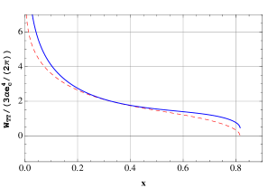
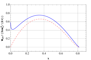
(a) $W_{TT}(x,Q^{2})$	(b) $W_{LT}(x,Q^{2})$
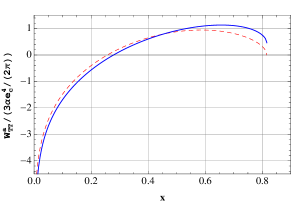
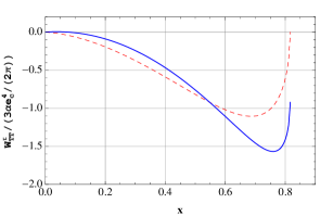
(c) $W_{TT}^{a}(x,Q^{2})$	(d) $W_{TT}^{\tau}(x,Q^{2})$

Figure 4: The charm quark effects on the real photon structure functions (a) $W_{TT}$, (b) $W_{LT}$, (c) $W_{TT}^{a}$ and (d) $W_{TT}^{\tau}$, in the PM for $Q^{2}=30~{}{\rm GeV}^{2}$, $m_{c}=1.3$ GeV and $e_{c}=\frac{2}{3}$ with $\alpha_{s}=0.21$. The vertical axes are in unit of $(3\alpha e_{c}^{4}/(2\pi))$. We plot the LO results (red dotted line) and the results up to the NLO (blue solid line).

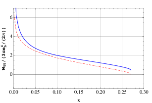
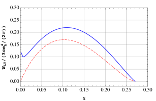
(a) $W_{TT}(x,Q^{2})$	(b) $W_{LT}(x,Q^{2})$
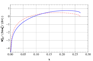
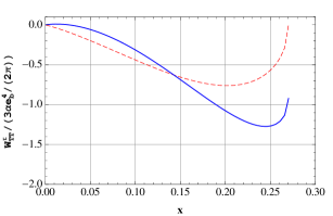
(c) $W_{TT}^{a}(x,Q^{2})$	(d) $W_{TT}^{\tau}(x,Q^{2})$

Figure 5: The bottom quark effects on the real photon structure functions, (a) $W_{TT}$, (b) $W_{LT}$, (c) $W_{TT}^{a}$ and (d) $W_{TT}^{\tau}$, in the PM for $Q^{2}=30~{}{\rm GeV}^{2}$, $m_{b}=4.5$ GeV and $e_{b}=-\frac{1}{3}$ with $\alpha_{s}=0.21$. The vertical axes are in unit of $(3\alpha e_{b}^{4}/(2\pi))$. We plot the LO results (red dotted line) and the results up to the NLO (blue solid line).

We plot the PM predictions of ($W_{TT}+W_{TT}^{a}$) and $|W_{TT}^{\tau}|$ for the case of charm quark in figure 6(a) and for the bottom case in figure 6(b). In both cases we observe that the positivity constraint (7) for a real photon target is satisfied up to the NLO for all the allowed $x$ region with a wide margin except at the threshold $x_{Q}$. At the threshold, we can find the following relation;

$$|W_{TT}^{\tau}(x_{Q},Q^{2})|=W_{TT}(x_{Q},Q^{2})+W_{TT}^{a}(x_{Q},Q^{2}),$$ (26)

At the threshold, we find the following relation (26) from our numerical analysis. This is also checked analytically using resummation formula given in the Appendix A.

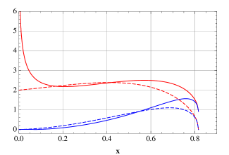
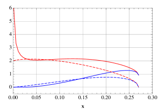
(a) charm quark (b)  bottom quark

Figure 6: The positivity constraint and the PM prediction up to the NLO for $Q^{2}=30~{}{\rm GeV}^{2}$ and $\alpha_{s}=0.21$. (a) Case of charm quark with $m_{c}=1.3$ GeV and $e_{c}=\frac{2}{3}$; (b) Case of bottom quark with $m_{b}=4.5$ GeV and $e_{b}=-\frac{1}{3}$. The vertical axes are in unit of $(3\alpha e_{b}^{4}/(2\pi))$. The result up to the NLO (LO) for ($W_{TT}+W_{TT}^{a}$) is depicted in red solid (red dashed) line. The result up to the NLO (LO) for $|W_{TT}^{\tau}|$ is depicted in blue solid (blue dashed) line.

5 Summary

In this paper, we have investigated heavy quark mass effects for the real photon structure functions in the massive PM in the NLO in QCD. There are four structure functions $W_{TT}$, $W_{LT}$, $W_{TT}^{a}$ and $W_{TT}^{\tau}$ for the real photon target. We have found that the radiative corrections to $W_{TT}$, $W_{TT}^{a}$ and $W_{TT}^{\tau}$ are large near the threshold. This is due to the Coulomb singularity, which appears when the Coulomb gluon is exchanged between the quark and anti-quark pair near threshold. On the other hand, the radiative corrections to $W_{LT}$ evade the Coulomb singularity and vanish at threshold. We also have found that although the sum $(W_{TT}+W_{TT}^{a})$ remains finite in LO but diverges in the NLO as $x\rightarrow 0$. This is due to the collinear divergence. The limiting procedure $x=\frac{Q^{2}}{s+Q^{2}}\rightarrow 0$ with fixed $Q^{2}$ is equivalent of taking the high energy limit $s\rightarrow\infty$. In other words, the situation at $x=0$ corresponds to the massless quark limit. A collinear divergence appears when a gluon is emitted from a massless quark. We also see the collinear divergence in the NLO contributions to $W_{LT}$ near $x=0$. Finally we have shown from the numerical plots of the PM predictions of ($W_{TT}+W_{TT}^{a}$) and $|W_{TT}^{\tau}|$ and the positivity constraint (7) for a real photon target is satisfied for all the allowed $x$ region.

Appendix A Threshold resummation for structure functions

The Green function sums up leading Coulomb singularity for photon-photon forward scattering amplitude. The contribution to the structure function is given by imaginary part of Green function

$${\rm Im}\,G_{C}(\beta)=\frac{m^{2}\beta}{4\pi}\bigg{[}\frac{\frac{C_{F}\alpha_{s}\pi}{\beta}}{1-e^{-\frac{C_{F}\alpha_{s}\pi}{\beta}}}\theta(\beta)+\frac{4\pi}{\beta}\sum_{n=1}^{\infty}a_{n}^{3}\,\delta\left(\beta^{2}+a_{n}^{2}\right)\bigg{]},$$ (27)

with $a_{n}=C_{F}\alpha_{s}/(2n)$. The terms with $\delta$-function are due to Coulomb bound-states, which can have non-zero contribution to the structure functions for $s<4m^{2}$ because $\beta=i\sqrt{4m^{2}/s-1}$ becomes pure imaginary.

We combine the LO photon structure function $W^{\rm LO}$ and the Coulomb Green function $G(\beta)$ [25, 26] in the following form

$$\widehat{W}_{i}^{\rm LO}(x,Q^{2}) = W_{i}^{\rm LO}(x,Q^{2})S(x)+C_{i}\,T(x),$$ (28)

where $S$ encodes the Coulomb singularity and $T$ is the contribution due to boundstate poles. They are defined by

$$S(x) = \frac{C_{F}\alpha_{s}\pi\sqrt{\frac{x_{Q}(1-x)}{x_{Q}-x}}}{1-\exp\left\{-C_{F}\alpha_{s}\pi\sqrt{\frac{x_{Q}(1-x)}{x_{Q}-x}}\right\}}\theta(x_{Q}-x),$$ (29)

$$T(x) = \sum_{n=1}^{\infty}\frac{4\pi a_{n}^{3}x_{Q}(1-x_{Q})}{(1+a_{n}^{2}x_{Q})^{2}}\delta\left(\frac{x_{Q}(1+a_{n}^{2})}{1+a_{n}^{2}x_{Q}}-x\right).$$ (30)

The matching factors are calculable for each structure function as

$$C_{i}=\left\{C_{TT}~{},C_{TT}^{a},~{}C_{TT}^{\tau}\right\}=\left\{1,1,-2\right\}\delta_{q}.$$ (31)

The resummation formula for structure function can be applied for the cases $W_{TT}$, $W_{TT}^{a}$ and $W_{TT}^{\tau}$. Near threshold $W_{LT}$ is order of $\beta^{3}$ at LO, which is suppressed by $\beta^{2}$ compared to $S$-wave case. Therefore its Coulomb singularity at NLO is suppressed by $\beta^{2}$ and the resummation effect becomes moderate.

References

- [1] http://lhc.web.cern.ch/lhc/.
- [2] http://www.linearcollider.org/cms/.
-
[3]
T.F. Walsh, Phys. Lett.36B (1971) 121;
S.J. Brodsky, T. Kinoshita and H. Terazawa, Phys. Rev. Lett.27 (1971) 280. -
[4]
T.F. Walsh and P.M. Zerwas, Phys. Lett.44B (1973) 195;
R.L. Kingsley, Nucl. Phys.60 (1973) 45. - [5] E. Witten, Nucl. Phys. B120, 189 (1977).
-
[6]
W.A. Bardeen and A.J. Buras, Phys. Rev. D20, 166 (1979);
Phys. Rev. D21, 2041 (1980), Erratum;
R.J. DeWitt, L.M. Jones, J.D. Sullivan, D.E. Willen and H.W. Wyld, Jr., Phys. Rev. D19, 2046 (1979); Phys. Rev. D20, 1751 (1979), Erratum;
M. Glück and E. Reya, Phys. Rev. D28, 2749 (1983). -
[7]
S. Moch, J.A.M. Vermaseren and A. Vogt, Nucl. Phys. B621, 413 (2002);
A. Vogt, S. Moch and J.A.M. Vermaseren, Acta Phys. Polon B37, 683 (2006); hep-ph/0511112. - [8] K. Sasaki, Phys. Rev. D22, 2143 (1980); Prog. Theor. Phys. Suppl. 77, 197 (1983).
- [9] M. Stratmann and W. Vogelsang, Phys. Lett. B386, 370 (1996).
-
[10]
M. Glück, E. Reya and C. Sieg, Phys. Lett.
B503, 285 (2001);
Eur. Phys. J. C20, 271 (2001). -
[11]
M. Krawczyk,
AIP Conf. Proc. No.571 (AIP, New York, 2001) and
references therein;
M. Krawczyk, A. Zembrzuski and M. Staszel, Phys. Rept. 345, 265 (2001);
R. Nisius, Phys. Rept. 332, 165 (2001); hep-ex/0110078;
M. Klasen, Rev. Mod. Phys. 74, 1221 (2002);
I. Schienbein, Ann. Phys. 301, 128 (2002);
R. M. Godbole, Nucl. Phys. B (Proc. Suppl.) 126, 414 (2004). - [12] T. Ueda, K. Sasaki and T. Uematsu, Phys. Rev. D75, 114009 (2007).
- [13] E. Laenen, S. Riemersma, J. Smith and W.L. van Neerven, Phys. Rev. D49 (1994) 5753; W. Beenakker, H. Kuijf, W.L. van Neerven and J. Smith, Phys. Rev. D40 (1989) 54.
- [14] N. Watanabe, Y. Kiyo and K. Sasaki, Phys. Lett. B707, 146 (2012).
- [15] K. Sasaki, J. Soffer and T. Uematsu, Phys. Lett. B522, 22 (2001); Phys. Rev. D66, 034014 (2002).
- [16] V.M. Budnev, V.L. Chernyak and I.F. Ginzburg, Nucl. Phys. B34, 470 (1971).
- [17] C. Bourrely, E. Leader, and J. Soffer Phys. Rep 59 (1980) 95.
- [18] C. Anastasiou and K. Melnikov, Nucl. Phys. B646 (2002) 220.
- [19] R.E. Cutkosky, J. Math. Phys. 1 (1960) 429.
- [20] S. Laporta, Int. J. Mod. Phys. A15 (2000) 5087.
- [21] F.V. Tkachov, Phys. Lett. B100 (1981) 65; K.G. Chetyrkin and F.V. Tkachov, Nucl. Phys. B192 (1981) 159.
- [22] T. Gehrmann and E. Remiddi, Nucl. Phys. B580 (2000) 485.
- [23] A.V. Smirnov, JHEP 0810:(2008)107
- [24] K.G. Chetyrkin, M. Faisst, C. Sturm and M. Tentyukov, Nucl. Phys. B742 (2006) 208.
- [25] K. Hagiwara, Y. Sumino and H. Yokoya, Phys. Lett. B666 (2008) 71.
- [26] Y. Kiyo, J.H. Kühn, S. Moch, M. Steinhauser and P. Uwer, Eur. Phys. J. C60 (2009) 375.