Cross-Linked Structure of Network Evolution

Abstract

We study the temporal co-variation of network co-evolution via the cross-link structure of networks, for which we take advantage of the formalism of hypergraphs to map cross-link structures back to network nodes. We investigate two sets of temporal network data in detail. In a network of coupled nonlinear oscillators, hyperedges that consist of network edges with temporally co-varying weights uncover the driving co-evolution patterns of edge weight dynamics both within and between oscillator communities. In the human brain, networks that represent temporal changes in brain activity during learning exhibit early co-evolution that then settles down with practice, and subsequent decreases in hyperedge size are consistent with emergence of an autonomous subgraph whose dynamics no longer depends on other parts of the network. Our results on real and synthetic networks give a poignant demonstration of the ability of cross-link structure to uncover unexpected co-evolution attributes in both real and synthetic dynamical systems. This, in turn, illustrates the utility of analyzing cross-links for investigating the structure of temporal networks.

Networks provide a useful framework for gaining insights into a wide variety of social, physical, technological, and biological phenomena Newman (2010). As time-resolved data become more widely available, it is increasingly important to investigate not only static networks but also temporal networks Holme and Saramäki (2012, 2013). It is thus critical to develop methods to quantify and characterize dynamic properties of nodes (which represent entities) and/or edges (which represent ties between entities) that vary in time. In the present paper, we describe methods for the identification of cross-link structures in temporal networks by isolating sets of edges with similar temporal dynamics. We use the formalism of hypergraphs to map these edge sets to network nodes, thereby describing the complexity of interaction dynamics in system components. We illustrate our methodology using temporal networks that we extracted from synthetic data generated from coupled nonlinear oscillators and empirical data from human brain activity.

I Introduction

Many complex systems can be represented as temporal networks, which consist of components (i.e., nodes) that are connected by time-dependent edges Holme and Saramäki (2012, 2013). The edges can appear, disappear, and change in strength over time. To obtain a deep understanding of real and model networked systems, it is critical to try to determine the underlying drivers of such edge dynamics. The formalism of temporal networks provides a means to study dynamic phenomena in biological Bassett et al. (2011, 2013a); Wymbs et al. (2012), financial Fenn et al. (2009, 2011), political Waugh et al. (2012); Mucha et al. (2010); Macon et al. (2012), social Fararo and Skvoretz (1997); Stomakhin et al. (2011); Onnela et al. (2007); Wu et al. (2010); González-Bailón et al. (2011); Christakis and Fowler (2007); Snijders et al. (2007) systems, and more.

Capturing salient properties of temporal edge dynamics is critical for characterizing, imitating, predicting, and manipulating system function. Let’s consider a system that consists of the same $N$ components for all time. One can parsimoniously represent such a temporal network as a collection of edge-weight time series. For undirected networks, we thus have a total of $N(N-1)/2$ time series, which are of length $T$. The time series can either be inherently discrete or they can be obtained from a discretization of continuous dynamics (e.g., from the output of a continuous dynamical system). In some cases, the edge weights that represent the connections are binary, but this is not true in general.

Several types of qualitative behavior can occur in time series that represent edge dynamics Slotine and Liu (2012); Nepusz and Vicsek (2012). For example, unvarying edge weights are indicative of a static system, and independently varying edge weights indicate that a system does not exhibit meaningfully correlated temporal dynamics. A much more interesting case, however, occurs when there are meaningful transient or long-memory dynamics. As we illustrate in this article, one can obtain interesting insights in such situations by examining network cross-links, which are defined via the temporal co-variation in edge weights. Illuminating the structure of cross-links has the potential to enable predictability.

To gain intuition about the importance of analyzing cross-links, it is useful to draw an analogy from biology. The cellular cytoskeleton Peters (1963) is composed of actin filaments that form bridges (edges) between different parts (nodes) of a cell. Importantly, the bridges are themselves linked to one another via actin-binding proteins. Because the network edges in this system are not independent of each other, the structure of cross-links has important implications for the mechanical and transport properties of the cytoskeleton. Similarly, one can think of time-dependent relationships between edge weights as cross-links that might change the temporal landscape for dynamic phenomena like information processing, social adhesion, and systemic risk. Analyzing cross-links allows one to directly investigate time-dependent correlations in a system, and it thereby has the potential to yield important insights on the (time-dependent) structural integrity of a diverse variety of systems.

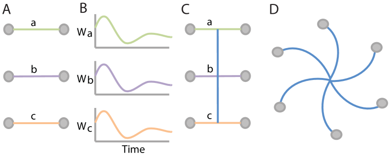
Figure 1: Co-Evolution Cross-Links and Hyperedges. A set of (A) node-node edges with (B) similar edge-weight time series are (C) cross-linked to one another, which yields (D) a hyperedge that connects them.

In this article, we develop a formalism for uncovering the structure in time-dependent networks by extracting groups of edges that share similar temporal dynamics. We map these cross-linked groups of edges back to the nodes of the original network using hypergraphs Bollobás (1998). We define a co-evolution hypergraph via a set of hyperedges that captures cross-links between network edges, where each hyperedge is given by the set of edges that exhibit statistically significant similarities to one another in the edge-weight time series (see Fig. 1). A single temporal network can contain multiple hyperedges, and each of these can capture a different temporal pattern of edge-weight variation.

We illustrate our approach using ensembles of time-dependent networks extracted from a nonlinear oscillator model and empirical neuroscience data.

II Cross-Link Structure

To quantify network co-evolution, we extract sets of edges whose weights co-vary in time. For a temporal network $\bf{A}_{t}$, where each $t$ indexes a discrete sequence of $N\times N$ adjacency matrices, we calculate the $E\times E$ adjacency matrix ${\bf\Lambda}$, where the matrix element $\Lambda_{ab}$ is given by the Pearson correlation coefficient between the time series of weights for edge $a$ and that for edge $b$. Note that $E=N(N-1)/2$ is the total number of possible (undirected) edges per layer in a temporal network. The layers can come from several possible sources: data can be inherently discrete, so that each layer represents connections at a single point in time; the output of a continuous system can be discretized (e.g., via constructing time windows); etc. We identify the statistically significant elements of the edge-edge correlation matrix ${\bf\Lambda}$ (see the Supplementary Material ), and we retain these edges (with their original weights) in a new matrix ${\bf\Lambda^{\prime}}$. We set all other elements of ${\bf\Lambda^{\prime}}$ to $0$.

We examine the structure of the edge-edge co-variation represented by the $E\times E$ matrix ${\bf\Lambda^{\prime}}$ by identifying sets of edges that are connected to one another by significant temporal correlations (i.e., by identifying cross-links; see Fig. 1). If ${\bf\Lambda^{\prime}}$ contains multiple connected components, then we study each component as a separate edge set. If ${\bf\Lambda^{\prime}}$ contains a single connected component, then we extract edge sets using community detection. (See the Supplementary Material [24] for a description of the community-detection techniques that we applied to the edge-edge association matrix.) We represent each edge set as a hyperedge, and we thereby construct a co-evolution hypergraph $\bf{H}$. The nodes are the original $N$ nodes in the temporal network, and they are connected via a total of $\eta$ hyperedges that we identified from ${\bf\Lambda^{\prime}}$. The benefit of treating edge communities as hyperedges is that one can then map edge communities back to the original network nodes. This, in turn, makes it possible to capture properties of edge-weight dynamics by calculating network diagnostics on these nodes.

Diagnostics. To evaluate the structure of co-evolution hypergraphs, we compute several diagnostics. To quantify the extent of co-evolution, we define the strength of co-variation as the sum of all elements in the edge-edge correlation matrix: $\nu_{A_{t}}=\sum_{a,b}\Lambda^{\prime}_{ab}$. To quantify the breadth of a single co-variation profile, we define the size of a hyperedge as the number of cross-links that comprise the hyperedge: $s(h)=\frac{1}{2}\sum_{a,b\in\lambda}[\Lambda^{\prime}_{ab}>0]_{\lambda}$, where the square brackets denote a binary indicator function (i.e., 1 if is true and 0 if it is false) and $\lambda$ indicates the set of edges that are present in the hyperedge $h$ of the matrix ${\bf\Lambda^{\prime}}$. To quantify the prevalence of hyperedges in a single node in the network, we define the hypergraph degree of a node $i$ to be equal to the number of hyperedges $\eta_{i}$ associated with node $i$.

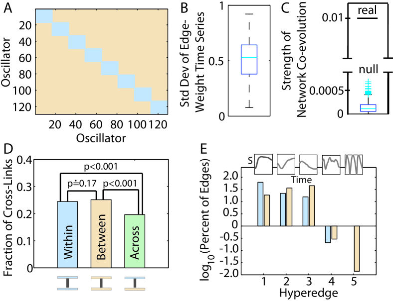
Figure 2: Co-evolution Properties of Kuramoto Oscillator Network Dynamics. (A) Community structure in a network of Kuramoto oscillators. (B) A box plot of the standard deviation in edge weights over time for a temporal network of Kuramoto oscillators. (C) Strength of network co-evolution $\nu_{A_{t}}$ of the real temporal network and a box plot indicating the distribution of $\nu_{A_{t}}$ obtained from 1000 instantiations of a null-model network. (D) Fraction of significant edge-edge correlations (i.e., cross-links) that connect a pair of within-community edges (“Within”), that connect a pair of between-community edges (“Between”), and that connect a within-community edge to a between-community edge (“Across”). We calculated the statistical significance of differences in these fraction values across the 3 cross-link types by permuting labels uniformly at random between each type of pair. (E) Fraction of (blue) within-community and (peach) between-community edges in each of the 5 edge sets extracted from ${\bf\Lambda^{\prime}}$ using community detection. We give values on a logarithmic scale. Insets Mean synchronization [$S(t)=\sum_{(i,j)\in h}A_{ij}(t)$] of these edges as a function of time for each hyperedge $h$.

III Networks of Nonlinear Oscillators

Synchronization provides an example of network co-evolution, as the coherence (represented using edges) between many pairs of system components (nodes) can increase in magnitude over time Pikovsky and Rosenblum (2007); Pikovsky et al. (2003). Pairs of edge-weight time series exhibit temporal co-variation (i.e., they have nontrivial cross-links) because they experience such a trend. Perhaps less intuitively, nontrivial network co-evolution can also occur even without synchronization. To illustrate this phenomenon, we construct temporal networks from the time-series output generated by interacting Kuramoto oscillators Kuramoto (1984), which are well-known dynamical systems that have been studied for their synchronization properties (both with and without a nontrivial underlying network structure) Strogatz (2000); Pikovsky and Rosenblum (2007); Pikovsky et al. (2003); Arenas et al. (2008); Shima and Kuramoto (2004); Abrams and Strogatz (2004); Arenas et al. (2006); Stout et al. (2011). By coupling Kuramoto oscillators on a network with community structure Arenas et al. (2006), we can probe the co-evolution of edge weight time series both within and between synchronizing communities.

In Fig. 2A, we depict the block-matrix community structure in a network of $128$ Kuramoto oscillators with $8$ equally-sized communities. The phase $\theta_{i}(t)$ of the $i^{\mathrm{th}}$ oscillator evolves in time according to

$$\frac{d\theta_{i}}{dt}=\omega_{i}+\sum_{j}\kappa C_{ij}\mathrm{sin}(\theta_{j}-\theta_{i})\,,\quad i\in\{1,\ldots,N\}\,,$$ (1)

where $\omega_{i}$ is the natural frequency of oscillator $i$, the matrix $\mathbf{C}$ gives the binary-valued ($0$ or $1$) coupling between each pair of oscillators, and $\kappa$ (which we set to $0.2$) is a positive real constant that indicates the strength of the coupling. We draw the frequencies $\omega_{i}$ from a Gaussian distribution with mean $0$ and standard deviation $1$. Each node is connected to 13 other nodes (chosen uniformly at random) in its own community and to one node outside of its community. This external node is chosen uniformly at random from the set of all nodes from other communities.

To quantify the temporal evolution of synchronization patterns, we define a set of temporal networks from the time-dependent correlations (which, following Ref. Arenas et al. (2006), we use to measure synchrony) between pairs of oscillators: $A_{ij}(t)=\left\langle|\cos[\theta_{i}(t)-\theta_{j}(t)]|\right\rangle$, where the angular brackets indicate an average over $20$ simulations. We perform simulations, each of which use a different realization of the coupling matrix $\mathbf{C}$ (see the Supplementary Material [24] for details of the numerics). Importantly, edge weights not only vary (see Fig. 2B) but they also co-vary with one another (see Fig. 2C) in time: the strength of network co-evolution, which we denote by $\nu_{A_{t}}$, is greater than that expected in a null-model network in which each edge-weight time series is independently permuted uniformly at random.

In this example, the cross-links given by the non-zero elements of ${\bf\Lambda^{\prime}}$ form a single connected component due to the extensive co-variation. One can distinguish cross-links according to their roles relative to the community structure in Fig. 2A Guimerà and Amaral (2005): (i) pairs of within-community edges, (ii) pairs of between-community edges, and (iii) pairs composed of one within-community edge and one between-community edge. Assortative pairings [i.e., cases (i) and (ii)] are significantly more represented than disassortative pairings [i.e., case (iii)] (see Fig. 2D). The assortative nature of cross-links might be driven by the underlying community structure in the block structure in Fig. 2A: within-community edges are directly connected to one another via shared nodes, whereas between-community edges are more distantly connected to one another via a common input (e.g., a sparse but frequently updating representation of the state of other oscillators).

Using community detection, we identified 5 distinct edge sets (i.e., hyperedges) in ${\bf\Lambda^{\prime}}$ with distinct temporal profiles (see Fig. 2E). The first hyperedge tends to connect within-community edges to each other. On average, they tend to synchronize early in our simulations. The second and third hyperedges tend to connect between-community edges to each other. The second hyperedge connects edges that tend to exhibit a late synchronization, and the third one connects edges that tend to exhibit an initial synchronization followed by a desynchronization. The fourth and fifth hyperedges are smaller in size (i.e., contain fewer edges) than the first three, and their constituent edges oscillate between regimes with high and low synchrony. The edges that constitute the fifth hyperedge oscillate at approximately one frequency, whereas those in the fourth hyperedge have multiple frequency components. See the Supplementary Material [24] for a characterization of the temporal profiles and final synchronization patterns of hyperedges in the network of Kuramoto oscillators.

Together, our results demonstrate the presence of multiple co-evolution profiles: early synchronization, late synchronization, desynchronization, and oscillatory behavior Arenas et al. (2008). Moreover, the assortative pairing of cross-links indicates that temporal information in this dynamic system is segregated not just within separate synchronizing communities but also in between-community edges.

IV Networks of Human Brain Areas

Our empirical data captures the changes in regional brain activity over time as experimental subjects learn a complex motor-sequencing task that is analogous to playing complex keyboard arpeggios. Twenty individuals practiced on a daily basis for 6 weeks, and we acquired MRI brain scans of blood oxygenated-level-dependent (BOLD) signal at four times during this period. We extracted time series of MRI signals from $N=112$ parts of each individual’s brain Bassett et al. (2013b). Co-variation in BOLD measurements between brain areas can indicate shared information processing, communication, or input; and changes in levels of coherence over time can reflect the network structure of skill learning. We summarize such functional connectivity Friston (1994) patterns using an $N\times N$ coherence matrix Bassett et al. (2011, 2013a), which we calculate for each experimental block. We extract temporal networks, which each consist of 30 time points, for naive (experimental blocks corresponding to 0–50 trials practiced), early (60–230), middle (150–500), and late (690–2120) learning Bassett et al. (2013b). We hypothesize that learning should be reflected in changes of hypergraph properties over the very long time scales (6 weeks) associated with this experiment.

Temporal brain networks exhibit interesting dynamics: all four temporal networks exhibit a non-zero variation in edge weights over time (see Fig. 3A). Importantly, edge weights not only vary but co-vary in time: the strength of network co-evolution $\nu_{A_{t}}$ is greater in the 4 real temporal networks than expected in a random null-model network in which each edge-weight time series is independently permuted uniformly at random (see Fig. 3B). The magnitude of temporal co-variation between functional connections is modulated by learning: it is smallest prior to learning and largest during early learning (i.e., amidst most performance gains). These results are consistent with the hypothesis that the adjustment of synaptic weights during learning alters the synchronization properties of neurophysiological signals Bassett et al. (2011), which could manifest as a steep gain in the co-evolution of synchronized activity of large-scale brain areas.

To uncover groups of co-evolving edges, we study the edge-edge correlation matrix ${\bf\Lambda^{\prime}}$, whose density across the 4 temporal networks and the 20 study participants ranged from approximately 1% to approximately 95%. We found that the significant edges were already associated with multiple connected components, so we did not further partition the edge sets into communities. The distribution of component sizes $s$ is heavy-tailed (see Fig. 3C), which perhaps reflects inherent variation in the communication patterns that are necessary to perform multiple functions required during learning Bassett et al. (2011). With long-term training, hyperedges decrease in size (see Fig. 3C), which might reflect an emerging autonomy of sensorimotor regions that can support sequential motor behavior without relying on association cortex.

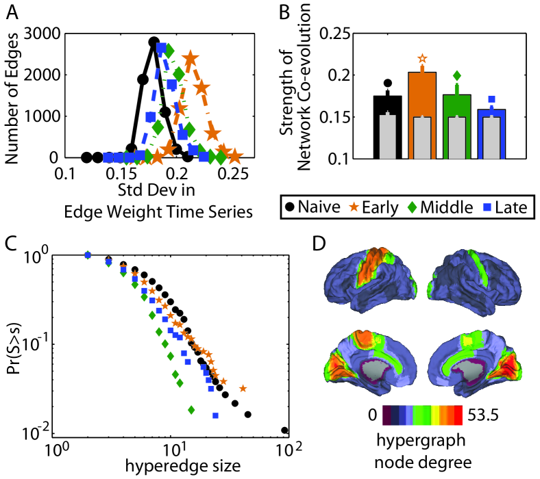
Figure 3: Co-evolution Properties of Brain Network Dynamics. (A) A histogram of the number of edges as a function of the standard deviation in edge weights over time for the 4 temporal networks. (B) Strength of network co-evolution $\nu_{A_{t}}$ of 4 temporal networks and the respective null-model networks (gray). Error bars indicate standard deviation of the mean over study participants. (C) Cumulative probability distribution $Pr$ of the size $s$ of hyperedges in the 4 learning hypergraphs. (D) Anatomical distribution of early-learning hypergraph node degree (averaged over the 20 participants). We obtain qualitatively similar results from the early, middle, late, and extended learning temporal networks. In panels (A-C), color and shape indicate the temporal network corresponding to (black circles) naive, (orange stars) early, (green diamonds) middle, and (blue squares) late learning.

Hyperedges indicate temporal co-variation of putative communication routes in the brain and can be distributed across different anatomical locations. The hypergraph node degree quantifies the number of hyperedges that are connected to each brain region. We observe that nodes with high hypergraph degree are located predominantly in brain regions known to be recruited in motor sequence learning Dayan and Cohen (2011): the primary sensorimotor strip in superior cortex and the early visual areas located in occipital cortex (see Fig. 3D).

V Methodological Considerations & Future Directions

The approach that we have proposed in this paper raises several interesting methodological questions that are worth additional study.

First, there are several ways (e.g., using the edge-edge correlation matrix ${\bf\Lambda}$) to define the statistical significance of a single element in a large matrix that is constructed from correlations or other types of statistical similarities between time series (see the Supplementary Material [24]). Naturally, one should not expect that there is a single “best-choice” correction for false-positive (i.e., Type I) errors in these matrices that is applicable to all systems, scales, and types of association. In the future, rather than using a single threshold for statistical significance to convert ${\bf\Lambda}$ to ${\bf\Lambda^{\prime}}$, it might be advantageous to use a range of thresholds — perhaps to differentially probe strong and weak elements of a correlation matrix, as has been done in the neuroimaging literature Bassett et al. (2012) — to characterize the organization of the hypergraphs on different geometrical scales (i.e., for different distributions of edge-weight values).

Second, the dependence of the hypergraph structure on the amount of time $T$ that we consider is also a very interesting and worthwhile question. Intuitively, the hypergraph structure seems to capture transient dependencies between edges for small $T$ but to capture persistent dependencies between edges for large $T$. A detailed probing of the $T$-dependence of the hypergraph structure could be particularly useful for studying systems that exhibit (i) temporally-independent state transitions based on their cross-linked structures and (ii) co-evolution dynamics that occur over multiple temporal scales.

Finally, the approach that we have proposed in this paper uses hypergraphs to connect dependencies between interactions to the components that interact. Alternatively, one can construe the interactions themselves as one network and the components that interact as a second network. This yields a so-called interconnected network (which is a type of multilayer network Kivelä et al. (2013)), and the development of techniques to study such networks is a burgeoning area of research. Using this lens makes it clear that our approach can also be applied “in the other direction” to connect sets of components that exhibit similar dynamics (one network) to interactions between those components (another network). This yields a simple multilayer structure in which a single set of components is connected by two sets of associations (similarities in dynamics and via a second type of interaction). However, we believe that the “forward” direction that we have pursued is the more difficult of the two directions, as one needs to connect a pair of networks whose edges are defined differently and whose nodes are also defined differently. Hypergraphs provide one solution to this difficulty because they make it possible to bridge these two networks. Moreover, many dynamical systems include both types of networks: a network that codifies dependencies between nodes and a network that codifies dependencies between node-node interactions.

Conclusion

Networked systems are ubiquitous in technology, biology, physics, and culture. The development of conceptual frameworks and mathematical tools to uncover meaningful structure in network dynamics is critical for the determination and control of system function. We have demonstrated that the cross-link structure of network co-evolution, which can be represented parsimoniously using hypergraphs, can be used to identify unexpected temporal attributes in both real and simulated temporal dynamical systems. This, in turn, illustrates the utility of analyzing cross-links for investigating the structure of temporal networks.

References

- Newman (2010) M. E. J. Newman, Networks: An Introduction (Oxford University Press, 2010).
- Holme and Saramäki (2012) P. Holme and J. Saramäki, Phys Rep 519, 97 (2012).
- Holme and Saramäki (2013) P. Holme and J. Saramäki, eds., Temporal Networks (Springer, 2013).
- Bassett et al. (2011) D. S. Bassett, N. F. Wymbs, M. A. Porter, P. J. Mucha, J. M. Carlson, and S. T. Grafton, Proc Natl Acad Sci USA 108, 7641 (2011).
- Bassett et al. (2013a) D. S. Bassett, M. A. Porter, N. F. Wymbs, S. T. Grafton, J. M. Carlson, and P. J. Mucha, Chaos 23, 013142 (2013a).
- Wymbs et al. (2012) N. F. Wymbs, D. S. Bassett, P. J. Mucha, M. A. Porter, and S. T. Grafton, Neuron 74, 936 (2012).
- Fenn et al. (2009) D. J. Fenn, M. A. Porter, M. McDonald, S. Williams, N. F. Johnson, and N. S. Jones, Chaos 19, 033119 (2009).
- Fenn et al. (2011) D. J. Fenn, M. A. Porter, S. Williams, M. McDonald, N. F. Johnson, and N. S. Jones, Phys Rev E 84, 026109 (2011).
- Waugh et al. (2012) A. S. Waugh, L. Pei, J. H. Fowler, P. J. Mucha, and M. A. Porter, “Party polarization in Congress: A network science approach,” (2012), arXiv:0907.3509.
- Mucha et al. (2010) P. J. Mucha, T. Richardson, K. Macon, M. A. Porter, and J.-P. Onnela, Science 328, 876 (2010).
- Macon et al. (2012) K. T. Macon, P. J. Mucha, and M. A. Porter, Physica A 391, 343 (2012).
- Fararo and Skvoretz (1997) T. J. Fararo and J. Skvoretz, in Status, Network, and Structure: Theory Development in Group Processes (Stanford University Press, 1997) pp. 362–386.
- Stomakhin et al. (2011) A. Stomakhin, M. B. Short, and A. L. Bertozzi, Inverse Prob 27, 115013 (2011).
- Onnela et al. (2007) J.-P. Onnela, J. Saramäki, J. Hyvönen, G. Szabó, D. Lazer, K. Kaski, J. Kertész, and A. L. Barabási, Proc Natl Acad Sci USA 104, 7332 (2007).
- Wu et al. (2010) Y. Wu, C. Zhou, J. Xiao, J. Kurths, and H. J. Schellnhuber, Proc Natl Acad Sci USA 107, 18803 (2010).
- González-Bailón et al. (2011) S. González-Bailón, J. Borge-Holthoefer, A. Rivero, and Y. Moreno, Sci Rep 1, 197 (2011).
- Christakis and Fowler (2007) N. A. Christakis and J. H. Fowler, New Eng. J. Med. 357, 370 (2007).
- Snijders et al. (2007) T. A. B. Snijders, C. E. G. Steglich, and M. Schweinberger, in Longitudinal Models in the Behavioral and Related Sciences, edited by K. Van Montfort, H. Oud, and A. Satorra (Lawrence Erlbaum, 2007) pp. 41–71.
- Slotine and Liu (2012) J.-J. Slotine and Y.-Y. Liu, Nat Phys 8, 512 (2012).
- Nepusz and Vicsek (2012) T. Nepusz and T. Vicsek, Nat Phys 8, 568 (2012).
- Peters (1963) R. A. Peters, Biochemical Lesions and Lethal Synthesis (Pergamon Press, Oxford, 1963).
- Bollobás (1998) B. Bollobás, Modern Graph Theory (Springer Verlag, 1998).
- Note (1) In this paper, we use the term co-evolution to indicate temporal co-variation of edge weights in time. The term co-evolution has also been used in other contexts in network science (e.g., Xie et al. (2007); Kim and Goh (2013)).
- Note (2) Supplementary Material for this manuscript can be found at [URL will be inserted by AIP].
- Pikovsky and Rosenblum (2007) A. Pikovsky and M. Rosenblum, Scholarpedia 2, 1459 (2007).
- Pikovsky et al. (2003) A. Pikovsky, M. Rosenblum, and J. Kurths, Synchronization: A Universal Concept in Nonlinear Sciences (Cambridge University Press, 2003).
- Kuramoto (1984) Y. Kuramoto, Chemical Oscillations, Waves, and Turbulence (Springer-Verlag, 1984).
- Strogatz (2000) S. H. Strogatz, Physica D 143, 1 (2000).
- Arenas et al. (2008) A. Arenas, A. Díaz-Guilera, J. Kurths, Y. Moreno, and C. Zhou, Phys Rep 469, 93 (2008).
- Shima and Kuramoto (2004) S. I. Shima and Y. Kuramoto, Phys Rev E 69, 036213 (2004).
- Abrams and Strogatz (2004) D. M. Abrams and S. H. Strogatz, Phys Rev Lett 93, 174102 (2004).
- Arenas et al. (2006) A. Arenas, A. Díaz-Guilera, and C. J. Pérez-Vicente, Phys Rev Lett 96, 114102 (2006).
- Stout et al. (2011) J. Stout, M. Whiteway, E. Ott, M. Girvan, and T. M. Antonsen, Chaos 21, 025109 (2011).
- Guimerà and Amaral (2005) R. Guimerà and L. A. N. Amaral, Nature 433, 895 (2005).
- Bassett et al. (2013b) D. S. Bassett, N. F. Wymbs, M. P. Rombach, M. A. Porter, P. J. Mucha, and S. T. Grafton, PLOS Comp Biol 9, e1003171 (2013b).
- Friston (1994) K. J. Friston, Hum Brain Mapp 2, 56 (1994).
- Dayan and Cohen (2011) E. Dayan and L. G. Cohen, Neuron 72, 443 (2011).
- Bassett et al. (2012) D. S. Bassett, B. G. Nelson, B. A. Mueller, J. Camchong, and K. O. Lim, Neuroimage 59, 2196 (2012).
- Kivelä et al. (2013) M. Kivelä, M. A. Arenas, M. Barthelemy, J. P. Gleeson, Y. Moreno, and M. A. Porter, “Multilayer networks,” (2013), arXiv:1309.7233.
- Xie et al. (2007) Y. B. Xie, W. X. Wang, and B. H. Wang, Phys Rev E 75, 026111 (2007).
- Kim and Goh (2013) J. Y. Kim and K.-I. Goh, Phys. Rev. Lett. 111, 058702 (2013).