The Fermi volume as a probe of hidden order

Abstract

We demonstrate that the volume of the Fermi surface, measured very precisely using de Haas-van Alphen oscillations, can be used to probe changes in the nature and occupancy of localized electronic states. In systems with unconventional ordered states, this allows an underlying electronic order parameter to be followed to very low temperatures. We describe this effect in the field-induced antiferroquadrupolar (AFQ) ordered phase of PrOs₄Sb₁₂, a heavy fermion intermetallic compound. We find that the phase of de Haas-van Alphen oscillations is sensitively coupled, through the Fermi volume, to the configuration of the Pr $f$-electron states that are responsible for AFQ order. In particular, the $\beta$-sheet of the Fermi surface expands or shrinks as the occupancy of two competing localized Pr crystal field states changes. Our results are in good agreement with previous measurements, above 300 mK, of the AFQ order parameter by other methods. In addition, the low temperature sensitivity of our measurement technique reveals a strong and previously unrecognized influence of hyperfine coupling on the order parameter below 300 mK within the AFQ phase. Such hyperfine couplings could provide insight into the nature of hidden order states in other systems.

I Introduction

Studies of correlated electron systems have led to the discovery of many novel ordered phases, sometimes characterized by subtle broken symmetries. It is often challenging, however, to understand these ordered phases, as it is a common problem that no experimental probe couples in a simple way to the microscopic order parameter. This makes it difficult to determine how the order manifests itself in terms of the quantum states of the electrons, and sometimes even to determine how strong the order is. For example, the true nature of spin arrangements in antiferromagnets was “hidden” for several decades, until the development of neutron diffraction as a probe that couples to the order parameter Shull et al. (1951). There are several modern examples of hidden order, which are among the most active topics of investigation in the field of strongly correlated electron systems. These include electronic nematics – states that are characterized macroscopically as translationally invariant electronic states that break the rotational symmetry of a crystal – and exotic superconducting states. It is believed that nematic states arise from fluctuating density waves, but in systems of interest such as the bi-layer ruthenate Sr₃Ru₂O₇, quantum Hall systems, and some cuprate and iron-pnictide superconductors, the microscopic nature of these broken-symmetry electronic states has not been directly observed Fradkin et al. (2010). In systems such as the heavy fermion superconductor UPt₃, the order parameter can be difficult to determine, because there are no available probes that couple directly to the gap function Joynt and Taillefer (2002).

Electric multipole order of the kind observed in PrOs₄Sb₁₂ is a type of hidden order widely observed in $f$-electron materials Hanzawa and Kasuya (1984); Yamauchi et al. (1999); Morin and Schmitt (1990), in which the electron density around some atoms in the unit cell spontaneously distorts in a repeating pattern throughout the crystal. The change in electron density is a very small perturbation of the total electron density, so that traditional probes such as x-rays couple only very weakly. Neutron scattering may couple indirectly to multipolar order if there is an admixture of magnetic dipole as well as charge order, or if there is a sufficiently large lattice distortion Walker et al. (1994) but there are cases of quadrupolar order where neutron diffraction patterns are unchanged upon entry into an AFQ phase Yamauchi et al. (1999). A well-known example of a system with hidden order that may be due to multipolar charge ordering is URu₂Si₂, for which several different varieties of multipolar order, from quadrupolar to hexadecapolar, as well as a number of other scenarios, have been proposed Mydosh and Oppeneer (2011). Here, we show that precise measurements of the volume of the Fermi surface can reflect the modified charge density of multipolar-ordered states, allowing such order to be measured at very low temperatures.

In multipolar order, degenerate or nearly degenerate localized electronic states form superpositions that lower the energy of the ground state. In PrOs₄Sb₁₂, the material we study, antiferroquadrupolar (AFQ) order arises in the doubly occupied $4f$-electron shell of the Pr ions. The AFQ phase appears for applied magnetic fields between about 4 and 12 T and temperatures below $\sim$1 K Aoki et al. (2002a) (the green region in Fig. 1a) and is understood as follows Shiina (2004). In the skutterudite crystal structure of PrOs₄Sb₁₂, shown in Fig. 1c, the $J=4$ spin-orbit-coupled ground state of a Pr 4$f^{2}$ state feels the electric field of the surrounding cage of 12 Sb ions, lifting the 9-fold degeneracy it would have in free space. The resulting localized crystal field states have a ground state singlet, labeled $\Gamma_{1}$, and a very low-lying triplet, labeled $\Gamma_{4}^{(2)}$. (The admixtures of the various $|J,J_{z}\rangle$ states in $\Gamma_{1}$ and $\Gamma_{4}^{(2)}$ are given in references Aoki et al. (2002a); Kohgi et al. (2003); Shiina (2004); Shiina and Aoki (2004).) All other crystal-field levels are at much higher energies and can be ignored. (For more details see Appendix 2.)

Application of a magnetic field causes the ground state to acquire a small admixture of the $m_{z}=0$ triplet state, $\Gamma_{4}^{(2),0}$, and, more importantly, it splits the $m_{z}=\pm 1$ members of the triplet state, so that the spin-up branch of the triplet, $\Gamma_{4}^{(2),+}$, crosses $\Gamma_{1}$ near 8 T Shiina (2004); Aoki et al. (2002a), as shown schematically in Fig. 1b. The charge distributions for $\Gamma_{1}$ and $\Gamma_{4}^{(2),+}$ are pictured in Fig. 1d. A weak nearest-neighbour interaction between the quadrupole moments of these distributions, combined with the near-degeneracy of $\Gamma_{1}$ and $\Gamma_{4}^{(2),+}$ close to 8 T, leads to the new AFQ ground-state in which there is an electric quadrupole moment that alternates on neighbouring sublattices, due to a coherent superposition of the $\Gamma_{1}$ and $\Gamma_{4}^{(2)}$ states on each site. Within mean-field theory, this superposition would have the form $\sum_{i,j}a_{i,j}|\Gamma_{4}^{(2),j}\rangle+b_{i}|\Gamma_{1}\rangle$, where $i=1,2$ is a sublattice index and $j=+,0,-$ sums over the three states in the triplet. Outside the AFQ phase, in contrast, the $\Gamma_{1}$ and $\Gamma_{4}^{(2),+}$ states would be randomly populated according to the Boltzmann distribution as indicated in Fig. 1(a). Both within and outside the AFQ phase, the occupancies of $\Gamma_{1}$ and $\Gamma_{4}^{(2),+}$ change rapidly with field and temperature.

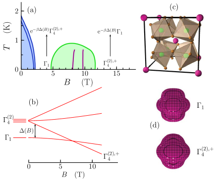
Figure 1: Antiferroquadrupolar order in PrOs₄Sb₁₂. (a) $B-T$ phase diagram of PrOs₄Sb₁₂, based on reference Tayama et al. (2003). The blue region is superconducting, with a double superconducting transition indicated by the blue lines. The green line denotes the AFQ phase boundary for $B\parallel(110)$, and the two purple lines are transitions within the AFQ phase, believed to involve changes in the ordered structure Tayama et al. (2003). Below 4.7 T, for $B\parallel(110)$, $\Gamma_{1}$ is the ground state, with a field dependent gap $\Delta$ to the quadrupolar excitations involving $\Gamma_{4}^{(2),+}$ as indicated in (b). ($\beta=1/k_{B}T$). Above 11 T this situation is reversed. In the AFQ-ordered region, the ground state involves coherent superpositions of $\Gamma_{1}$ and $\Gamma_{4}^{(2)}$ on each site. (c) shows the crystal structure of PrOs₄Sb₁₂, with Pr atoms in pink, Os in green and Sb in orange. (d) Charge distribution of the Pr 4$f$ electrons in the two lowest-lying crystal field levels. The charge distributions are similar in shape, and mostly buried within the ionic radius of Pr³⁺, so they are only weakly felt by the conduction electrons on the surrounding Os and Sb ions.

The basic outline of this picture has been demonstrated with magnetization and neutron scattering measurements, and extensive theoretical work Shiina (2004); Tayama et al. (2003); Kohgi et al. (2003); Shiina (2004): $\Gamma_{4}^{(2),+}$ carries a magnetic moment and $\Gamma_{1}$ does not, thus the occupancy of the $\Gamma_{4}^{(2),+}$ state can be determined by magnetization measurements, while neutron scattering measurements find that, in addition to the component of magnetization parallel to the applied magnetic field $B$ there is, within the AFQ phase, a comparatively weak antiferromagnetic moment perpendicular to $B$ Kohgi et al. (2003); Kaneko et al. (2007). In this paper, we show that changes in the population of the two crystal-field states produce a small but clearly observable effect on the size of one of the Fermi surfaces, so that it expands or contracts as the relative occupation of $\Gamma_{1}$ and $\Gamma_{4}^{(2),+}$ changes. This effect is measurable in the de Haas-van Alphen (dHvA) effect via the Onsager formula relating the dHvA frequency $F$ to the extremal Fermi surface area $\cal A$, $F=\hbar{\cal A}/2\pi e$, and means that quantum oscillations can provide new insight into the temperature and field dependence of the quadrupolar states. The dHvA effect has played a prominent role in condensed matter physics since it’s discovery over 80 years ago but this capability has not previously been exploited and may have important applications, in particular because of the excellent sensistivity of the dHvA technique at millikelvin temperatures.

II Experiment

Our measurements were carried out on a single crystal of PrOs₄Sb₁₂ weighing 40 mg and having dimensions $1.7\times 1.6\times 2.12$ mm³. The crystal was grown by a standard Sb-self-flux growth method. The residual resistivity ratio, defined as the ratio of the zero-field resistance at room temperature to that extrapolated to absolute zero, measured on samples from the same batch, fell in the range 70 to 80. The crystal was heat-sunk to the mixing chamber of a dilution refrigerator through an annealed silver wire that was soldered to one corner of the sample. The dHvA effect was measured using the standard field-modulation technique with second-harmonic detection, with the sample in an astatic pair of pick-up coils. The modulation frequency was 6 Hz, with modulation field amplitudes of 0.0126 T for fields from 2.5 to 8 T, and 0.021 T for fields from 7 to 18 T. The signal from the pick-up coils was measured using a lock-in amplifier, via a low-temperature transformer with a turns ratio of approximately 100, and a low noise preamplifier. The sample and pick-up coils were placed in a graphite rotation mechanism with a rotation range of approximately 90^∘.

Measurements were performed with $B$ parallel to both the (110) and (100) crystallographic directions. In this paper, only the former measurements are reported because $T_{AFQ}$ is lower along the (110) direction, and quantum oscillations were therefore better resolved across the entire AFQ phase for $B\parallel(110)$. The results along (100) were fully consistent with what we report here. Measurements were performed for magnetic fields between 2.5 and 18 T, and at temperatures $T$ from 30 mK to 2.5 K, a sufficiently wide range of magnetic fields and temperatures that the oscillations can be followed across the entire AFQ phase.

III Results

Figure 2 shows typical results of our dHvA measurements on PrOs₄Sb₁₂. Data at 100 mK, for magnetic field between 18 and 4 T applied along the (110) crystallographic direction, are presented in Fig. 2a. This demonstrates that we observe strong quantum oscillations across the AFQ phase, which lies between 4.7 and 11.6 T. Figure 2b shows the Fourier transform of the sweep in (a); the broad structured peak labelled $\beta$ corresponds to the high-frequency oscillation in Fig. 2a, and arises from a small, roughly spherical, hole-type Fermi surface, first observed by Sugawara et al. Sugawara et al. (2002). The electronic states of this Fermi surface arise predominantly from $p$-orbitals on the cage of Sb ions that surrounds each Pr ion.

dHvA oscillations arise from periodic (in inverse applied magnetic field) variations in the orbital diamagnetism of conduction electrons as the density of states changes due to quantized Landau levels passing through the Fermi energy Shoenberg (1984). In conventional metals the quantum oscillatory magnetization takes the form

$$\tilde{M}=\sum_{p=1}^{\infty}A_{p}(T,B)\sin\left(2\pi p\frac{F}{B}+\phi\right),$$ (1)

where $\phi$ is a constant phase, $F=\hbar{\cal A}/2\pi e$ with ${\cal A}$ being the extremal cross-sectional area of the Fermi surface, and $p$ is the so-called harmonic number. All of the measurements in this paper have focused on the $p=1$ term. The amplitude $A_{p}(T,B)$ is given by the Lifshitz-Kosevich expression

$$A_{p}(B,T) = {K}\frac{B^{5/2}}{p^{1/2}m^{*}}\left|\frac{\partial^{2}{\cal A}}{\partial k_{z}^{2}}\right|^{-1/2}R_{p,\sigma}\,{\rm e}^{-\pi pr_{c}/{l}_{\circ}}\,\frac{X_{p}}{{\rm sinh}X_{p}}$$ (2)

$${\rm where}\qquad X_{p}=\frac{2\pi^{2}pk_{B}T}{\hbar\omega_{c}}.$$

The important factors in this expression are: the spin damping term $R_{p,\sigma}$, which arises from the interference of the quantum oscillations from the spin-up and spin-down branches of the Fermi surface; the Dingle factor ${\rm e}^{-\pi r_{c}/l_{\circ}}$, which accounts for damping of quasiparticles by scattering, where $r_{c}$ is the cyclotron radius and $l_{\circ}$ is the quasiparticle mean free path; and the cyclotron frequency $\omega_{c}=eB/m^{*}$. $k_{B}$ is Boltzmann’s constant. The $X/{\rm sinh}X$ term allows the quasiparticle effective mass, $m^{*}$, to be determined from the temperature dependence of quantum oscillations. We will discuss the effective masses in PrOs₄Sb₁₂ elsewhere, but it should be noted that this $X/{\rm sinh}X$ term falls to zero when $k_{B}T\gg\hbar\omega_{c}$. The fall in amplitude of the $\beta$ oscillation with increasing temperature can be seen in Fig. 2c. This thermal damping of the oscillations restricts our observations to low temperature, imposing a field-dependent temperature cut-off that rises from about 0.8 K at 4 T to about 3 K at 18 T.

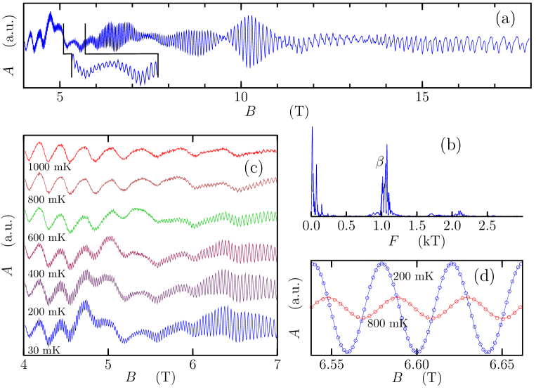
Figure 2: Typical quantum oscillations from PrOs₄Sb₁₂. (a) shows data from 18 T to 4 T. (b) shows the Fourier spectrum of the trace in (a), after the data have been replotted as a function of $1/B$. The $\beta$ frequency corresponds to the broad peak above 1 kT. (c) shows data from 4 to 7 T, between 30 mK and 1 K, to illustrate the temperature dependence of the oscillation amplitudes. (d) shows the results of fitting Eq. (3) to narrow sections of the data at 6.6 T. Note that there is a phase shift between the 200 mK and 800 mK oscillations. The data in (d) have been filtered so that only frequencies between 0.5 and 1.5 kT are present. The solid lines are the fitted curves.

Normally, a Fourier spectrum such as Fig. 2b consists of sharp peaks arising from well-defined extremal areas of the Fermi surface, and, indeed, sharp peaks corresponding to the low frequency oscillation of Fig 2a can be seen below 0.3 kT. The $\beta$ peak, however, is a broad clump of peaks. This is not due to a superposition of many frequency components, but, as we shall show, is because the Fermi surface area is changing non-linearly, and by a large amount as the magnetic field is swept. As a result, Fourier analysis is not a useful way of analyzing the $\beta$ oscillations in PrOs₄Sb₁₂. Instead, we have adopted the simple procedure of fitting the oscillations over narrow magnetic field ranges, just three periods wide, with a function of the form

$$A_{f}\sin\left(2\pi F_{f}/B+\phi_{f}\right),$$ (3)

which is based on the Lifshitz-Kosevich expression (1). $A_{f}$, $F_{f}$ and $\phi_{f}$ are the fitted dHvA amplitude, frequency and phase. Fig. 2d shows an example of such fits to sections of the data centred on 6.6 T, at 200 and 800 mK.

This fitting procedure allows us to extract the field and temperature dependence of the dHvA frequency. Figure 3a shows the $B$ dependence of $F_{f}$ at 100, 400, 700 and 1200 mK. In this figure, the arrows indicate the approximate boundaries of the AFQ phase according to reference Tayama et al. (2003). (Note that 1200 mK is above the maximum AFQ phase transition temperature.) In the 100 mK data of Fig. 3a (orange triangles) it can be seen that $F_{f}$ jumps up upon entry into the AFQ phase, and jumps down upon exiting the phase near 12 T, establishing that the Fermi surface is sensitive to the AFQ order.

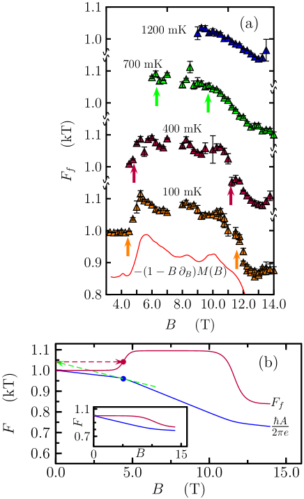
Figure 3: The magnetic field dependence of the dHvA frequency. (a) dHvA frequency $F_{f}$ vs. $B$ at temperatures from 100 mK to 1.2 K. The values of $F_{f}$ are extracted from fits of Eq. 3 to sets of three periods, as described in the text. The arrows indicate the boundaries of the AFQ phase Tayama et al. (2003). The absence of low-field data at high temperature is due to the dHvA thermal damping factor in the Lifshitz-Kosevich amplitude, Eq.  2. The red curve at the bottom is proportional to $-(1-B\frac{\partial}{\partial B})M$, where $M$ is the magnetization derived from the 60 mK $M$ vs. $B$ data of reference Tayama et al. (2003). (b) Main figure: simple model curves showing a hypothetical low-temperature field dependence of the Fermi surface area ${\cal A}$ (blue line) together with the back-projected frequency $F_{f}$ that would be seen in quantum oscillation measurements (red line). The dashed green line shows how $F=\hbar{\cal A}/2\pi e$ at 4.4 T is back-projected to produce the measured frequency $F_{f}$ (red dot). The inset shows a hypothetical field dependence of $\hbar{\cal A}/2\pi e$ and the corresponding measured dHvA frequency $F_{f}$ at a temperature above the maxiumum AFQ phase transition temperature. The hypothetical field dependences of ${\cal A}$ were chosen to produce $F_{f}$ curves that resemble the measured curves in (a) at 100 mK and 1200 mK.

When an extremal area of the Fermi surface is magnetic field dependent, the measured dHvA frequency cannot be interpreted using the Onsager formula, $F=\hbar{\cal A}/2\pi e$ (as explained in Appendix 1). Instead, the measured frequency is the ‘back-projection’ of $F$, given by $F_{f}=(1-B\partial/\partial B)F$. Geometrically, $F_{f}$ is the intercept at $B=0$ of the tangent to $F$, illustrated in Fig. 3b for the point at 4.4 T (blue dot), which back-projects along the dashed green line, to give the value of $F_{f}$ shown by the red dot on the upper curve.

Thus, rather than the Fermi surface expanding and contracting at the AFQ phase boundaries, as the 100 mK data in Fig. 3a would imply if the Onsager formula $F=\hbar{\cal A}/2\pi e$ were applied, we believe that it follows something like the blue curve in the main panel of Fig. 3b: the Fermi surface contracts monotonically with increasing field, but it does so more rapidly within the AFQ phase, producing a a back-projected frequency (red line) that jumps up upon entering the AFQ phase.

At the bottom of Fig. 3b, below the 100 mK data, is a red curve showing the behaviour of $-(1-B\partial/\partial B)M(B)$, where $M(B)$ is taken from published magnetisation measurements at 60 mK Tayama et al. (2003). At high field and low temperature $M(B)$ measures the average occupancy of the $\Gamma_{4}^{(2),+}$ crystal field state, because $\Gamma_{4}^{(2),+}$ has a magnetic moment while $\Gamma_{1}$ does not. The close correspondence between $-(1-B\partial/\partial B)M(B)$ at 60 mK and our $F_{f}(B)$ data at 100 mK strongly suggests that ${\cal A}(B)$ is proportional to $-M(B)$ (or more precisely, the change in ${\cal A}(B)$, ${\cal A}(B)-{\cal A}(0)$, is proportional to $-M(B)$). This, in turn, tells us that ${\cal A}(B)$ is also dependent on the occupancy of $\Gamma_{4}^{(2),+}$. Our main conclusion from Fig. 3a is, therefore, that the $\beta$ sheet of the Fermi surface shrinks as the occupancy of $\Gamma_{4}^{(2),+}$ grows relative to that of $\Gamma_{1}$.

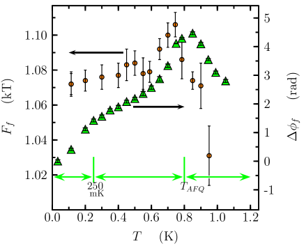
Figure 4: Temperature dependence at 6.2 T of the dHvA frequency $F_{f}$ (circles) and the phase $\Delta\phi_{f}(T)$ (green triangles). Both show a peak near the antiferroquadrupolar phase transition, $T_{AFQ}$ (taken from reference Tayama et al. (2003)), but the phase data are less noisy, and they reveal an additional downturn below $\sim$ 250 mK that is not evident in the backprojected frequency $F_{f}$.

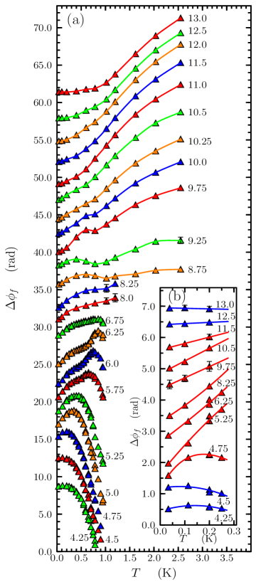
Figure 5: The temperature dependence of $\Delta\phi_{f}(T)$ at magnetic fields spanning the AFQ phase. Because of the dHvA thermal damping factor (see Eq. 2), below 8 T we only have data up to 950 mK. Error bars are statistical errors from averaging several sweeps with identical conditions. Where errors are not plotted, the error bars are smaller than the point size. The lines are guides to the eye, and the curves are shifted vertically for clarity; without this shift the lowest temperature point would be at 0 radians for every curve. The inset, (b), focuses on data below 300 mK for selected curves from (a). The blue(red) data are outside(inside) the AFQ phase. The lines are guides to the eye.

We turn now to the temperature dependence of the Fermi surface, which is the primary focus of this paper. In Figure 4, the small circles show the temperature dependence of $F_{f}$ at 6.2 T. At this field, the thermally driven AFQ phase transition, $T_{AFQ}$, is near 0.8 K. There is a peak in $F_{f}(T)$ near this temperature, but the error bars are large, the data are rather noisy, and it is not simple to connect the temperature dependence of the back-projected frequency to the temperature dependence of the Fermi surface.

The triangles in Fig. 4 illustrate another approach to the data, in which we consider the temperature dependence of the dHvA phase. That the phase is temperature dependent can be seen in Fig. 2d: there is roughly a $\pi/2$ phase shift between 200 mK and 800 mK. We extract this phase shift from the data by fitting Eq. 3 to three periods surrounding the field of interest (6.2 T for the data in Fig. 4) at the base temperature of our measurement, $T_{\circ}$, using $A_{f}$, $F_{f}$ and $\phi_{F}$ as free parameters. This fit yields $A_{f}(T_{\circ})$, $F_{f}(T_{\circ})$ and $\phi_{F}(T_{\circ})$. At all higher temperatures ($T>T_{\circ}$), $F_{f}$ is held fixed at its base temperature value, $F_{f}(T_{\circ})$, and only $A_{f}(T)$ and $\phi_{f}(T)$ are free parameters in the fits. The temperature dependent phase shift is then

$$\Delta\phi_{f}(T)=\phi_{f}(T)-\phi_{f}(T_{\circ}).$$ (4)

Fig. 4 shows that $\Delta\phi_{f}(T)$ is less noisy than $F_{f}(T)$, with error bars that are smaller than the data points, and with a clear peak near $T_{AFQ}$.

The interpretation of $\Delta\phi_{f}(T)$ is straightforward:Lonzarich and Gold (1974) If the temperature-dependent change of $\cal A$ is small compared to $\cal A$ itself then, at a given field $B_{\circ}$,

$$\Delta\phi_{f}(T,B_{\circ})=\frac{\hbar}{eB_{\circ}}\,\Delta{\cal A}(T,B_{\circ}).$$ (5)

That is, the temperature dependent phase shift directly gives the temperature dependent change of the Fermi surface extremal area. This is shown in Appendix 1. In particular, unlike $F_{f}(T)$, $\Delta\phi_{f}(T)$ does not depend on the field-derivative of ${\cal A}$. Thus $\Delta\phi_{f}(T)$ is easier to interpret than $F_{f}(T)$: when $\Delta\phi_{f}$ increases, the Fermi surface is expanding, and vice-versa.

In Fig. 5, we plot $\Delta\phi_{f}(T)$ at several magnetic fields spanning the AFQ phase, finding large, systematic and often non-monotonic temperature dependence. According to our intepretation of the $F_{f}(B)$ data in Fig. 3, these changes reflect the relative occupancies of $\Gamma_{1}$ and $\Gamma_{4}^{(2),+}$.

IV Discussion

It is important to emphasize that, although the changes we observe in ${\cal A}(T,B)$ are proportional to changes in $-M(T,B)$, the magnetization is not causing the changes in ${\cal A}$. What we see as a single quantum oscillation frequency is actually the superposition of oscillations from spin-up and spin-down branches of the Fermi surface, which have very nearly the same back-projected oscillation frequency Shoenberg (1984). Changing the polarized magnetic moment on the localized $4f$ states will produce a contribution to the spin splitting of these branches of the Fermi surface, additional to the Pauli paramagnetic spin splitting that the applied magnetic field alone would produce. However, it will not change their average back-projected dHvA frequency, which is what we observe. The field and temperature dependence of ${\cal A}(B,T)$ must primarily reflect changes in the charge distribution on the Pr $f$-orbital as the relative occupation of $\Gamma_{1}$ and $\Gamma_{4}^{(2)}$ changes. This is important because it means that, even if the crystal field levels were both non-magnetic singlets, the Fermi volume measurement would still be sensitive to changes in their occupancy, although the magnetisation $M$ would not.

If we examine the temperature dependence of $\Delta\phi_{f}(T)$ in Fig. 5, much of this behaviour can be easily understood within the existing model of the crystal field states of PrOs₄Sb₁₂, when we consider that the $\beta$-sheet expands when the occupancy of $\Gamma_{1}$ increases at the expense of $\Gamma_{4}^{(2),+}$, and vice-versa. Thus, for magnetic fields below the lower boundary of the AFQ phase (at 4.25 T, for example) $\Delta\phi_{f}$ decreases monotonically (the $\beta$ Fermi surface contracts) with increasing $T$ because the $\Gamma_{4}^{(2),+}$ state is becoming thermally occupied at the expense of the $\Gamma_{1}$ ground state. For fields above the upper boundary of the AFQ phase (e.g. 13 T) we see the opposite behaviour because the relative positions of $\Gamma_{1}$ and $\Gamma_{4}^{(2),+}$ are now reversed: $\Delta\phi_{f}$ increases monotonically (the $\beta$ Fermi surface expands) with increasing $T$ because Pr $4f$ electrons are being thermally excited from the $\Gamma_{4}^{(2),+}$ ground state to the $\Gamma_{1}$ excited state.

For magnetic fields corresponding to the AFQ region, the behaviour of $\Delta\phi_{f}(T)$ is more complicated, but we assume that it still reflects the relative occupations of the crystal field states as we have described. For $4.7~{}T\lesssim B\lesssim 8.5~{}T$ there is a maximum in $\Delta\phi_{f}(T)$ at the AFQ thermal phase boundary $T_{AFQ}$. This is clearly seen in Fig. 4, as well as in several curves in Fig. 5. As noted in the introduction, AFQ order involves a superposition at each Pr site of the form $\sum_{j}a_{i,j}(B,T)\,|\Gamma_{4}^{(2),j}\rangle+b_{i}(B,T)\,|\Gamma_{1}\rangle$, where $i=1,2$ indexes the AFQ sublattice and $j=+,0,-$ indexes the triplet crystal-field sublevels (see Appendix 2). As the temperature increases in this field and temperature range, the amplitude of the AFQ order parameter decreases. This is reflected in a decrease in the $a_{i,j}(B,T)$ and a corresponding increase in $b_{i}(B,T)$: $\Gamma_{4}^{(2),+}$ is higher in energy than $\Gamma_{1}$, so its incorporation into the ground state costs crystal field energy that can only be compensated by AFQ energy. Thus, as $T$ increases towards $T_{AFQ}$, the occupancy of $\Gamma_{1}$ increases at the expense of $\Gamma_{4}^{(2)}$, and the $\beta$ Fermi surface expands. For $T>T_{AFQ}$, AFQ order is gone, and there is an incoherent, thermal superposition of the crystal field states on the Pr sites. The occupation of $\Gamma_{1}$ therefore falls while that of $\Gamma_{4}^{(2),+}$ rises, as Pr 4f electrons are thermally excited into the $\Gamma_{4}^{(2),+}$ state causing the $\beta$ Fermi surface to shrink and $\Delta\phi_{f}(T)$ to fall. The non-monotonic behaviour of $\Delta\phi_{f}(T)$ thus reflects a change in regime from coherent superposition to incoherent thermal occupation of crystal field states.

For $8.5~{}T\lesssim B\lesssim 11.6~{}T$, we would expect this situation to be reversed due to the crystal field level-crossing, producing a minimum in $\Delta\phi_{f}(T)$ at $T_{AFQ}$. This minimum is observed up to 9.75 T, but above this field we see $\Delta\phi_{f}$, and therefore $\Gamma_{1}$ occupancy, monotonically increasing with increasing $T$ at all temperatures, even within the AFQ phase. We do not fully understand this behaviour, but it appears to signal a change in the AFQ ground state in this field region, perhaps to an admixture of the different $\Gamma_{4}^{(2)}$ states with very little $\Gamma_{1}$, consistent with previous suggestions that the ordered structure changes at a first-order phase transition within the AFQ phase (shown as the higher-field purple line in Fig. 1)Tayama et al. (2003).

Temperature dependence of Fermi surface areas is a subject that has only rarely been discussed with respect to quantum oscillations Lonzarich and Gold (1974); Yelland and Hayden (2007); Shoenberg (1984), and such a strongly temperature dependent phase, particularly a non-monotonic variation of $\Delta\phi_{f}(T)$, has not to our knowledge been previously reported. This does not mean that temperature dependence of the Fermi surface is uncommon, but the usual way of analysing dHvA oscillations using Fourier transforms could cause such temperature dependent phases to have gone unnoticed. Application of Eq. 5 to the data in Fig. 5 illustrates how sensitive the dHvA phase is to variations in Fermi surface area: a tiny change in ${\cal A}$ leads to a large change in $\phi_{f}$. At 10 T, for example, $\Delta\phi_{f}$ reaches about 11 radians at 2.5 K, which corresponds to a change in ${\cal A}$ of only $\sim 2$%.

The high sensitivity of the dHvA technique, particularly at millikelvin temperatures, has allowed us to observe some unexpected behaviour in the $T\rightarrow 0$ K limit. Figure 5b shows that there is a clear difference between data outside the AFQ phase (at 4.25 T, 4.5 T, 12.5 T and 13.0 T), in which $\Delta\phi_{f}(T)$ approaches $T=0$ K with zero slope, and data within the AFQ phase, which show a distinctly positive slope as $T\rightarrow 0$ K. We have found similar behaviour with the magnetic field parallel to the (100) direction (data not shown). The sign of the $T\rightarrow 0$ slope is positive everywhere within the AFQ phase, independent of whether the magnetic field is higher or lower than the singlet-triplet level crossing near 8 T. The change in the slope of $\Delta\phi_{f}(T)$ at low temperature can be seen very clearly in Fig. 4, setting in near 250 mK.

In a mean-field picture, the AFQ order parameter should saturate as $T\rightarrow 0$ K, so the naive expectation is that the occupancy of $\Gamma_{1}$ and $\Gamma_{4}^{(2)}$ should stop changing with temperature. In terms of AFQ order, $\phi_{f}(T)$ should, therefore, have a slope that goes to zero for $T\ll T_{AFQ}$, rather than a slope that increases, as we observe. Although the behaviour we observe is not expected, a hint as to its origin can be found in thermal expansion measurements, which also showed temperature dependence for $T\ll T_{AFQ}$, a result that was ascribed to the nuclear hyperfine interaction Oeschler et al. (2004).

The nuclear hyperfine interaction normally has a negligible effect on crystal field levels, but is enhanced in Pr compounds with singlet ground states Jensen and Mackintosh (1991). Pr has one stable isotope, with a $J=5/2$ nucleus, so what we have been calling “the ground state” is actually a manifold of six hyperfine states, split primarily by the hyperfine dipole interaction $H_{HF}=AI\cdot J=AI_{z}J_{z}+(I_{+}J_{-}+I_{-}J_{+})/2$, with $A\sim 50$ mK Aoki et al. (2002b). The $I_{z}J_{z}$ term, and the fact that $J_{z}=0$ for $\Gamma_{1}$, means that the hyperfine splitting will be proportional to the amount of $\Gamma_{4}^{(2),+}$ in the electronic ground state. A key point, however, is that the off-diagonal $I_{+}J_{-}$ and $I_{-}J_{+}$ terms mix $\Gamma_{4}^{(2),+}$ and $\Gamma_{1}$, so that, within the hyperfine manifold, different states can have differing weights of $\Gamma_{4}^{(2),+}$ and $\Gamma_{1}$, with the hyperfine ground state expected to have the most $\Gamma_{4}^{(2),+}$. Outside the AFQ phase this mixing is weak because $\Gamma_{1}$ and $\Gamma_{4}^{(2),+}$ are separated in energy, so the perturbation is second order in $AI_{+}J_{-}$. Within the AFQ phase, however, the ground state is a superposition of $\Gamma_{1}$ and $\Gamma_{4}^{(2)}$, so there is a first-order matrix element and the mixing is much stronger, i.e. it is proportional to $A$, rather than $A^{2}$.

Within this picture, the low temperature contraction of the $\beta$ Fermi surface within the AFQ phase can be understood: for temperatures above about 300 mK, all of the hyperfine states of the ground state manifold are equally thermally populated, but as $T$ falls towards 0 K the lower hyperfine states, which have more $\Gamma_{4}^{(2),+}$ character, become preferentially occupied. Because the $\beta$ Fermi surface ‘doesn’t like’ $\Gamma_{4}^{(2)}$, (as we have discussed above) it shrinks. In Appendix 2 we present a toy model that illustrates and supports this interpretation.

The observed effect on the Fermi surface is only of the order of 0.08% of ${\cal A}$, but is still easily observed by quantum oscillations: At several magnetic field values, the hyperfine interaction is actually a stronger influence on the admixture of $\Gamma_{1}$ and $\Gamma_{4}^{(2),+}$ than the AFQ order.

We note that the hyperfine interaction may have a profound effect on the phase transition line at the quantum critical point marking the lower boundary of the AFQ phase, since hyperfine mixing should stabilize the AFQ order. Thus we would expect that the phase line could show deviations from the predictions of simple AFQ theory in the low mK temperature range. There may also be enhanced nuclear adiabatic demagnetization effects on crossing the AFQ phase boundary.

We are not aware of any other technique that can so sensitively detect changes in electronic states in this low temperature regime, although similar conclusions could perhaps be drawn from similarly detailed thermal expansion measurements, if they were performed. We note that the exact energy splitting of the hyperfine levels will be very sensitive to the electronic states that form the hidden order in a multipolar system, so it may be possible, by detailed fitting of the temperature dependence, to test models of hidden order electronic states. This is an interesting possibility in other hidden order systems.

V Conclusions

In conclusion, we have observed a qualitatively new effect in quantum oscillations, which arises from the temperature dependent expansion and contraction of a Fermi surface as the population of localized electronic states changes. This very sensitive method of measuring the temperature dependence of the Fermi volume has allowed us to map the relative occupation of crystal field levels in PrOs₄Sb₁₂, including the change from Boltzmann-type thermal occupation to the coherent superposition of crystal field levels that signals AFQ order in this material. It has also allowed us to observe new features of the hyperfine interaction in PrOs₄Sb₁₂, related to a jump in the hyperfine mixing of the crystal field levels on entry into the AFQ phase. This application of quantum oscillations may, in future, give useful information about the nature of hidden order in other systems.

Acknowledgements:

We are grateful to John Sipe for helpful discussions. This research was funded by the National Science and Engineering Council of Canada, the Canadian Institue for Advanced Research, the Marie Curie Program of the European Science Foundation, and the U.S. Department of Energy, Office of Basic Energy Sciences, DE-FG02-99ER45748.

Appendix 1: The effect of a field and temperature dependent Fermi volume on quantum oscillations

If the extremal area ${\cal A}$ of a Fermi surface is field or temperature dependent, it will affect the quantum oscillations through the Onsager expression

$$F=\frac{\hbar{\cal A}}{2\pi e},$$ (6)

where $F$ is the dHvA frequency appearing in the argument of the oscillatory term, $\sin(2\pi F/B+\phi_{\circ})$ (see Eq. 1). Because $F$ appears in combination with $1/B$, it cannot be extracted from the observed quantum oscillation frequency Van Ruitenbeek et al. (1982). To see this, consider a field sweep centered on a field $B_{\circ}$, and expand ${\cal A}(B,T)$ to first order in $\delta B$:

$$\hbar\frac{{\cal A}(B,T)}{eB}+\phi_{\circ}\simeq$$

$$\hbar\frac{{\cal A}(B_{\circ},T)+(B-B_{\circ})\partial_{B}{\cal A}(B,T)|_{B_{\circ}}}{eB}+\phi_{\circ}=$$

$$\hbar\frac{{\cal A}(B_{\circ},T)-B_{\circ}\partial_{B}{\cal A}(B,T)|_{B_{\circ}}}{eB}+\frac{\hbar}{e}\frac{\partial{\cal A}(B,T)}{\partial B}|_{B_{\circ}}+\phi_{\circ}$$

$$\equiv 2\pi\frac{F_{f}(B_{\circ},T)}{B}+\phi^{\prime}_{\circ}(B_{\circ},T),$$ (8)

where we have used the shorthand notation $\partial_{B}\equiv\partial/\partial B$. The frequency

$$F_{f}(B_{\circ})\equiv\left(1-B\frac{\partial}{\partial B}\right)\frac{\hbar{\cal A}}{2\pi e}$$ (9)

is called the “back-projected” frequency, and it is the frequency that is observed in a quantum oscillation measurement.

Geometrically, the back-projected frequency is the intercept of the tangent of $F(B)$ at $B=0$, as illustrated in the main panel of Fig. 3b. The blue curve gives a possible field dependence of the Fermi surface cross-sectional area: we hypothesize that the $\beta$ Fermi surface shrinks continuously with increasing field, but the slope is more negative within the AFQ region. Back-projection is shown for one point, at 4.4 T. The green dashed line is the tangent of $F(B)$ at that field, and its intercept at $B=0$ gives $F_{f}$. In this model, the reason that $F_{f}$ jumps up when the AFQ phase is entered is not because ${\cal A}$ itself changes suddenly, but rather because its slope changes suddenly, causing the back-projection to jump. This hypothesis is supported by the field-dependence of the magnetization, which looks similar to the blue curve (but with a positive slope) Tayama et al. (2003). In particular, we note the striking correspondence between $F_{f}$ at 100 mK and the red curve below it in Fig. 3a, which is proportional to $-(1-B\partial/\partial B)M(B)$. As noted in the text, this correspondence strongly suggests that ${\cal A}(B)-{\cal A}(0)$ is proportional to $-M(B)$.

Temperature Dependent Fermi Volume

If an extremal area ${\cal A}$ of a Fermi surface is temperature dependent, the most useful analysis of quantum oscillations is to examine the temperature dependence of the dHvA phase. It initially seems more promising to extract $F_{f}(T)$ at each temperature by fitting

$$A_{f}(T)\sin\left(2\pi\frac{F_{f}(T)}{B}+\phi_{f}(T)\right)$$ (10)

where $A_{f}(T)$, $F_{f}(T)$ and $\phi_{f}(T)$ are free parameters representing the amplitude, frequency and phase of the oscillation. However, in the case of PrOs₄Sb₁₂, the rapid field dependence of the Fermi surface in some regions (e.g. at the boundaries of the AFQ phase) led us to restrict our analysis to very narrow field ranges, and fitting the frequency of only a few oscillations is inherently noisy, as can be seen in Fig. 4. Moreover, from Eq. 9 above, $F_{f}(T)$ gives a combination of the temperature dependence of $\cal A$ and its derivative with respect to field, which is difficult, if not impossible, to deconvolve to arrive at the temperature dependence of ${\cal A}$. If we instead fix $F_{f}$ at the value obtained by fitting the oscillations in the lowest-temperature trace, allowing only $A_{f}(T)$ and $\phi_{f}(T)$ to be free parameters at higher temperatures, i.e. fitting

$$A_{f}(T)\sin\left(2\pi\frac{F_{f,\circ}}{B}+\phi_{f}(T)\right)$$ (11)

to the $T>T_{\circ}$ data, where $F_{f,\circ}=F_{f}(B_{\circ},T_{\circ})$ and $T_{\circ}$ is base temperature, this produces much less noisy results (see Fig. 4). This approach has also been taken in some previous dHvA studies Lonzarich and Gold (1974); Yelland and Hayden (2007).

The interpretation of the temperature dependent phase turns out to be surprisingly simple. Assume that the change in ${\cal A}$ at temperature $T$ relative to its value at base temperature, $\Delta{\cal A}(T)\equiv{\cal A}(T)-{\cal A}(T_{\circ}),$ is small compared with ${\cal A}(T)$ itself (in our case the ratio is less than about 2%). Then, showing the field dependence explicitly so that the back-projection can be included at the appropriate time, we write

$$\hbar\frac{{\cal A}(B,T)}{eB}+\phi_{\circ}=\hbar\frac{{\cal A}(B,T_{\circ})+\Delta{\cal A}(B,T)}{eB}+\phi_{\circ}$$ (12)

$$\simeq \hbar\frac{{\cal A}(B,T_{\circ})}{eB}+\hbar\frac{\Delta{\cal A}(B_{\circ},T)}{eB_{\circ}}+\phi_{\circ}$$

$$\simeq 2\pi\frac{F_{f}(B_{\circ},T_{\circ})}{B}+\hbar\frac{\Delta{\cal A}(B_{\circ},T)}{eB_{\circ}}+\phi^{\prime}(B_{\circ},T_{\circ}).$$ (13)

That is, a small correction to the frequency of an oscillation can, over a range of a few periods, be accurately be treated as a phase shift

$$\Delta\phi_{f}(B_{\circ},T)=\hbar\frac{\Delta{\cal A}(B_{\circ},T)}{eB_{\circ}},$$ (14)

where $\Delta\phi_{f}(B_{\circ},T)\equiv\phi_{f}(B_{\circ},T)-\phi_{f}(B_{\circ},T_{\circ})$. So the temperature dependent term in the phase directly gives the temperature dependence of the extremal area, with no contamination by the derivative. Note, however, that due to back-projection we do not know the value of ${\cal A}$ at $T_{\circ}$: we know quite precisely by how much ${\cal A}$ changes with temperature, but we know much less precisely the absolute value of ${\cal A}$, at a given field.

Appendix 2: Interaction between hyperfine coupling and quadrupolar order

Our dHvA results for PrOs₄Sb₁₂ clearly show a downturn in $\Delta\phi_{f}(T)$ as $T\rightarrow 0~{}K$ within the AFQ phase. For example, at $T\simeq 250$ mK in Fig. 4 (green triangles), and similarly in several curves in Fig. 5. The inset of Fig. 5 shows that the increased low-temperature slope is confined to the AFQ phase. In this Appendix we describe a toy model of the coupling between the dipolar hyperfine interaction and quadrupolar order that could explain this behaviour. The model is somewhat artificial because it ignores the broadening of the crystal-field states by nearest-neighbour interactions, and because we have put the AFQ order in by hand.

We use as our basis states ($\Gamma_{1}$, $\Gamma_{4}^{(2),+}$, $\Gamma_{4}^{(2),0}$, $\Gamma_{4}^{(2),-}$). In this basis, the crystal-field Hamiltonian in the presence of a magnetic field can be written Shiina (2004)

$${\cal H}_{cf}=\left(\begin{array}[]{cccc}0&0&-\delta h&0\\ 0&\Delta-h&0&0\\ -\delta h&0&\Delta&0\\ 0&0&0&\Delta+h\end{array}\right).$$ (19)

We have used the notation of Shiina and Aoki Shiina and Aoki (2004), where $h=g\mu_{B}\alpha H$ is the coupling of the $+$ and $-$ triplet states to the applied field, $\delta=\beta/\alpha$ is a field-dependent off-diagonal coupling between the singlet $\Gamma_{1}$ and the $\Gamma_{4}^{(2),0}$ member of the triplet, and $\Delta$ is the crystal field splitting between the singlet and the triplet at zero field. The parameters $\alpha$ and $\beta$ are $\alpha=5/2-2d^{2}$ and $\beta=2\sqrt{5/3}d$, where non-zero $d$ arises from the reduction of the symmetry of the Pr site from octahedral to tetrahedral, and characterizes the resulting mixing of $\Gamma_{5}$ and $\Gamma_{4}$ triplets that would be crystal field eigenstates in pure octahedral symmetry. The eigenvalues of this Hamiltonian are shown by the dashed red lines in Fig. 6a. (This Hamiltonian may not be complete – magnetoresistance measurements on dilute Pr_1-xLa_xOs₄Sb₁₂ suggest that the crystal-field level crossing is avoided even in the absence of quadrupolar order Rotundu et al. (2007).)

To this we artificially add quadrupolar order between 4.75 and 11.5 T. We choose the so-called $X_{y}$ form of quadrupolar order (see e.g. ref. Kusunose et al. (2009)):

$${\cal H}_{Q}=\frac{1}{c1^{2}+c2^{2}}\left(\begin{array}[]{cccc}0&c1&0&c1\\ c1&0&c2&0\\ 0&c2&0&-c2\\ c1&0&-c2&0\end{array}\right),$$ (24)

where we put in the AFQ order by hand by setting

$$c1 = \left\{\begin{array}[]{ll}c1_{0}(h-\frac{\Delta}{2.0})(\frac{3.5\Delta}{2.0}-h)&{\rm if}\frac{\Delta}{2.0}<h<\frac{3.5\Delta}{2.0}\\ 0&{\rm otherwise}\end{array}\right.$$ (27)

where $c1_{0}=0.04\sqrt{35.0(1-d^{2})}$ and $c2=0.01\sqrt{3}(13-20d^{2})c1/c1_{0}$. Between 4.75 and 11.5 T this term mixes the $\Gamma_{1}$ and the $\Gamma_{4}^{(2)}$ states, and removes the $\Gamma_{1}/\Gamma_{4}^{(2),+}$ level crossing.

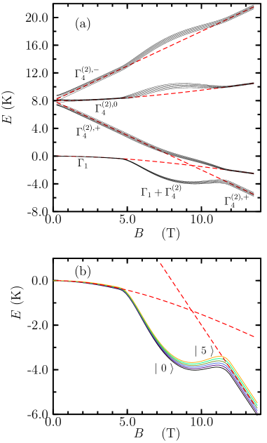
Figure 6: Energy levels and eigenstates for the two lowest crystal field levels of PrOs₄Sb₁₂ in the presence of a magnetic field, wth quadrupolar and hyperfine couplings. (a) Energy vs. field. The red dashed lines are the states of Eq. 19 with no quadrupolar order and the hyperfine interaction turned off. The $-\delta h$ term mixes $\Gamma_{4}^{(2),0}$ with $\Gamma_{1}$ so its energy is field dependent, despite $\Gamma_{1}$ being a singlet. Turning on quadrupolar order (Eq. 24) between 4.75 and 11.5 T avoids the level crossing of $\Gamma_{4}^{(2),+}$ and $\Gamma_{1}$, and makes the ground state an admixture of $\Gamma_{1}$ and $\Gamma_{4}^{(2)}$ in this field range. The hyperfine Hamiltonian (Eq. 27) lifts the degeneracy of the six hyperfine eigenstates. (b) The ground state manifold of figure (a). The black line is the lowest hyperfine state, labelled $|0\rangle$, while the yellow line is the highest, labelled $|5\rangle$.

When we introduce the hyperfine dipole interaction the Hamiltonian expands to a 24 $\times$ 24 matrix, with additional matrix elements of

$${\cal H}_{HF}=A\vec{I}\cdot\vec{J}=AI_{z}J_{z}+\frac{A}{2}\left(I_{+}J_{-}+I_{-}J_{+}\right).$$

Diagonalizing the full Hamiltonian (including crystal field, quadrupolar and hyperfine terms) gives the black lines in Fig. 6a. Each of the electronic energy levels is split into six hyperfine levels. Fig. 6b focuses on the ground state manifold, and it can be seen that the hyperfine splitting grows rapidly through the AFQ region as the triplet $\Gamma_{4}^{(2),+}$ is progressively mixed into the ground state manifold by the AFQ order. In effect, at a given magnetic field, the AFQ Hamiltonian produces a certain admixture of $\Gamma_{1}$ and $\Gamma_{4}^{(2),+}$ in the ground state. The more $\Gamma_{4}^{(2)}$ there is in the ground state, the larger the dipole term in the hyperfine Hamiltonian, and thus the larger the splitting of the hyperfine states. However the hyperfine Hamiltonian, even though it is weak, has a back-effect on the states through the $I_{+}J_{-}$ and $I_{-}J_{+}$ terms, modifying the admixture of $\Gamma_{1}$ and $\Gamma_{4}^{(2),+}$ within the various hyperfine states of the ground-state manifold. Fig. 7a shows the result: the six hyperfine states in the ground-state manifold have different amounts of $\Gamma_{4}^{(2)}$ character, with the lowest state, $|0\rangle$, having up to about 5% more $\Gamma_{4}^{(2)}$ at a given field than the highest hyperfine state $|5\rangle$. As a result of these differing amounts of $\Gamma_{4}^{(2)}$, when the temperature becomes low enough that the lower hyperfine states are preferentially occupied, the occupancy of $\Gamma_{4}^{(2),+}$ increases, causing the $\beta$ sheet of the Fermi surface to shrink.

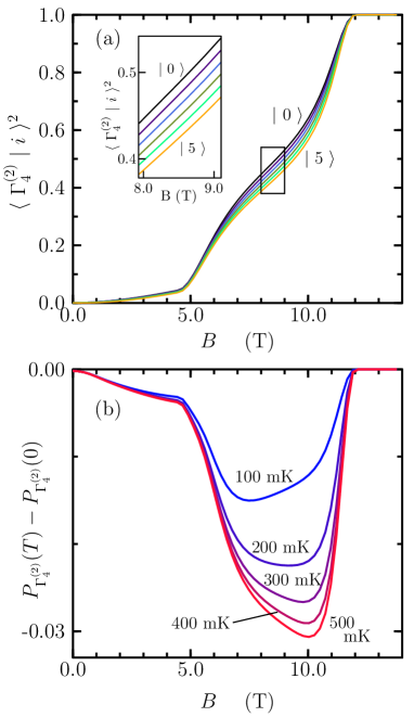
Figure 7: (a) The proportion of $\Gamma_{4}^{(2)}$ in the six hyperfine states of the ground state manifold. At $B=0$ all of the hyperfine levels in the electronic ground state are purely $\Gamma_{1}$. At $B>11.75$ T, they are all purely $\Gamma_{4}^{(2)}$. In the AFQ region their composition is surprisingly different: at a given field, the ground state, $|0\rangle$ has the most $\Gamma_{4}^{(2)}$ character, and each successive excited hyperfine state has progressively less. The inset zooms in on the curves between 8 and 9 T. (b) Change in thermal occupation of $\Gamma_{4}^{(2)}$ from its $T=0$ value, calculated by applying a Boltzmann distribution to the eigenstates in (c). In the AFQ region, occupation of $\Gamma_{4}^{(2)}$ falls with increasing $T$ because the excited hyperfine states, which have less $\Gamma_{4}^{(2)}$ character, become thermally occupied.

In Fig. 7b, a Boltzmann average of the occupancy of $\Gamma_{4}^{(2)}$ over the ground state manifold, at selected temperatures, allows us to plot the change in $\Gamma_{4}^{(2)}$ occupancy relative to $T=0$ K as a function of $B$. It can be seen that the change of $\Gamma_{4}^{(2)}$ occupancy with temperature is much stronger within the AFQ phase. Moreover, it changes in the same direction as suggested by our data (decreasing weight of $\Gamma_{4}^{(2),}$ with increasing temperature). The largest change occurs between 0 K and 100 mK, and the rate of change slows and becomes quite small between 400 mK and 500 mK. This is quite similar to our observations, and leads us to believe that a more rigorous model would provide good agreement. It also appears that a similar effect should be observed at temperatures well below 100 mK for fields below 4.75 T. Above the AFQ phase, however, the ground state is purely $\Gamma_{4}^{(2),+}$, so there is no temperature dependent admixture in the ground state manifold in this region.

In this model, we have ignored the hyperfine quadrupole interaction, which is weaker than the dipole interaction, but could also produce an observable effect below 100 mK. Of course, the occupancies of the hyperfine states will eventually saturate, and the Fermi surface will become temperature independent, but, in PrOs₄Sb₁₂, this may not happen until low millikelvin temperatures are reached.

Dependence of Fermi volumes on hyperfine levels is an intriguing prospect for future investigations of the physics of strongly correlated electron systems. From dHvA measurement such as we have described here, it should be possible to extract detailed information about the coupling of nuclear states to electronic energy levels, and thus determine the nature of the electronic energy levels themselves.

Appendix 3: Comparison with thermal expansion measurements

An obvious question regarding our results is whether the temperature dependence that we have observed in the $\beta$ Fermi surface might arise from simple changes in electron density due to thermal expansion of the crystal.

In free electron theory, the Fermi surface area is related to the volume by

$${\cal A}=\pi k_{F}^{2}=\pi\left(\frac{3\pi^{2}N}{V}\right)^{2/3},$$ (28)

where $k_{F}$ is the Fermi wave-vector, and $N/V$ is the conduction electron density. Thus a change in sample volume of $\delta V$ will produce a corresponding change of Fermi surface area of

$$\frac{\delta{\cal A}}{\cal A}=-\frac{2}{3}\frac{\delta V}{V}.$$ (29)

From data in reference Oeschler et al. (2004), at 6T with the field along (100) the fractional volume change is around $2.0\times 10^{-6}$ between 0.2 and 1 K. The dHvA phase changes by about 3 radians between 0 and 1 K under the same magnetic field conditions. Using $\Delta A=eB\Delta\phi/\hbar$, and the Onsager relation, $F=\hbar{\cal A}/2\pi e$, we find that this translates to a fractional change of the extremal area of $\sim+3\times 10^{-3}$, which is three orders of magnitude larger than the effect we would predict using equation 29 and the data in reference Oeschler et al. (2004), and it has the wrong sign: rather than expanding, the Fermi surface should shrink as $V$ increases. So the Fermi surface area change that we observe does not arise from a simple change in electron density due to thermal expansion of the crystal.

References

- Shull et al. (1951) C. Shull, W. Strauser, and E. Wollan, Phys. Rev. 83, 333 (1951).
- Fradkin et al. (2010) E. Fradkin, S. A. Kivelson, M. J. Lawler, J. P. Eisenstein, and A. P. Mackenzie, in Annual Review of Condensed Matter Physics, edited by J. S. Langer (Annual Reviews, 2010) pp. 153–178.
- Joynt and Taillefer (2002) R. Joynt and L. Taillefer, Rev. Mod. Phys. 74, 235 (2002).
- Hanzawa and Kasuya (1984) K. Hanzawa and T. Kasuya, J. Phys. Soc. Jpn. 53, 1809 (1984).
- Yamauchi et al. (1999) H. Yamauchi, H. Onodera, K. Ohoyama, T. Onimaru, M. Kosaka, M. Ohashi, and Y. Yamaguchi, J. Phys. Soc. Jpn. 68, 2057 (1999).
- Morin and Schmitt (1990) P. Morin and D. Schmitt, “Handbook of ferromagnetic materials, vol. 5,” (Elsevier, Amsterdam, 1990) p. 1.
- Walker et al. (1994) M. B. Walker, C. Kappler, K. A. McEwen, U. Stegenberger, and K. N. Clausen, J. Phys. Cond. Mat. 6, 7365 (1994).
- Mydosh and Oppeneer (2011) J. A. Mydosh and P. M. Oppeneer, Rev. Mod. Phys. 83, 1301 (2011).
- Aoki et al. (2002a) Y. Aoki, T. Namiki, S. Ohsaki, S. R. Saha, H. Sugawara, and H. Sato, J. Phys. Soc. Jpn. 71, 2098 (2002a).
- Shiina (2004) R. Shiina, J. Phys. Soc. Jpn. 73, 2257 (2004).
- Kohgi et al. (2003) M. Kohgi, K. Iwasa, M. Nakajima, N. Metoki, S. Araki, N. Bernhoeft, J. Mignot, A. Gukasov, H. Sato, Y. Aoki, and H. Sugawara, J. Phys. Soc. Jpn. 72, 1002 (2003).
- Shiina and Aoki (2004) R. Shiina and Y. Aoki, J. Phys. Soc. Jpn. 73, 541 (2004).
- Tayama et al. (2003) T. Tayama, T. Sakakibara, H. Sugawara, Y. Aoki, and H. Sato, J. Phys. Soc. Jpn. 72, 1516 (2003).
- Kaneko et al. (2007) K. Kaneko, N. Metoki, R. Shiina, T. D. Matsuda, M. Kohgi, K. Kuwahara, and N. Bernhoeft, Phys. Rev. B 75, 094408 (2007).
- Sugawara et al. (2002) H. Sugawara, S. Osaki, S. R. Saha, Y. Aoki, H. Sato, Y. Inada, H. Shishido, R. Settai, Y. Onuki, H. Harima, and K. Oikawa, Phys. Rev. B 66, 220504 (2002).
- Shoenberg (1984) D. Shoenberg, Magnetic oscillation in metals (Cambridge University Press, Cambridge, 1984).
- Lonzarich and Gold (1974) G. G. Lonzarich and A. V. Gold, Can. J. Phys. 52, 694 (1974).
- Yelland and Hayden (2007) E. A. Yelland and S. M. Hayden, Phys. Rev. Lett. 99, 196405 (2007).
- Oeschler et al. (2004) N. Oeschler, P. Gegenwart, F. Weickert, I. Zerec, P. Thalmeier, F. Steglich, E. D. Bauer, N. A. Frederick, and M. B. Maple, Phys. Rev. B 69, 235108 (2004).
- Jensen and Mackintosh (1991) J. Jensen and A. R. Mackintosh, Rare Earth Magnetism (Clarendon Press, Berlin, 1991).
- Aoki et al. (2002b) Y. Aoki, T. Namiki, T. D. Matsuda, K. Abe, H. Sugawara, and H. Sato, Phys. Rev. B 65, 064446 (2002b).
- Van Ruitenbeek et al. (1982) J. M. Van Ruitenbeek, W. A. Verhoef, P. G. Mattocks, A. E. Dixon, A. P. J. Ven Deursen, and A. R. De Vroomen, J. Phys. F-Met. Phys. 12, 2919 (1982).
- Note (1) This can readily be verified by plotting together, for example, the functions , and with e.g. T, T and T, over the range .
- Rotundu et al. (2007) C. R. Rotundu, K. Ingersent, and B. Andraka, Phys. Rev. B 75, 104504 (2007).
- Kusunose et al. (2009) H. Kusunose, M. Matsumoto, and M. Koga, J. Phys. Soc. Jpn. 78, 094713 (2009).