A line confusion-limited millimeter survey of Orion KL

Abstract

Context. We present a study of the sulfur-bearing species detected in a line confusion-limited survey towards Orion KL performed with the IRAM 30-m telescope in the frequency range 80-281 GHz.

Aims. This study is part of an analysis of the line survey divided into families of molecules. Our aim is to derive accurate physical conditions, as well as molecular abundances, in the different components of Orion KL from observed SO and SO₂ lines.

Methods. As a starting point, we assumed LTE conditions obtain rotational temperatures. We then used a radiative transfer model, assuming either LVG or LTE excitation to derive column densities of these molecules in the different components of Orion KL.

Results. We have detected 68 lines of SO, ³⁴SO, ³³SO, and S¹⁸O and 653 lines of SO₂, ³⁴SO₂, ³³SO₂, SO¹⁸O, and SO₂ $\nu$₂=1. We provide column densities for all of them and also upper limits for the column densities of S¹⁷O, ³⁶SO, ³⁴S¹⁸O, SO¹⁷O, and ³⁴SO₂ $\nu$₂=1 and for several undetected sulfur-bearing species. In addition, we present 2$\arcmin$$\times$2$\arcmin$ maps around Orion IRc2 of SO₂ transitions with energies from 19 to 131 K and also maps with four transitions of SO, ³⁴SO, and ³⁴SO₂. We observe an elongation of the gas along the NE-SW direction. An unexpected emission peak appears at 20.5 km s^-1 in most lines of SO and SO₂. A study of the spatial distribution of this emission feature shows that it is a new component of a few arcseconds ($\sim$5$\arcsec$´´) in diameter, which lies $\sim$4$\arcsec$ west of IRc2. We suggest the emission from this feature is related to shocks associated to the $BN$ object.

Conclusions. The highest column densities for SO and SO₂ are found in the high-velocity plateau (a region dominated by shocks) and in the hot core. These values are up to three orders of magnitude higher than the results for the ridge components. We also find high column densities for their isotopologues in both components. Therefore, we conclude that SO and SO₂ are good tracers, not only of regions affected by shocks, but also of regions with warm dense gas (hot cores).

1 Introduction

The hot core phase of massive star formation shows a particularly rich chemistry that results from gas-phase chemical reactions and dust grain mantle evaporation. During cloud collapse, depletion of molecules onto dust surfaces takes place. When a new protostar forms, the surrounding gas and dust are heated and molecules sublimate from the grain mantles, giving rise to new species in the warm gas and to enhanced abundances of pre-existing species. The existence of molecular outflows and associated shocked regions also plays an important role in the chemical evolution, because they heat up the gas significantly and modify its chemistry.

Orion KL is the closest high-mass star-forming region ($\simeq$414 pc, Menten et al. 2007). It is one of the most studied regions owing its chemical complexity and high gas temperature, which lead to a dense and bright line spectrum. In the Orion KL cloud it is useful to differentiate five distinct components, characterized by different physical and chemical conditions (Blake et al. 1987, Persson et al. 2007, Tercero et al. 2010, and references therein): i) the hot core (HC) with 10$\arcsec$ diameter, which contains a high abundance of complex species (Wilson et al. 2000). It is characterized by line widths of 7$\leq$ $\Delta$v $\leq$ 15 km s^-1 at $v$_LSR $\simeq$ 5 km s^-1. It contains dense and warm gas with $T$_K$\simeq$200 K and $n$(H₂)$\simeq$10⁷ cm^-3. ii) The plateau (PL), a component with 30$\arcsec$ diameter, is affected by shocks with typical line widths of $\Delta$v $\simeq$ 20-25 km s^-1 at v_LSR $\simeq$ 6 km/s. Typical temperatures and densities are $T$_K$\simeq$150 K and $n$(H₂)$\simeq$10⁶ cm^-3, respectively. iii) The high velocity plateau, HVP, (component affected by shocks, with similar temperature and densitity to the PL) with line widths of $\Delta$v $\simeq$ 30-55 km s^-1 at v_LSR $\simeq$ 11 km s^-1. iv) The compact ridge (CR), with 15$\arcsec$ diameter, centered on v_LSR $\simeq$ 7.5 km s^-1 with line widths of $\sim$ 4 km s^-1. Temperatures are about 110 K and densities $\simeq$10⁶ cm^-3. And v) an extended component, the extended ridge (ER) or ambient cloud, whose emission is characterized by low temperature and density (60 K and 10⁵ cm^-3, respectively), and line widths similar to the compact ridge, but centered on a velocity of v_LSR $\simeq$ 9 km s^-1. The luminosity of the Orion Becklin-Neugebauer$/$Kleinmann-Low complex is $\sim$10⁵ $L_{\odot}$ (Gezari et al. 1998). From the model proposed by Wynn-Williams et al. (1984) and without observational evidence, IRc2 was thought to be the main source of luminosity, heating, and dynamics within the region. However, with the detection of two radio continuum point sources, $B$ (coincident with the BN Object) and $I$ (centroid of the Orion SiO maser), it was concluded that the intrinsic luminosity of IRc2 is only a fraction ($L$$\simeq$1000 $L_{\odot}$) of the total luminosity of the complex (Gezari et al. 1998), with source $I$ being the main contributor.

In this paper, we continue our analysis of the line survey towards Orion IRc2 in the frequency range 80-281 GHz, first presented by Tercero et al. (2010). Here we concentrate on SO, SO₂, and their isotopologues; we model the different cloud components (hot core, plateau, ridge) and derive their physical and chemical conditions, such as column densities and temperatures. Since Gottlieb & Ball (1973) discovered SO in Orion A, there have been many studies of this molecule, as well as SO₂, in this region, including studies of the gas kinematics (Plambeck et al. 1982), molecular abundances (Blake et al. 1987), and spatial distribution (Sutton et al. 1995). Also we find several interferometric studies of these two molecules such as those from Wright et al. (1996) and Beuther et al. (2005). sulfur-bearing species are especially sensitive to physical and chemical variations during the lifetime of a hot core (Viti et al. 2001), and therefore are considered good probes of their time evolution (Hatchell et al. 1998). As such, they can be used as tools for investigating the chemistry and physical properties of complex star-forming regions (SFRs) located in dense molecular clouds. On the other hand, it is known that some molecules (SiO, H₂CS, SO, SO₂) show increased abudances in regions affected by shocks (Bachiller et al. 1996) as a result of the action of outflows on the surrounding gas. The study of molecular lines from shocked areas provides valuable information about chemical processes and the physical conditions of the shocked components.

The observations are described in Sect. 2. We present more than 700 detected lines of SO, SO₂, their isotopologues, and their vibrationally excited states. In Section 3 we present the data and compute rotational temperatures as a first LTE approximation. In addition, we present maps of eight emission lines of SO₂, SO, ³⁴SO₂, and ³⁴SO in the 1.3 mm window, over a 2$\arcmin$$\times$2$\arcmin$ region around Orion IRc2 (Sect. 3.4). Unlike other studies of SO, we use a non-LTE radiative transfer code (LVG) to derive physical and chemical parameters (Sect. 4). We provide column density calculations for SO and SO₂, and isotopic abundance ratios, which have been improved over previous works due to the much larger number of available lines and to the up-to-date information on the physical properties of the region and molecular constants. Discussions on our results are included in Sect. 5, while Sect. 6 summarizes the main conclusions.

2 Observations

We continue our analysis of the line survey towards Orion IRc2 covering frequency ranges 80-115.5 GHz, 130-178 GHz, and 197-281 GHz, first presented by Tercero et al. (2010). The observations were carried out using the IRAM 30-m radiotelescope during September 2004 (1.3 mm and 3 mm windows), March 2005 (full 2 mm window), and April 2005 (completion of the 1.3 mm and 3 mm windows). Four SiS receivers operating at 1.3, 2, and 3 mm were used simultaneously, with image sideband rejections within $\sim$13 dB (1.3 mm receivers), 12-16 dB (2 mm receivers), and 20-27 dB (3 mm receivers). System temperatures were in the range 200-800 K for the 1.3 mm receivers, 200-500 K for the 2 mm receivers, and 100-350 K for the 3 mm receivers, depending on the particular frequency, weather conditions, and source elevation. For the spectra between 172-178 GHz, the system temperature was significantly higher, 1000-4000 K, owing proximity of the atmospheric water line at 183.31 GHz. The intensity scale was calibrated using two absorbers at different temperatures and using the atmospheric transmission model (ATM, Cernicharo 1985; Pardo et al. 2001).

Table 1: IRAM 30m telescope efficiency data along the covered frequency range.

Frequency (GHz)	$\eta$MB	HVPBW
(GHz)		($\arcsec$)
86	0.82	29.0
100	0.79	22.0
145	0.74	17.0
170	0.70	14.5
210	0.62	12.0
235	0.57	10.5
260	0.52	9.5
279	0.48	9.0

Pointing and focus were regularly checked on the nearby quasars 0420-014 and 0528+134. Observations were made in the balanced wobbler-switching mode, with a wobbling frequency of 0.5 Hz and a beam throw in azimuth of $\pm$240$\arcsec$. No contamination from the off position affected our observations, except for a marginal amount at the lowest elevations (25$\degr$) for molecules showing low-$J$ emission along the extended ridge. Two filter banks with 512$\times$1 MHz channels and a correlator providing two 512 MHz bandwidths and 1.25 MHz resolution were used as backends. We pointed the observations towards IRc2 at $\alpha$(J2000)=5^h 35^m 14.5^s, $\delta$(J2000)=-5$\degr$ 22$\arcmin$ 30.0$\arcsec$.

The data were processed using the IRAM GILDAS software (developed by the Institut de Radioastronomie Millimétrique). In our analysis we only considered lines with intensities $\geq$0.02 K, covering three or more channels. Spectra with Gaussian line fits are shown in units of antenna temperature $T$${}^{\star}_{\mathrm{A}}$ corrected for atmospheric absorption and spillover losses. Figures with results from LVG/LTE analysis are shown in units of main beam temperature $T$_MB, which is defined as

$$T_{\mathrm{MB}}=\left(T^{\star}_{\mathrm{A}}/\eta_{\mathrm{MB}}\right),$$ (1)

where $\eta$_MB is the main beam efficiency. Table 1 shows the half power beam width (HVPBW) and the mean beam efficiencies over the covered frequency range. For further information about the data reduction and line identification, see Tercero et al. (2010).

We also used the 30-m telescope to map a 2$\arcmin$$\times$2$\arcmin$ region around IRc2 at 1.3 mm. In this two-dimensional (2D) line survey (Marcelino et al., in prep.), we covered the 1.3 mm window using the nine pixel HERA receiver array (216–250 GHz) and the EMIR single-pixel heterodyne receivers (200–216 and 250-282 GHz). We also mapped a small fraction of the 3 mm band taking advantage of simultaneous observations with the E230 and E090 receivers. Fully sampled maps over 140$\times$140 arcsec², centered on the position of IRc2, were performed in the on-the-fly (OTF) mapping mode, scanning both in $\alpha$ and $\delta$ with a 4$\arcsec$ spacing, and using position-switching to an emission-free reference position at an offset (-600$\arcsec$, 0$\arcsec$) with respect to IRc2. The observations presented here were obtained in February and December 2008 (HERA), February 2010, and January 2012 (EMIR). We usedlocal oscillator settings at frequencies of 109.983, 221.600, 226.100, 235.100, 239.100, and 258.000 GHz, depending on the observed transition. We used short Wobbler-switching observations on the central position with a slightly different frequency for each setting, in order to remove all features arising from the image side band. We used the WILMA spectrometer backend, with a total bandwidth of 4 GHz (EMIR), 1 GHz (HERA), and a spectral resolution of 2 MHz, corresponding to velocity resolutions of 5.4 km s^-1 at 3 mm and 2.7-2.3 at 1.3 mm. Weather conditions were the typically good winter conditions (with opacities $\sim 0.1-0.2$ at 1.3 mm and 1.3-2 mm of precipitable water vapor) resulting in system temperatures of 230-250 K (EMIR) and 300-400 K (HERA), except for observations in February 2010, when conditions were $\tau$$\sim$0.3-0.4 and 5 mm of pwv. In this case, system temperatures of 150 K and 300-400 K were obtained at 110 and 239 GHz, respectively. Pointing was checked every hour on strong and nearby quasars, and found to have errors of typically less than 3-4 arcsec.

The basic data reduction consisted of fitting and removing first-order polynomial baselines, checking for image sideband contamination and emission from the reference position. HERA data needed further reduction analysis due to the different performance of each pixel in the array. Spectra from all pixels were averaged to obtain a uniform map gridding of 4$\arcsec$, taking their different flux calibration and internal pointing errors into account (see Marcelino et al. in prep. for details).

3 Results

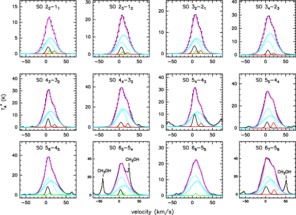
Figure 1: Gaussian fits to the observed SO lines. Dashed line for the plateau, cyan (solid line) for the high-velocity plateau, black for hot core, green for extended ridge, and red for the contribution of the component at 20.5 km s^-1. The total fit is shown in magenta. The data are the black histogram spectra.

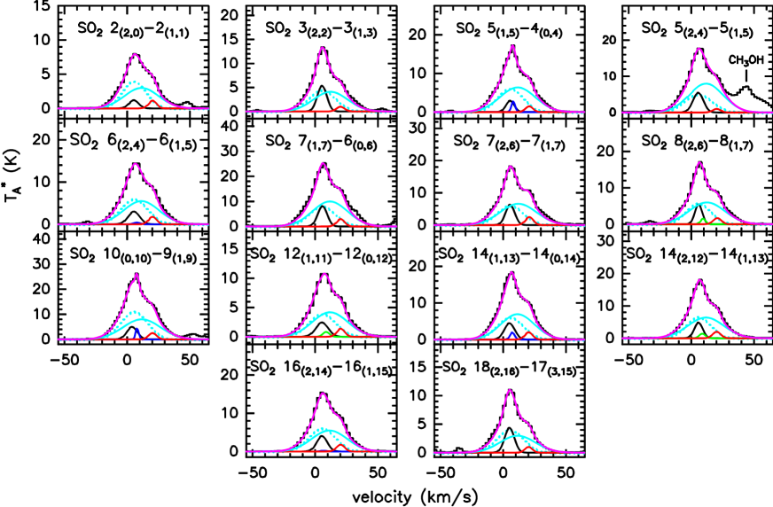
Figure 2: Gaussian fits for the SO₂ lines (2 mm data). The total fit is shown in magenta. Plateau is represented with the dashed line, high-velocity plateau in cyan (solid line), hot core in black, compact ridge in blue, extended ridge in green, and 20.5 km s^-1 component in red. The data are the black histogram spectra.

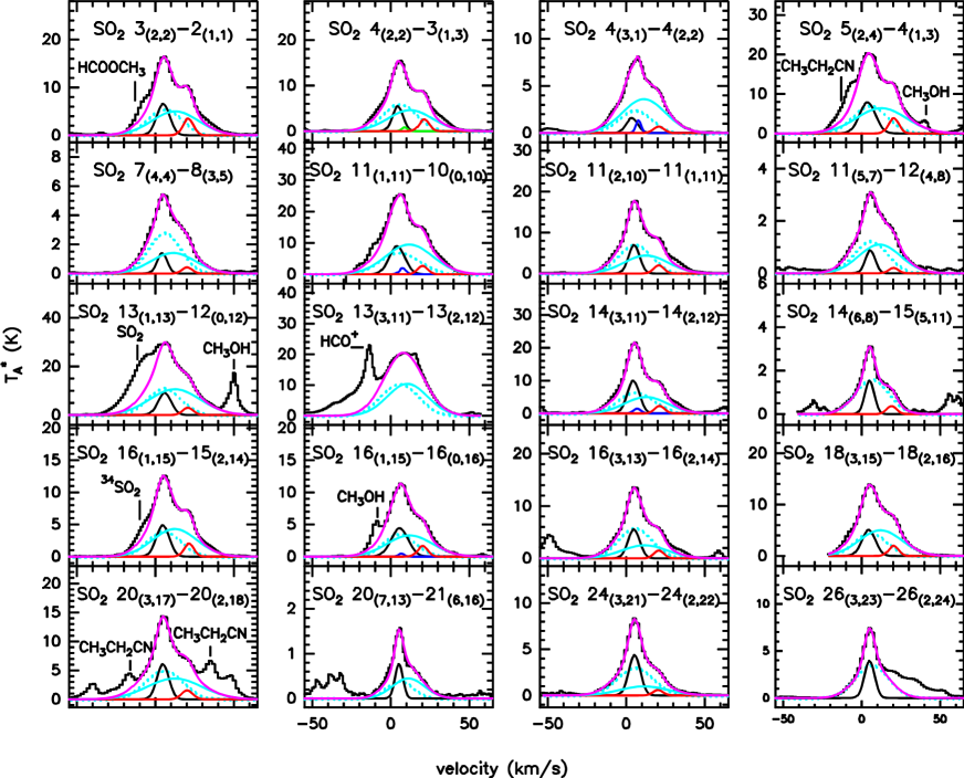
Figure 3: Gaussian fits for the SO₂ lines (1.3 mm data). The total fit is shown in magenta. Plateau is represented with the dashed line, high-velocity plateau in cyan (solid line), hot core in black, compact ridge in blue, extended ridge in green, and 20.5 km s^-1 component in red. The data are the black histogram spectra.

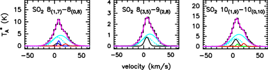
Figure 4: Gaussian fits for the SO₂ lines (3 mm data). The total fit is shown in magenta. Plateau is represented with the dashed line, high-velocity plateau in cyan (solid line), hot core in black, compact ridge in blue, extended ridge in green, and 20.5 km s^-1 component in red. The data are the black histogram spectra.

In total, the survey covers a bandwidth of 168 GHz, and of the 15,200 detected spectral features, about 10,700 have been identified and attributed to 45 molecules, including 191 isotopologues and vibrationally excited states (Tercero et al. 2010). We identify 20 lines of SO, 21 lines of ³⁴SO, 13 lines of ³³SO, and 14 lines of S¹⁸O. We also detect 166 lines of SO₂, 129 lines of ³⁴SO₂, 85 lines of ³³SO₂, 129 lines of SO¹⁸O, 74 lines of SO¹⁷O, and 78 lines of SO₂ v₂. Observed transitions of SO have a range of energy $E$_up between 16 and 100 K and a full width at half maximum (FWHM) of 40 km s^-1. In the case of SO₂ the energy range for the observed transitions is 12-1480 K and FWHM of 30-40 km s^-1 for transitions $J$$<$25 and FWHM $\sim$10-20 km s^-1 for transitions $J$$>$25. All these identifications are shown in Tables LABEL:table:tab_so and LABEL:table:tab_so2 (see Appendix). Those tables list the spectroscopic parameters of each transition, together with the observed line properties of the detected lines.

SO was the first molecule with a ³$\Sigma$ electronic ground-state detected in space by radio techniques (Gottlieb & Ball 1973). Its rotational levels are characterized by the rotational angular momentum quantum number, $N$, and the total angular momentum quantum number, $J$, which includes the contribution of the angular momentum of two unpaired electrons. For ³³S and ¹⁷O, the nuclear quadrupolar momentum couples with the rotation to produce a hyperfine splitting of the rotational levels. Selection rules for the electric dipole transitions are: $\Delta$$N$=$\pm$1, $\Delta$$F$=0, $\pm$1, and $\Delta$$J$=0, $\pm$1, in the absence of external fields. In the case of intermediate coupling, transitions are allowed for $\Delta$$N$=$\pm$ 3. The magnetic dipole transitions occur with the selection rules: $\Delta$$N$=0, $\pm$2 and $\Delta$$J$=0, $\pm$1. However, these transitions are extremely weak compared to the electric dipole transitions. We have estimated that the magnetic dipole allowed transitions SO will have intensities $\sim$1-6 mK, i.e., lines within the confusion limit of Orion ($T$${}^{\star}_{\mathrm{A}}$=20 mK).

SO₂ is an asymmetric molecule. The rotational energy levels are characterized by the three quantum numbers $J$, $K$_-1, and $K$₊₁. Since triatomic molecules are planar, the dipole moment components can only occur in the a- and b-axis directions. The selection rules for a-type transitions are $\Delta$$J$=0, $\pm 1$, $\Delta$$K$_-1=0, $\pm 2$, and $\Delta$$K$₊₁= $\pm 1$, $\pm 3$. For b-type transitions: $\Delta$$J$=0, $\pm 1$, $\Delta$$K$_-1= $\pm 1$, $\pm 3$, and $\Delta$$K$₊₁= $\mp 1$, $\mp 3$. SO₂ has its dipole moment along the b axis of the molecule. The nuclear quadrupolar momentum of ³³S and ¹⁷O also couples with the rotation leading to hyperfine structure.

As a starting point, we fitted each observed line with Gaussian profiles using CLASS to derive the contribution of each cloud spectral component (see Sect. 3.1). We assumed that the emission is optically thin and the observed lines are thermalized at a given temperature that was derived from rotational diagrams (see Goldsmith & Langer 1999), providing rotational temperatures for the different components of the cloud (Sect. 3.3). In Sect. 4 we use a radiative transfer code for a more advanced analysis of the LTE and non-LTE emission of SO and SO₂ species.

3.1 Line profiles

Figures 1, 2, 3, and 4 show the line profiles of some observed transitions of SO and SO₂, together with Gaussian fit results. To avoid degeneration, we fixed radial velocities ($v$_LSR) considering the characteristic values of each component of Orion KL. And we left the line width, the integrated intensity, and the antenna temperature as free parameters in the fits (in the results, we took the typical ranges of line widths into account for each component found in the bibliography, discarding those with large differences). In addition to the contribution from the usual components listed above, we also observe an unexpected emission peak centered on a velocity of $\simeq$20.5 km s^-1. We discuss its origin in Sects. 3.2 and 5.2.

We have detected 20 rotational transitions of SO, eight of which are blended with lines of other species. Figure 1 shows the contribution of the different cloud components to the emerging profile. We tried to fit the lines by considering only one plateau instead of two (at high and low velocity). First we centered this single plateau component on a velocity around 6-7 km s^-1, but with this we could not fit the part of the line profiles covering high ($>$20 km s^-1) velocities. With an increase in the line width of the fit, we reproduced this part of the profiles, but we overestimated the part of the lines that covers negative velocities. We found the opposite behavior if we fixed the single plateau component at higher velocities. Therefore we deduced that the best fits were obtained by considering two plateau components: one at low velocity, PL, ($\sim$6.5 km s^-1) and the other at high velocity, HVP, ($\sim$12 km s^-1). We observe that the emission mainly arises from these both plateau components. For transitions with angular momentum quantum number $N$$\lesssim$5, the strongest emission is found from the HVP, while for $N$$\gtrsim$5 PL presents the highest contribution to the emission. The contribution from the ER is very small. In this LTE analysis of SO, we have not considered the compact ridge component since its contribution is difficult to distinguish from the contribution from the HC. The parameters obtained from Gaussian fits for some of the SO lines are listed in Table 5 (see Appendix).

For SO₂ we have clearly identified 166 rotational transitions (see Figs. 2, 3, and 4). As indicated by their broad line profiles, we see that most of the emission comes from the plateau components, especially for transitions $J$$<$20 where the HVP plays an important role. However, for transitions $J$$>$20 the HC dominates. The parameters obtained for each component from Gaussian fits for SO₂ lines are listed in Tables 6 and 7 (see Appendix). Comparing this with SO lines, we see that the line profiles of both species are very similar.

3.2 The 20.5 km s^-1 feature and absorption at 15 km s^-1

Unlike the other species detected in the survey, we clearly observe an emission peak at $\simeq$20.5 km s^-1 in most SO and SO₂ lines. From Gaussian fits, we find that the line widths are $\sim$7.5 km s^-1. This feature presents an increase in the line intensity with frequency (i.e., with smaller beam). Figure 5 shows the integrated intensity, $W$, as a function of the frequency for the 20.5 km s^-1 component for SO lines. We see that, for the same line width, $W$ increases with frequency with a dependence as $\nu$². This means that the size of the region responsible for this velocity componenent is only a few arcseconds in diameter ($<$9$\arcsec$, smaller than the IRAM 30-m beam at the highest frequencies). The emission of this component could come from the interaction of the outflow with the ambient cloud; however, it should be noted that while in Orion-KL the $v$_LSR of the different components varies approximately between 3 and 10 km s^-1, Scoville et al. (1983) inferred that the $BN$ (Becklin-Neugebauer) object in Orion presents a significantly higher LSR velocity of around 21 km s^-1, therefore another possibility is that this feature located at 20.5 km s^-1 arises from the $BN$ source.

On the other hand, between the main emission peak of the line profiles of SO and SO₂ and this emission peak at 20.5 km s^-1, we observe a dip at $\simeq$15 km s^-1. Tercero et al. (2011) also find a velocity component at 15.5 km s^-1 in SiS emission lines ($\nu$=0), and one component of the SiO maser emission ($\nu$=1). Since the opacity is high for some lines of SO and SO₂, as well as for SiO, another possibility is that this dip may be the result of self-absorption. This could suggest that the SO and SO₂ dips at 15.5 km s^-1 are produced by the same gas observed in SiS. In Section 5 we draw firmer conclusions about the origin of the dip at 15.5 km s^-1 and of the peak at 20.5 km s^-1 from maps of SO and SO₂.

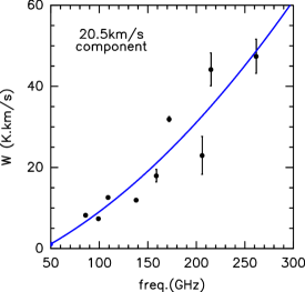
Figure 5: Integrated line intensities of the 20.5 km s^-1 component as a function of the line frequency for SO transitions.

3.3 Rotational diagrams

The results from the Gaussian fits have been used to build rotational diagrams for each species. This method involves the representation of the upper level column density normalized by the statistical weight of each rotational level versus the upper level energy, assuming optically thin emission filling the beam (see, e.g., Goldsmith & Langer et al 1999). The expression used to obtain the rotational diagrams, taking an optical depth ($C$_τ) different to unity into account, is

$$\mathrm{ln}({\gamma_{\mathrm{u}}W/g_{\mathrm{u}}})=\mathrm{ln}(N)-\mathrm{ln}(C_{\mathrm{\tau}})-\mathrm{ln}(Z)-(E_{\mathrm{u}}/kT),$$ (2)

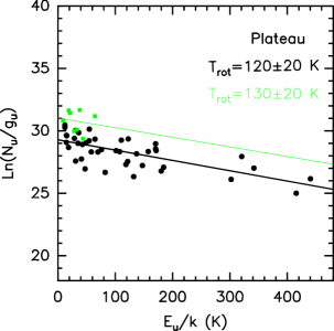
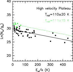
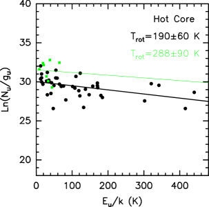
Figure 19: Rotational diagrams for the plateau, high-velocity plateau, and hot core components. Black dots for SO₂ and green dots for SO. The black and green lines are the best linear fits to the SO₂ and SO points, respectively.

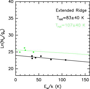
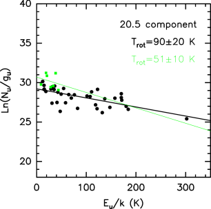
Figure 20: Rotational diagrams for the compact ridge, extended ridge, and 20.5 km s^-1 component. Black dots for SO₂ and green dots for SO. The black and green lines are the best linear fits to the SO₂ and SO points, respectively.

where $W$ is the integrated line intensity, $g$_u is the statistical weight of each level, $N$ the column density, $Z$ the partition function, $E$_u the level energy, $k$ the Boltzman constant, $T$ the temperature considering local thermodynamic equilibrium, and $\gamma$_u a constant that depends on the transition frequency and the Einstein coefficient $A$_ul (see Goldsmith & Langer 1999 for more details). Each cloud component is considered separately in the analysis. The rotational diagrams, shown in Figs. 19 and 20 (see Appendix), were obtained considering only lines without contamination from other species. The rotational temperatures obtained from SO₂ lines are plateau (PL)=120$\pm$20 K, hot core (HC)=190$\pm$60 K, high-velocity plateau (HVP)=110$\pm$20 K, compact ridge (CR)=80$\pm$30 K, extended ridge (ER)=83$\pm$40 and 20.5 km s^-1 component=90$\pm$20 K. The results from SO lines are (PL)=130$\pm$20 K, (HC)=288$\pm$90 K, (HVP)=111$\pm$15 K, (ER)=107$\pm$40 K, and 20.5 km s^-1 component=51$\pm$10 K. These results are shown in Table LABEL:table:rotational (see Appendix), together with the derived column densities and the optical depths. For each component, the obtained rotational temperatures for both molecules are consistent with each other, except for the HC where we obtain a large difference between both temperatures. This could indicate a temperature gradient in the hot core, or simply that the obtained rotational temperature could be overestimated due to the high scatter in the SO data. It would be necessary to have values of this species at higher energies in order to obtain firmer conlcusions. We observe that HVP presents a similar rotational temperature to the component of the plateau with lower velocity (PL). For the CR, we obtained a low temperature, probably due to the beam dilution, which is not corrected for in the rotational diagrams. From the diagrams, we also deduce that the new component at 20.5 km s^-1 is not a very warm region.

3.4 2′$\times$2′maps around IRc2

From the 2D line survey data of Orion KL, (Marcelino et al. in prep.), we produced integrated intensity maps of several SO and SO₂ transitions over different velocity ranges. Figure 7 shows the transitions 4_(2,2)-3_(1,3), 11_(1,11)-10_(0,10), and 14_(3,11)-14_(2,12) of SO₂; Fig. 6 shows the transitions 6₆-5₅ and 3₂-2₁ of SO; and Fig. 8 shows the transition 6₇-5₆ of ³⁴SO and the transition 28_(3,25)-28_(2,26) of ³⁴SO₂. Velocity intervals in the figures have been chosen to represent different source components. For all species and transitions, the strongest contribution arises from the velocity ranges 3-7 km s^-1 and 10-14 km s^-1, belonging to the HC and the HVP, respectively. The range 3-7 km s^-1 also includes PL velocities. These maps show elongated emission along the direction NE-SW. This agrees with Plambeck et al. (2009), who find (from SiO $J$=2-1 observations with an angular resolution of 0.45$\arcsec$) that the strongest emission arises from a bipolar outflow covering velocities from -13 to 16 km s^-1 along the NE-SW direction. This distribution is clearly seen in the maps of ³⁴SO and of SO (see lower panel in Fig. 6), especially in the ranges 7-10 km s^-1 (ridge) and 10-14 km s^-1 (HVP). Since the line widths corresponding to the HVP are the widest, with FWHM$\sim$ 30-40 km s^-1, altogether this suggests that the gas of the high velocity plateau is expanding in the direction NE-SW. On the other hand, the spatial distribution of ³⁴SO₂ is less extended and usually shows a peak to the NE of IRc2 (also seen in SO₂ and SO at velocities 3-7 km s^-1). For this species, the NE-SW distribution is better traced by the 20.5 component. This different behavior should be due to the high energy level ($E$_up=402.1 K) compared to the other mapped transitions, revealing the most compact and hottest regions in the KL cloud. Also evident on the maps is the new component at 20.5 km s^-1. From Figs. 7 and 6 we observe that its emission peak is located between the HC and BN positions.

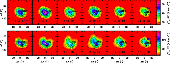
Figure 6: SO-integrated intensity maps over different velocity ranges (indicated at the bottom of each panel in km s^-1). Row 1 shows the transition 3₂-2₁ ($E$_up=21.1 K, $A$_ul=1.1x10^-5 s^-1, $S$=1.5). The interval between contours is 8 K km s^-1 and the minimum contour is 15 K km s^-1. Row 2 shows the transition 6₆-5₅ ($E$_up=56.5 K, $A$_ul=2.2x10^-4 s^-1, $S$=5.8). The interval between contours is 20 K km s^-1 and the minimum contour is 15 K km s^-1. The white cross indicates the position of the hot core and the black cross the position of the compact ridge.

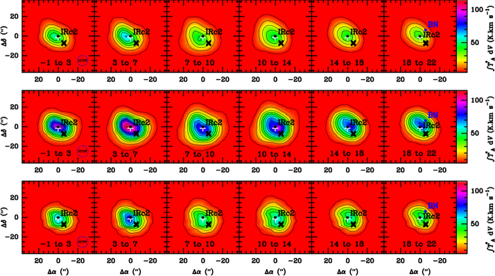
Figure 7: SO₂-integrated intensity maps over different velocity ranges (indicated at the bottom of each panel in km s^-1). Row 1 shows the transition 4_(2,2)-3_(1,3) (energy $E$_up=19 K, Einstein coefficient $A$_ul=7.7x10^-5 s^-1, and line strength $S$=1.7), row 2 the transition 11_(1,11)-10_(0,10) ($E$_up=60.4 K, $A$_ul=1.1x10^-4 s^-1, $S$=7.7), and the last row shows the transition 14_(3,11)-14_(2,12) ($E$_up=119 K, $A$_ul=1.1x10^-4 s^-1, $S$=8.1). The interval between contours is 10 K km s^-1, the minimum contour is 5 K km s^-1 and the maximum 155 K km s^-1. The white cross indicates the position of the hot core and the black cross the position of the compact ridge.

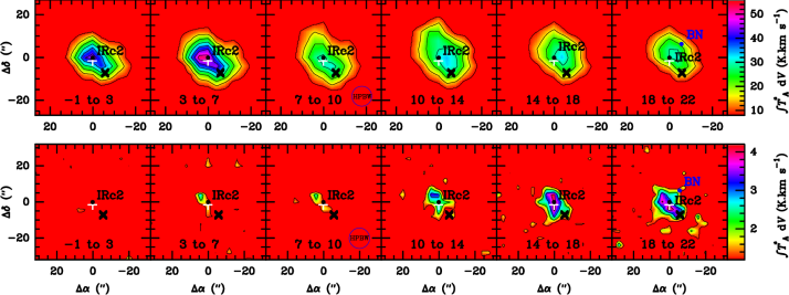
Figure 8: ³⁴SO and ³⁴SO₂-integrated intensity maps over different velocity ranges (indicated at the bottom of each panel in km s^-1). Row 1 shows the transition 6₇-5₆ of ³⁴SO ($E$_up=46.7 K, $A$_ul=2.2x10^-4 s^-1). The contour interval is 7 K km s^-1 and the minimum contour is 8 K km s^-1. Row 2 shows the transition 28_(3,25)-28_(2,26) of ³⁴SO₂ ($E$_up=402.1 K, $A$_ul=1.5x10^-4 s^-1). The interval between contours is 0.9 K km s^-1, and the minimum contour is 1.2 K km s^-1. The white cross indicates the position of the hot core and the black cross the position of the compact ridge.

4 Analysis

4.1 LVG models of the SO lines

In this section we analyze the non-LTE excitation and radiative transfer of SO lines. Following the study started by Tercero et al. (2010), we use an LVG (large velocity gradient) code, MADEX, developed by Cernicharo (2012) assuming that the width of the lines is due to the existence of large velocity gradients across the cloud, so that the radiative coupling between two relatively close points is negligible, and the excitation problem is local. The LVG models are based on the Goldreich & Kwan (1974) formalism. The final considered fit is the one that reproduces more line profiles better from transitions covering a wide energy range, within a $\sim$30$\%$ of the uncertainty in line intensity. For each component of the cloud, we assume uniform physical conditions (kinetic temperature, density, line width, radial velocity, and source size) that we choose taking into account the parameters obtained from the Gaussians fits of the line profiles, the rotational diagrams (with the derived rotational temperatures), and the mapped transitions.

Only for the HC do we consider LTE, which means that most transitions will be thermalized to the same temperature ($T$_rot$\simeq$$T$_K). If this condition was not satisfied, but we kept considering LTE approxmation, the temperatures would be overestimated, and this would produce a variation in the column densities. We cannot estimate whether they would be overestimated or underestimated since we do not know the population of each level. However, the HC of Orion presents a condition of temperature ($T$_K$>$200 K) and density ($n$(H₂)$\simeq$10⁷ cm^-3), which make the LTE assumption in this component feasible. Corrections for beam dilution are also applied for each line depending on the different beam sizes at different frequencies. Therefore, we fix all the above parameters (see Table LABEL:table:components_LVG) leaving only as a free parameter the column density fo each component. For the densitiy, $n$(H₂), we have adopted fixed values taken from typical values quoted in the literature. In order to determine the uncertainty of the values of hydrogen density and of temperature ($T$_K), we have run several models varying only the values for these parameters and fixing the rest.

Comparing the intensity differences between the spectra and the obtained line profiles for each case of $T$ and $n$, we deduce an uncertainty of 20 and 15$\%$ for the temperature and the hydrogen density, respectively. Although the parameter which could introduce higher uncertainty in the line profiles is the considered source size for each component, due to it varies depending on the molecular emission used for its determination. We fixed this parameter, as well as the hydrogen density, taking into account also the values used by Tercero et al. (2011) in her models of SiO and SiS. Other sources of uncertainty in the model predictions arise from the spatial overlap of the different cloud components. However, it has been possible to model their contribution thanks to the wide range of frequency and to the large number of lines from different isotopologues. We also find as a source of uncertainty the modest angular resolution of any single-dish line survey, pointing errors (errors as small as 2$\arcsec$ could introduce important changes in the contribution from each cloud component to the observed line profiles, especially at 1.3 mm), and line opacity effects. This last source of uncertainty becomes important when lines arising from the plateau are optically thick, causing an underestimation of the column densities of the components that are surrounded by the plateau (compact ridge, hot core, and the 20.5 km s^-1 component) along the line of sight (Schultz et al. 1999). In Tercero et al. (2010), these sources of uncertainty are explained in more detail. We estimate an uncertainty in our model intensity predictions of 25$\%$ for SO and ³⁴SO, and 35$\%$ for SO₂, ³⁴SO₂, ³³SO, S¹⁸O, ³³SO₂, and SO¹⁸O lines (higher uncertainty for SO₂ with respect to SO because of considering LTE instead of LVG approximation).

4.1.1 SO

Table 2: Physical parameters adopted for the Orion KL cloud components.

Component	Source diameter	Offset (IRc2)	$n$(H2)	$T$K	$\triangle$$v$FWHM	$v$LSR
	($\arcsec$)	($\arcsec$)	cm-3	(K)	(km s-1)	(km s-1)
Extended ridge (ER)	120	0	105	60	4	8.5
Compact ridge (CR)	15	7	106	110	3	8
High-velocity plateau (HVP)	30	4	106	100	30	11
Plateau (PL)	20	0	5$\times$106	150	25	6
Hot core (HC)	10	2	1.5$\times$107	220	10	5.5
20.5 km s-1 component	5	2	5$\times$106	90	7.5	20.5

To model the rotational lines of SO (listed in Table LABEL:table:tab_so, see Appendix), we used the collisional rates from Lique et al. (2006) for collisions with H₂. Figure 9 shows our best fit model. The component with the highest SO column density is the HVP, with $N$(SO)=(5$\pm$1)$\times$10¹⁶ cm^-2 (see Table LABEL:table:so_column_densities), although in the HC we also find a high column density with $N$(SO)=(9$\pm$3)$\times$10¹⁵ cm^-2. We find that the PL and the 20.5 km s^-1 component also contribute to the emission, but with a column density that is one order of magnitude lower than the HVP. We did not need to consider any contribution from the CR for SO. We could fit the narrow component by considering only the contribution from a single ridge (the extended ridge) at a temperature $T$_K=60 K. This agrees with the previous SO analysis in Sect. 3.1.

The model indicates that some SO lines with emission coming mainly from the high-velocity plateau are optically thick. The optical depths are $\tau$=1.1-1.4 for the transitions 6₅-5₄ and 6₆-5₅, and $\tau$=1.4-1.8 for the transitions 5₆-4₅ and 6₇-5₆. This means that the column densities obtained for the HC and 20.5 km s^-1 components, which are surrounded by the plateau, must be considered as lower limits, because the gas in the plateau components can absorb the emission from them. The HVP column density also has to be considered as a lower limit due to this opacity effect. We have also calculated the SO column density from the column density of ³⁴SO, whose lines are optically thin, and from the the solar abundance ratio ³²S/³⁴S=23 (Anders & Grevesse 1989). As we expected, Table LABEL:table:so_column_densities shows that the column densities of SO obtained from ³⁴SO are higher than those obtained from the fits. This confirms the presence of opacity effects on SO lines. We notice that the SO lines 2₁-1₂, 5₄-4₄, 6₅-, and 9₈-8₈ present a poor fit. This is because of the low Einstein coefficients $A$_ul and, mainly, to the low line strengths S ($<$4$\times$10^-6 s^-1 and $<$0.35, respectively) of these lines, which provides small fits. The profile lines that we observe for these transitions are probably caused by stronger emission from other species.

Compared with values obtained in previous studies, such as those of Turner et al. (1991) or Blake et al. (1987), who derived (from source-averaged) $N$(SO)$\sim$3$\times$10¹⁶cm^-2 in the plateau and N$\sim$3$\times$10¹⁵cm^-2 in the HC, we see our results agree. If we compare these results with our obtained column densities from ³⁴SO, we see that the plateau remains in agreement with these previous studies, but our column density in the HC is one order of magitude higher.

From the spatial distribution of the SO emission (Fig. 6), we find the integrated intensity peak to be in the velocity ranges 3-7 km s^-1 and 10-14 km s¹ for both transitions. These ranges correspond to emission arising mainly from the HC and the HVP, respectively, which agrees with the results obtained for the column densities in these regions. The transition with lowest energy (upper panel) shows a concentric emission distribution around IRc2, while for the transition with higher energy, the emission distribution is elongated toward NE-SW direction. We also observe that, for high energies, the emission peak in the velocity range 3-7 km s¹ is shifted toward the NE of the HC.

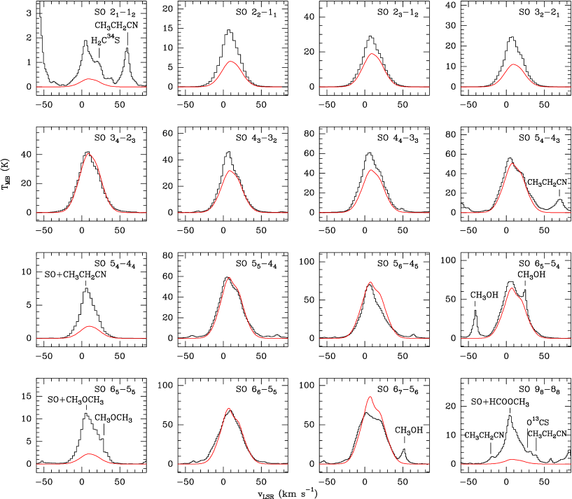
Figure 9: Observed lines of SO (black histogram) and best fit LVG model results (red).

4.1.2 ³⁴SO, ³³SO, and S¹⁸O

Figure 10 shows our best fit model for several rotational lines of ³⁴SO, which are listed in Table LABEL:table:tab_so (see Appendix). We find that the HVP is also responsible for most of the emission, together with the PL and the 20.5 km s^-1 component. According to our models, all transitions are optically thin with $\tau$$<$0.4, therefore this result is not considered to be a lower limit. The 20.5 km s^-1 component presents a similar column density to the HVP, and as for SO, its contributon is greater for higher $J$. In the HC we also find a strong contribution to the emission, however in the ER we find the lowest column density with $N$(³⁴SO)=(7$\pm$2)$\times$10¹² cm^-2.

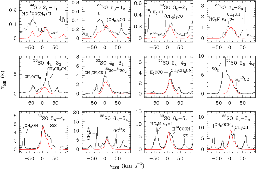
Figure 21: Observed lines of ³³SO (black histogram) and best fit LVG model results (red).

For the case of ³³SO we observe in Fig. 21 (see Appendix) that lines are partially blended with other species, which produces a large uncertainty in the derived fit. In addition, the hyperfine structure is noticeable in these transitions, adding more complexity to the line profiles. The fits for this isotopologue were done by adopting the calculated frequencies, intensities, and energies for hyperfine levels up to $N$=30 provided by the CDMS catalogs. We obtain similar column densities for all components, with $N$(³³SO)=(3-6)$\times$10¹⁴ cm^-2 (see Table LABEL:table:so_column_densities).

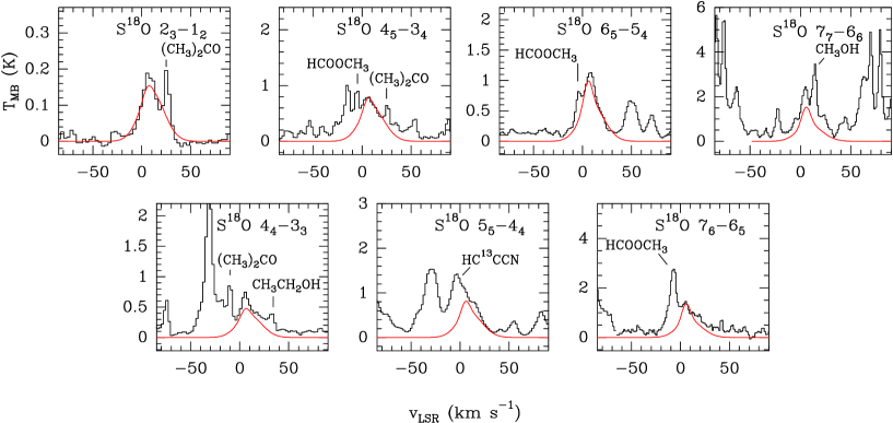
Figure 22: Observed lines of S¹⁸O (black histogram) and best fit LVG model results (red).

As was the case for ³³SO, some lines of S¹⁸O are blended with other species (Fig. 22 and Table LABEL:table:tab_so, see Appendix). In this case we also find similar column densities for all the components, $N$(S¹⁸O)=(1-5)$\times$10¹⁴ cm^-2, except for the CR, the ER, and the 20.5 km s^-1 component, where we do not find contribution to the emission.

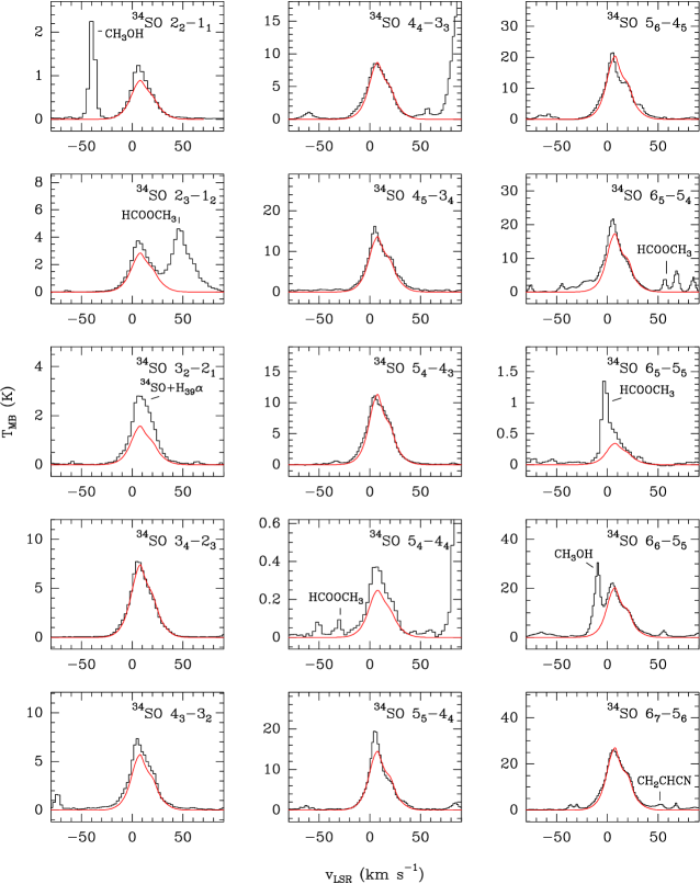
Figure 10: Observed lines of ³⁴SO (black histogram) and best fit LVG model results (red).

Table 3: Column densities, $N$, for SO and its isotopologues obtained from LVG model fits.

Component	SO	34SO	SO(a)	33SO	S18O
	$N$$\times$1015(cm-2)	$N$$\times$1015(cm-2)	$N$$\times$1015(cm-2)	$N$$\times$1015(cm-2)	$N$$\times$1015(cm-2)
Extended ridge (ER)	0.018$\pm$0.005	0.007$\pm$0.002	0.16$\pm$0.05	…	…
High-velocity plateau (HVP)	45$\pm$10	4$\pm$1	92$\pm$23	0.25$\pm$0.06	0.24$\pm$0.08
Plateau (PL)	5$\pm$1	3.0$\pm$0.8	69$\pm$19	0.5$\pm$0.2	0.10$\pm$0.04
Hot core (HC)	9$\pm$3	2.2$\pm$0.5	20$\pm$11	0.4$\pm$0.1	0.5$\pm$0.2
20.5 km s-1 component	5$\pm$1	3.5$\pm$0.8	81$\pm$19	0.6$\pm$0.2	…

4.1.3 S¹⁷O, ³⁶SO, and ³⁴S¹⁸O

Owing to the presence of other more intense species, we have detected neither S¹⁷O nor ³⁶SO in this survey, but from our data we derive upper limits for their column densities of $N$(S¹⁷O)$<$1.3$\times$10¹⁴cm^-2 and $N$(³⁶SO)$<$1.6$\times$10¹⁴cm^-2, respectively. We note that C³⁶S was detected by Mauersberger et al. (1996) in Orion. They found ³²S/³⁶S$\simeq$3500 which is consistent with our upper limit. We have not detected ³⁴S¹⁸O either; however, assuming the same physical conditions as those for the main isotopologue, we obtain an upper limit for its column density of $N$(³⁴S¹⁸O)$<$1.4$\times$10¹⁴cm^-2.

4.2 LTE models of the SO₂ lines

Due to the lack of collisional rates for levels with energies higher than 90 K, we have assumed LTE excitation to derive the SO₂ column densities. As stated before, this can overestimate or underestimate the calculated column densities. Given that we have collisional rates for SO, we ran our SO models again but considering LTE approximation, in order to compare the results. We observed that the new fits underestimated the line profiles, especially for low transitions. Probably this also happens with the SO₂ case, so we should consider our SO₂ column densities as lower limits. Table LABEL:table:tab_so2 (see Appendix) lists the 166 observed rotational lines. Figures 11, 12, 13, and 14 show a sample of 90 observed lines (ordered by increasing energy) with our best fits overlaid.

The main contribution to the emission of SO₂ comes from the HVP (affecting mainly the lines with energies $E$$<$400 K), with a column density of $N$(SO₂)=(1.3$\pm$0.5)$\times$10¹⁷cm^-2. The hottest region (the HC) also presents a similar high value, $N$(SO₂)=(1.0$\pm$0.4)$\times$10¹⁷cm^-2. We find that the CR presents a column density of $N$(SO₂)$\sim$10¹⁵cm^-2, whereas the 20.5 km s^-1 component presents the lowest contribution to the emission (Table LABEL:table:so2_column_densities).

If we compare our results for SO₂ with those of SO, we find that SO₂ column densities are about one order of magintude larger in all components, except in the 20.5 km s^-1 component, where SO presents a higher contribution to the emission. As for SO, we also calculated the SO₂ column densities from ³⁴SO₂ (optically thin lines) and the ³²S/³⁴S solar abundance ratio (Table LABEL:table:so2_column_densities). Except for the plateau components, we obtain that the column densities of SO₂ obtained from ³⁴SO₂ are larger than those obtained from fits, suggesting they are opacity effects on the SO₂ lines. Comparing with previous results, Blake et al. (1987) obtained (source-averaged) that SO₂ presents a column density in the plateau, $N$$\sim$10¹⁶cm^-2. Schilke et al. (2001) derived (beam-averaged) for the same region $N$(SO₂)=9.7$\times$10¹⁶cm^-2, which is very similar to our result in the high velocity plateau. For the HC, Sutton et al. (1995) found (also source-averaged) a column density, $N$(SO₂)$\sim$9$\times$10¹⁶cm^-2. Our results agree with these values; however, the large number of transitions that we observed let us determine more accurately that it is the lower temperature plateau component, i.e. the HVP, which contributes more to the emission of SO₂.

From the spatial distribution of the SO₂ emission (Fig. 7), we find the maximum integrated line intensity between the velocity ranges 3-7 km s^-1 and 10-14 km s^-1, as well as for SO. These velocity ranges correspond to emission of the HC and the HVP, respectively, which agrees with the column density results obtained above. The emission peak is located towards the NE of IRc2 for the range 3-7 km s^-1, while the emission peak for the HVP range is located $\sim$4$\arcsec$ to the SW of IRc2. Emission from the 20.5 km s^-1 component presents similar integrated intensity to the ridge (range of 7-10 km s^-1). On the other hand, the map of ³⁴SO₂ (Fig. 8) shows the strongest peak emission located northeast of IRc2 for all velocity ranges, although extended emission is seen to the southwest of IRc2, between 10 km s^-1 and 22 km s^-1. The ³⁴SO₂ transition shown in Fig. 8 has an upper energy level of $\sim$400 K and therefore may trace only the hottest component of the gas.

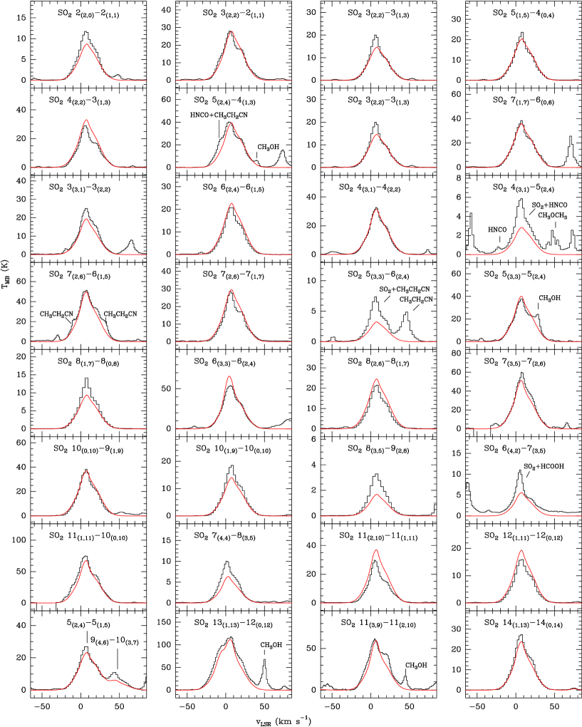
Figure 11: Observed lines (black histogram) of SO₂ with upper state energies lower than 400 K, ordered by increasing energy from top left to bottom right. Best fit LTE model results are overlaid in red.

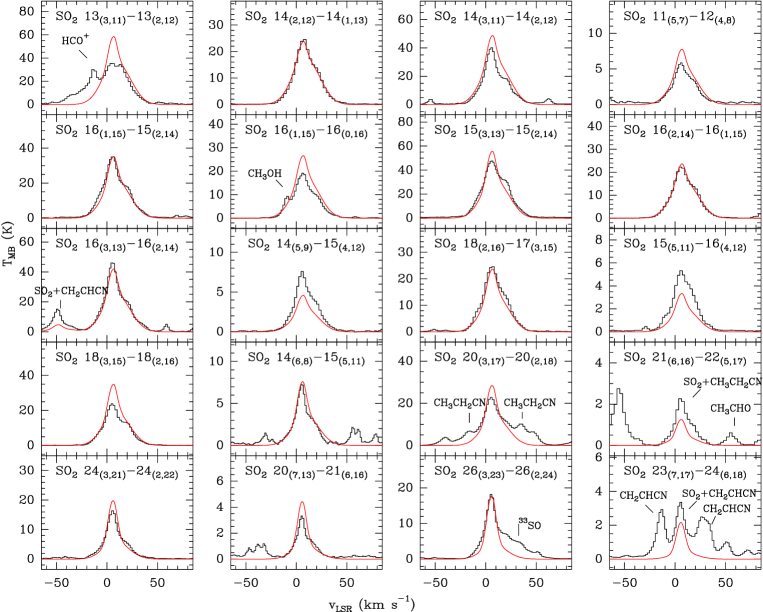
Figure 12: Observed lines of SO₂ (black histogram) with upper state energies lower than 400 K (continued), ordered by increasing energy from top left to bottom right. Best fit LTE model results are overlaid in red.

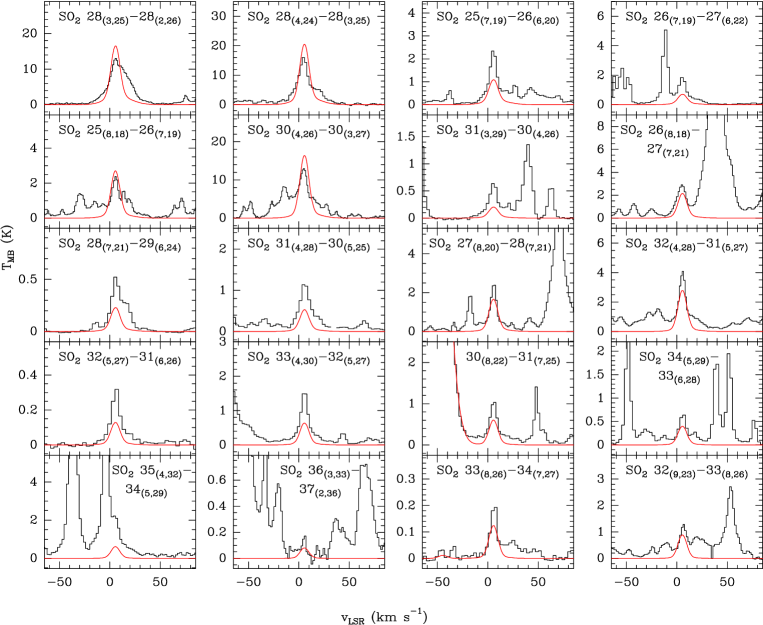
Figure 13: Observed lines of SO₂ (black histogram) with upper state energies between 400 K and 700 K, ordered by increasing energy from top left to bottom right. Best fit LTE model results are overlaid in red.

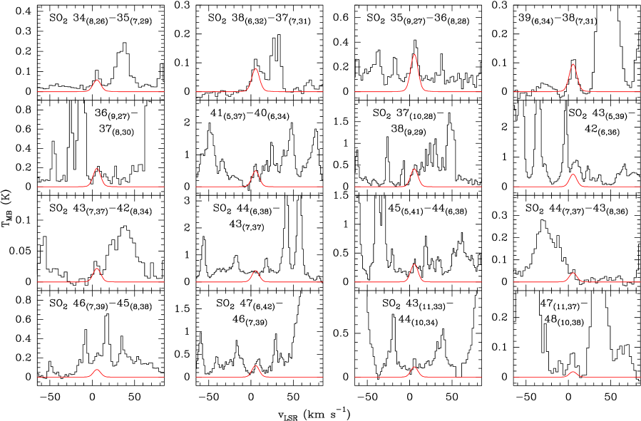
Figure 14: Observed lines of SO₂ (black histogram) with energies higher than 700 K, ordered by increasing energy from top left to bottom right. Best fit LTE model results are overlaid in red.

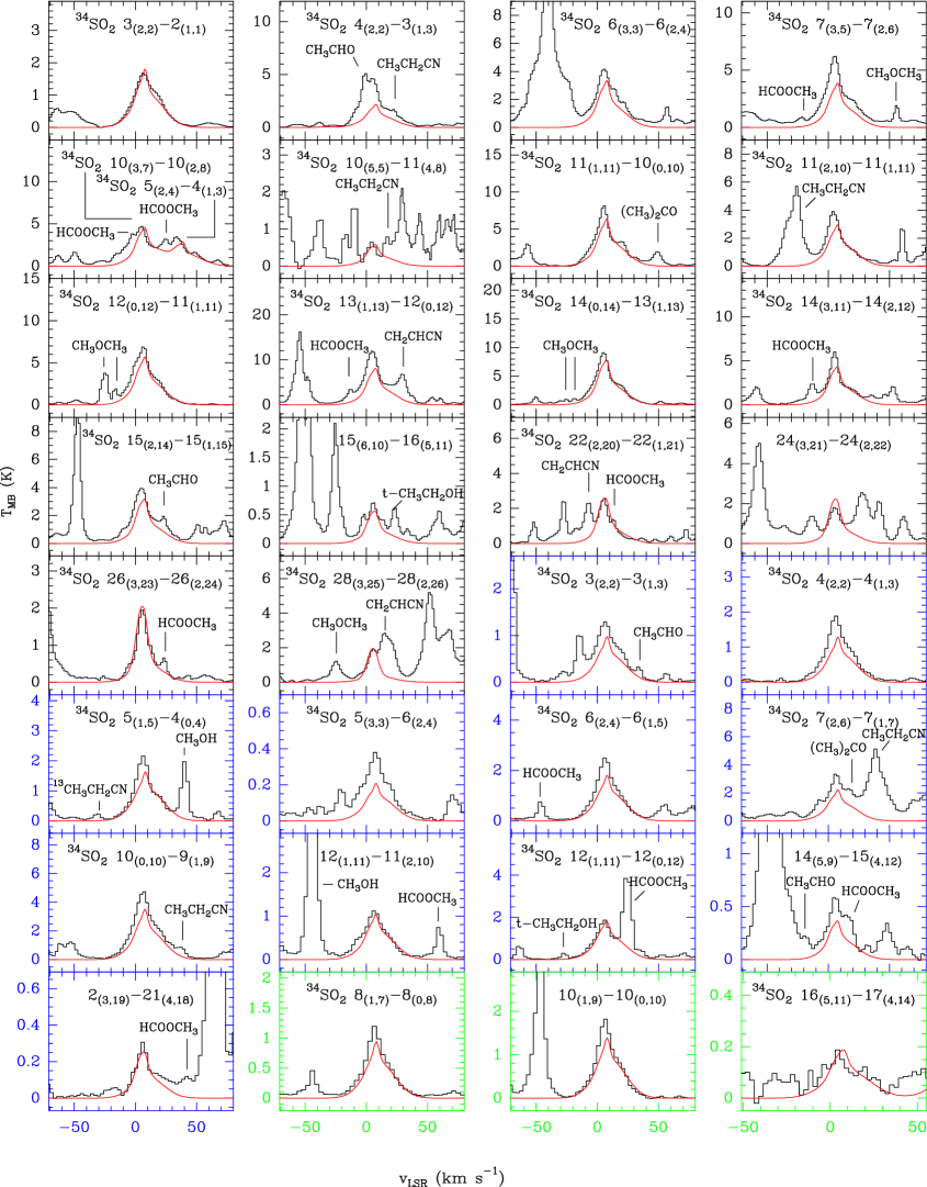
Figure 15: Observed lines of ³⁴SO₂ (black histogram). Best fit LTE model results are shown in red. Boxes with black, blue and green borders correspond to lines observed at 1.3, 2, and 3 mm, respectively.

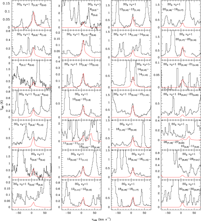
Figure 16: Observed lines of SO₂ $\nu$₂=1 (black histogram). Best fit LTE model results are shown in red.

4.2.1 ³⁴SO₂

We have detected 130 rotational lines of ³⁴SO₂ (Table LABEL:table:tab_so2 in Appendix). A sample of more than 30 lines is shown in Fig. 15.

This isotopologue, whose lines are optically thin, has the highest contribution to its emission from the HC, with $N$(³⁴SO₂)=(1.0$\pm$0.4)$\times$10¹⁶cm^-2. The other components with high column densities are the HVP and the PL with $N$(³⁴SO₂)=(7$\pm$2)$\times$10¹⁵cm^-2 and $N$(³⁴SO₂)=(6$\pm$2)$\times$10¹⁴cm^-2, respectively. Particulary interesting is the column density found in the ER, which presents the same order of magnitude as the PL. The same behavior is also observed in the isotopologues ³³SO₂ and SO¹⁸O, where the column densities in the ER are only 3 to 12 times lower than in PL. This could be due to the strong emission emerging from the HVP and HC affecting the excitation of the energy levels of this isotopologue in the ER, which means that line photons emitted from the inner components will be scattered by the lower density gas in the ER component (radiative scattering). For the compact ridge, we find the emission contributes mainly to the lines at low frequencies. The column density for ³⁴SO₂ obtained in the 20.5 km s^-1 component is about 100 times lower than for ³⁴SO (see Table LABEL:table:so2_column_densities).

4.2.2 ³³SO₂, SO¹⁸O, and SO¹⁷O

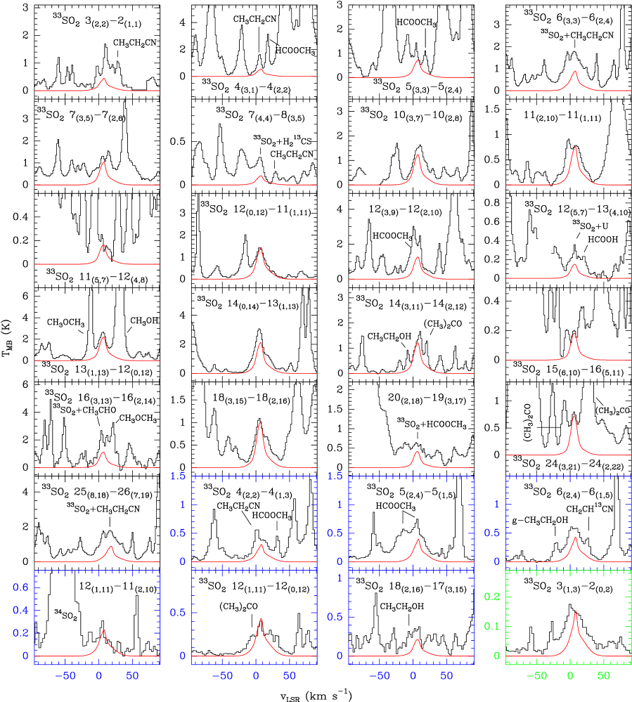
Figure 23: Observed lines of ³³SO₂ (black histogram) and best fit LTE model (red). Boxes in black, blue, and green correspond to frequencies at 1.3, 2, and 3 mm, respectively.

Figure 23 (see Appendix) shows transitions of ³³SO₂ in the frequency range covered at 1.3, 2, and 3 mm. Several of these are blended with other species, which makes the derived fits a bit biased. As for ³³SO, hyperfine structure affects the line profiles; however, we did not consider it in the ³³SO₂ model, so the derived column densities could be underestimated.

The most important contribution to the emission of ³³SO₂ comes from the hot core, with $N$(³³SO₂)=(4$\pm$1)$\times$10¹⁵ cm^-2, and from the HVP. The lowest contribution to the emission arises from the 20.5 km s^-1 component, with $N$(³³SO₂)=(9$\pm$3)$\times$10¹² cm^-2.

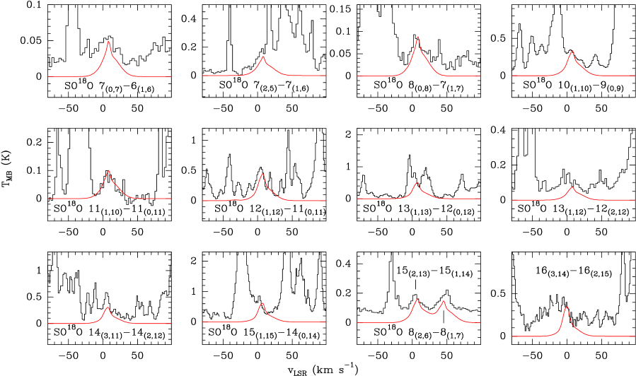
Figure 24: Observed lines of SO¹⁸O (black histogram) and best fit LTE model (red).

For SO¹⁸O (Fig. 24, see Appendix), the highest column density is also found in the HC, with $N$(SO¹⁸O)=(1.5$\pm$0.5)$\times$10¹⁵ cm^-2. The high-velocity plateau also presents an important contribution to the emission across the frequency range, whereas the PL mainly affects lines at 2 mm. The weakest contribution is from the ER, with $N$(SO¹⁸O)$\sim$10¹³ cm^-2.

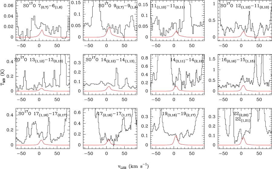
Figure 25: Observed lines of SO¹⁷O (black histogram) and best fit LTE model (red).

Figure 25 shows the spectra that contain some frequencies of SO¹⁷O, together with our best model. The maximum contribution to the emission of this isotopologue arises from the hot core with $N$(SO¹⁷O)=(8$\pm$3)$\times$10¹⁴ cm^-2. We find that the PL and HVP also contribute to the emission, but about four to eight times less than the HC. However, because all lines are weak ($T$_MB$<$0.3 K) and blended with other species, we should consider these results as upper limits.

4.2.3 SO₂ $\nu$₂=1

Figure 16 shows some of the detected lines of vibrationally excited SO₂ $\nu$₂, which are also listed in Table LABEL:table:tab_so2 (see Appendix). The hot core is responsible for most of the emission of this vibrational mode, with a column densitiy one order of magnitude higher than in the other components. From the column densities in the HC for SO₂ in its ground and vibrationally excited states, we can estimate a vibrational temperature, considering that

$$\frac{\exp(-E_{\mathrm{\nu_{x}}}/T_{\mathrm{vib}})}{f_{\mathrm{\nu}}}=\frac{N(SO_{2}\nu_{x})}{N(SO_{2})},$$ (3)

where $E$${}_{\mathrm{\nu_{x}}}$ is the energy of the vibrational state ($E$${}_{\nu_{2}}$=745.1 K), $T$_vib is the vibrational temperature, $N$(SO₂ $\nu$_x) is the column density of SO₂ in the excited vibrational state, $N$(SO₂) the total column density, and $f$_ν is the vibrational partition function, given by

$$f_{\mathrm{\nu}}=1+\exp(-E_{\mathrm{\nu_{3}}}/T_{\mathrm{vib}})+2\exp(-E_{\mathrm{\nu_{2}}}/T_{\mathrm{vib}})+\exp(-E_{\mathrm{\nu_{1}}}/T_{{\mathrm{vib}}}).$$ (4)

Taking into account that $N$(SO₂)=$N$_(ground)$\times$$f$_ν, we only need the energy of the vibrational state and the calculated column densities to derive the vibrational temperature.

We obtain $T$_vib=(230$\pm$40) K for SO₂ $\nu$₂=1. This value is similar to the kinetic temperature we assumed for the HC component (220 K). It is unlikely that the $\nu$₂=1 level at 745 K above the ground is excited by collisions. The main pumping mechanism could be IR radiation from the HC. A similar situation was found by Tercero et al. (2010) for OCS and other species.

4.2.4 ³⁴SO₂ $\nu$₂=1

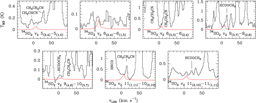
Figure 26: Observed lines of ³⁴SO₂ $\nu$₂=1 (black histogram) and best fit LTE model (red).

Figure 26 (see Appendix) shows some observed lines of ³⁴SO₂ $\nu$₂=1. The strongest emission comes from the hot core with $N$(³⁴SO₂ $\nu$₂=1)=(7$\pm$2)$\times$10¹⁴ cm^-2, although we also find a small contribution from the HVP and the CR, with $N$(³⁴SO₂ $\nu$₂=1)$\sim$5$\times$10¹³ cm^-2 for both. These contributions mainly affect the lines at 2 mm. Since all the lines we detect are very weak and mixed with other species, we should consider these results as upper limits.

Table 4: Column densities, $N$, for SO₂ and its isotopologues, obtained from LTE model analysis.

Component	SO2	34SO2	(a)SO2	33SO2	SO18O	SO17O	SO2 $\nu$2=1	34SO2 $\nu$2=1
	$N$$\times$1015	$N$$\times$1015	$N$$\times$1015	$N$$\times$1015	$N$$\times$1015	$N$$\times$1015	$N$$\times$1015	$N$$\times$1015
	(cm-2)	(cm-2)	(cm-2)	(cm-2)	(cm-2)	(cm-2)	(cm-2)	(cm-2)
Extended ridge	0.23$\pm$0.06	0.10$\pm$0.04	2.3$\pm$0.7	0.04$\pm$0.001	0.020$\pm$0.007	0.007$\pm$0.003	0.013$\pm$0.003	…
Compact ridge	1.2$\pm$0.4	0.5$\pm$0.2	12$\pm$2	0.07$\pm$0.02	0.03$\pm$0.01	0.007$\pm$0.003	0.20$\pm$0.05	0.05$\pm$0.02
High-velocity plateau	130$\pm$50	7$\pm$2	161$\pm$46	1.0$\pm$0.3	0.9$\pm$0.3	0.10$\pm$0.04	0.4$\pm$0.1	0.06$\pm$0.02
Plateau	10$\pm$3	0.6$\pm$0.2	14$\pm$3	0.5$\pm$0.2	0.06$\pm$0.02	0.03$\pm$0.01	…	…
Hot core	100$\pm$40	10$\pm$4	230$\pm$60	4$\pm$1	1.5$\pm$0.5	0.9$\pm$0.3	4$\pm$1	0.7$\pm$0.2
20.5 km s-1 comp.	0.17$\pm$0.06	0.04$\pm$0.01	0.8$\pm$0.2	0.009$\pm$0.003	…	…	…	…

4.3 Isotopic and molecular abundances

From the derived column densities of SO, SO₂, and their isotopologues, we can estimate abundance ratios. These are shown in Table 9 (see Appendix). We compare these ratios with solar isotopic abundance values from Anders & Grevesse (1989).

³²S/³⁴S: from the SO₂ lines we obtain a column density ratio for the PL of ³²S/³⁴S=16$\pm$10, in agreement with previous studies (³²S/³⁴S$\simeq$16 by Johansson et al. 1984, ³²S/³⁴S$\simeq$13-16 by Blake et al. 1987, and ³²S/³⁴S=15$\pm$5 by Tercero et al. 2010). For the HVP, ³²S/³⁴S=20$\pm$13, which is similar to the value for the solar isotopic abundance ratio and to the result deduced by Persson et al. (2007) where ³²S/³⁴S$\simeq$23$\pm$7. From the SO lines, with the exception of the HVP, we obtain low ratios for ³²S/³⁴S in comparison with the solar abundance, which could be due to opacity effects on the SO lines.

³²S/³³S: from $N$(SO)/$N$(³³SO) we obtain ³²S/³³S=180$\pm$80 for the HVP. This value agrees with the solar isotopic abundance ratio, 127, from Anders & Grevesse (1989). For the other three components, the obtained ratios are very low compared to the solar abundance, probably also due to the opacity effects for SO lines. These values should be considered as lower limits. We find similar behavior for the ratio $N$(SO₂)/$N$(³³SO₂).

³⁴S/³³S: from $N$(³⁴SO₂)/$N$(³³SO₂) we obtain ³⁴S/³³S=4$\pm$3 for the 20.5 km s^-1 component and ³⁴S/³³S=3-7 for the ridge (ER and CR), the HVP, and the HC. These values are similar to the solar abundance ratio (5.5). From $N$(³⁴SO)/$N$(³³SO) the obtained ratio is ³⁴S/³³S=6$\pm$3 for the HC and both plateau components.

¹⁶O/¹⁸O: our results for this ratio in the plateau agree with those obtained by Tercero et al. (2010), who derived ¹⁶O/¹⁸O=250$\pm$135 in the plateau from a study of OCS in this region. The compact ridge also presents similar ratio to that obtained by them. However, all these values are lower than the solar isotopic abundance ($\simeq$500).

SO/SO₂: in Fig. 18 we present the ratio $N$(SO)/$N$(SO₂) for the different components, as well as for the different isotopologues of SO and SO₂. We find that SO₂ is more abundant than SO in all components, except in the 20.5 km s^-1 component. In the HVP, SO₂ is three times more abundant than SO, while in the HC is up to 11 times more. However, in the 20.5 km s^-1 component, SO is $\sim$30 times more abundant than SO₂.

³⁴SO/³⁴SO₂: in the region affected by shocks, this ratio implies that ³⁴SO₂ is more abundant ($\sim$1.7 times) than ³⁴SO. In the hot core, we also find that ³⁴SO₂ is more abundant (5 times) than ³⁴SO, whereas in the ER the ratio is much larger (³⁴SO₂ is 14 times more abundant). As was found for SO/SO₂, the main difference is in the 20.5 km s^-1 component, where ³⁴SO is $\sim$100 times more abundant than ³⁴SO₂.

Table 10 shows the molecular abundances, $X$, of SO and SO₂ with respect to hydrogen in each component. They were derived using H₂ column density by means of the C¹⁸O column density, from the isotopic abundance ¹⁶O/¹⁸O, and assuming that CO is a good tracer of H₂ and therefore their abundance ratio is roughly constant. The column densities for H₂ are 7.5$\times$10²², 7.5$\times$10²², 2.1$\times$10²³, 6.2$\times$10²², 4.2$\times$10²³ cm^-2, and 1.0$\times$10²³ for the ER, CR, PL, HVP, HC, and the 20.5 km s_-1 component, respectively (see Tercero et al. 2011). We observe that the highest abundance of SO is obtained in the HVP, whereas in the HC and in the PL this abundance is $\sim$30 times lower. The extended ridge presents the lowest abundance of sulfur monoxide. The abundance of this molecule in the 20.5 km s_-1 component is about twice larger than in the HC. SO₂ is also more abundant in the HVP (between 8 and 600 times more abundant than in the rest of components). With respect to hydrogen, SO₂ is about one order of magnitude more abundant than SO in the HC and in the ER, while in both plateaus sulfur dioxide is only two-three times more abundant than SO.

4.4 Other sulfur-bearing molecules

We provide here upper limits for the column densities of several sulfur-bearing molecules not detected in our survey. We have assumed the same spectral components as for SO and SO₂ (HC, PL, HVP, CR, and ER) and an LTE approximation, due to the lack of available collision rates. Table LABEL:table:components_LVG shows the adopted temperature values, among other parameters, for each component, and Table LABEL:table:upper_limits (see Appendix) shows the results obtained, the dipole moment of each species, and references for the spectroscopic constants. The upper limit of column density for each species were obtained summing the contribution of all the components.

SO⁺: first detected in the interstellar medium towards the supernova remnant IC443 (Turner et al. 1992), it was proposed as a tracer of dissociative shocks, although later surveys carried out in dark clouds, star-forming regions, and high velocity molecular outflows suggest that this reactive ion is not associated with shock chemistry (Turner et al. 1994). SO⁺ presents a high abundance in PDRs like NGC 7023 and in the Orion Bar (Fuente et al. 2003). In Orion KL, we obtain an upper limit to its column density of $N$(SO⁺)$\leq$2.5$\times$10¹⁴ cm^-2, providing an abundance ratio of $N$(SO)/$N$(SO⁺)$\geq$2080. This result implies that UV radiation does not play an important role in this region.

($cis$)-HOSO⁺: it is the most stable isomeric form of this ion. This species has not yet been detected in the interstellar medium, but its large dipole moment (1.74 D), its easy formation through H${}^{+}_{3}$ reacting with SO₂ and the fact that it does not react with H₂ make this ion an excellent candidate for being detected, mainly in hot regions where the parent SO₂ is very abundant. The upper limit calculated for this ion is $N$($cis$-HOSO⁺)$\leq$3.6$\times$10¹³ cm^-2.

SSO: this molecule has not been detected yet in the interstellar medium, but it is a plausible candidate, since the oxides SO and SO₂ are particulary abundant, especially in star-forming regions. Disulfur monoxide (SSO) was spectroscopically studied first by Meschi & Myers (1959) who detected rotational transitions in the ground vibrational state and in the $\nu$₂=1 state. Later, Thorwirth et al. (2006) carried out a millimeter and submillimeter wave investigation of SSO in the ground vibrational state to frequencies as high as 470 GHz. We have not detected SSO in our line survey, but we obtain an upper limit for its column density of $N$(SSO)$\leq$7.6$\times$10¹⁴ cm^-2, providing an abundance ratio of $N$(SO)/$N$(SSO)$\geq$1155.

OSiS: silicon oxysulfide was first characterized in the gas phase at high spectral resolution by Thorwirth et al. (2011). It prosseses a large dipole moment ($\mu$_a=1.47 D) and its bond distances are very short in comparison with those of SiO and SiS. It has not been detected yet in the interstellar medium, and we obtained an upper limit for the column density of this molecule in Orion KL of $N$(OSiS)$\leq$6.3$\times$10¹³ cm^-2. Tercero et al. (2010) found that in Orion KL the total column density for SiS in the ground state is $N$(SiS)=(1.4$\pm$0.4)$\times$10¹⁵ cm^-2. This result provides an abundance ratio of $N$(SiS)/$N$(OSiS)$\geq$22.

S₃: thiozone is a bent chain with a bond to the apex S whose rotational spectrum was first measured by McCarthy et al. (2004). S₃ has not yet been observed in the interstellar medium; however, it is an excellent candidate for astronomical detection in rich interstellar sources. In addition, S₃ may also exist in the atmosphere of Io, where S₂ has already been detected in the ultraviolet. Owing to the presence of more intense lines from other species we have not detected S₃ in our line survey. We provide an upper limit for its column density of $N$(S₃)$\leq$1$\times$10¹⁵ cm^-2.

S₄: tetrasulfur is a singlet planar trapezoid whose rotational spectrum was observed for the first time by McCarthy et al. (2004). S₄ has a substantial dipole moment, 0.87 D, hence an intense rotational spectrum across the entire radio band. The upper limit column density we calculated for this molecule is $N$(S₄)$\leq$7$\times$10¹⁴ cm^-2.

CH₃SOCH₃: Barnes et al. (1994) obtained this molecule in the laboratory while investigating the gas-phase reaction of OH with the oxidation of dimethyl sulfide at room temperature. Dimethyl sulfoxide has not been observed yet in the interstellar medium, but we provide an upper limit for its column density of $N$(CH₃SOCH₃)$\leq$1$\times$10¹⁴ cm^-2.

H₂CSO: sulfine was first identified in 1976 as a product of the pyrolysis of a variety of sulfur-bearing precursors. H₂CSO is a planar molecule of C_s symmetry. Joo et al. (1995) analyzed its infrared spectrum at high resolution. We provide an upper limit for the column density for this undetected molecule in the interstellar medium of $N$(H₂CSO)$\leq$3$\times$10¹³ cm^-2.

HNSO: thionylimide is a semi-stable molecule that adopts a cis-planar structure of C_s symmetry in the ground state. HNSO is the simplest molecule in the group of organic nitrogen-sulfur compounds. We calculated an upper limit for its column density of $N$(HNSO)$\leq$4.1$\times$10¹⁴ cm^-2, which provides an abundance ratio $N$(SO)/$N$(HNSO)$\geq$2600.

o-H₂S₂: the rotational spectrum of disulfane (H₂S₂) has been measured in the far-infrared, millimeter, and submillimeter (Winnewisser et al. 1966). The density of its spectrum is enhanced by the presence of low-lying torsional and S-S stretching modes. We did not observe this molecule in our line survey but we provide an upper limit for its column density of $N$(o-H₂S₂)$\leq$1.6$\times$10¹⁴ cm^-2.

SSH and H₂SO₄: these molecules have not yet been detected in the interstellar medium. The calculated upper limits for their column densities are $N$(SSH)$\leq$7.1$\times$10¹³ cm^-2 and $N$(H₂SO₄)$\leq$1.3$\times$10¹⁴ cm^-2, respectively.

CH₃SSH: methyl hydrodisulfide has not been observed in the interstellar medium. Tyblewski et al. (1986) studied its rotational spectrum, together with that of CH₃SSD, between 18 and 40 GHz providing rotational constants. We derive an upper limit for its column density of $N$(CH₃SSH)$\leq$2.6$\times$10¹⁴ cm^-2.

($tr$)-HCSSH: the spectrum of dithioformic acid has been studied by Bak et al. (1978), who assigned the rotational transitions of this species in its ground state to a $trans$ and $cis$ rotamer. We provide an upper limit for the column densitiy of ($tr$)-HCSSH (more stable) $N$$\leq$3.6$\times$10¹³ cm^-2.

5 Discussion

There have been many spectral line surveys of Orion KL aimed at determining the physical and chemical structure of this region (e.g., Blake et al. 1987, Sutton et al. 1995, Schilke et al. 2001). The survey analyzed here was first presented by Tercero et al. (2010), covers the widest frequency range of all of them (80-281 GHz). Due to this wide range and to the large number of observed transitions of SO, and particularly of SO₂, it has been possible not only to determine the structure of the cloud (gas temperature, gas density, size of components, etc.) with better accuracy (the 3 mm window shows best the coldest regions, such as the ER, whereas the 1.3 mm window probes the warmest regions), but also to demonstrate the need for considering a density and temperature gradient in the HC of Orion KL. From rotational diagrams, we found a large difference ($\sim$100 K) between the rotational temperatures of SO and SO₂, indicating the possibility of a hotter inner region to the HC. We draw the same conclusion from the fits for SO₂ lines with energies $E$$>$400 K. To obtain better fits for lines with energies $E$$>$700 K, we considered a high column density for the HC, which overestimates in the fit for the lines with energy around 400 K (see Figs. 12 and 13). But by considering an additional inner component to the HC with higher temperature, it would probably be possible to obtain a better fit to the lines with high energies, while avoiding overestimation of lines with intermediate energies. To test this possibility, we fit the SO₂ line profiles with energies $E$$>$700 K considering a hotter ($T$_K=280 K) HC (affecting only the highest energy transitions), with $n$(H₂)=5$\times$10⁶ cm^-3, located at 5.5 km s^-1, and with $\triangle$$v$_FWHM=7 km s^-1. For a SO₂ column density of (4$\pm$1)$\times$10m¹⁶ cm^-2, we improve the line profile fits of these high energies transitions (see Fig. 17). This shows the existence of a temperature and density gradient in the HC of Orion KL. However, its structure should be determined accurately with observations of SO and SO₂ (and mainly of its isotopologues, which are optically thin) at higher frequencies with telescopes such as APEX.

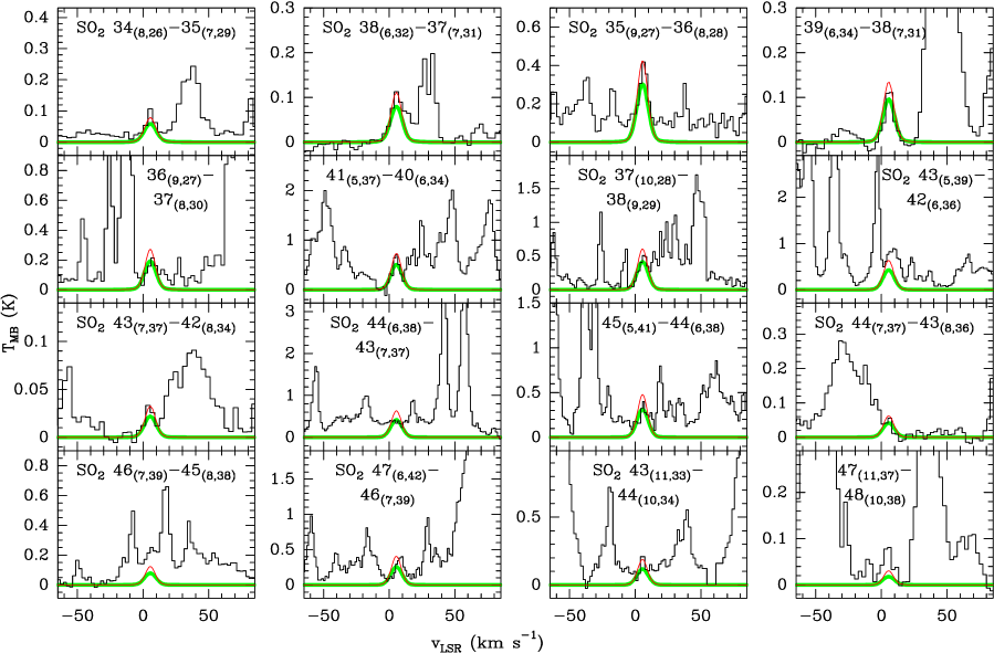
Figure 17: Observed lines of SO₂ (black histogram) with energies higher than 700 K, ordered by increasing energy from top left to bottom right. Best fit LTE model results considering a hot core at $T$_K=220 K (green curve) and with a hot core at $T$_K=280 K (red curve).

On the other hand, the large number of observed lines of the ³⁴S and ³³S isotopologues has allowed us to calculate column densities and isotopic and molecular abundances that are key to understanding the chemical evolution of this region.

5.1 SO and SO₂ as tracers of shocks and hot gas

In Section 4 we showed that an important contribution to the emission of SO and SO₂ comes from the HC component of Orion KL. In Fig. 18 we plotted the ratio of $N$(SO)/$N$(SO₂) for the different components, as well as for the different isotopologues of SO and SO₂. The figure shows that the column density of SO₂ in the HC is higher than that for SO. We should take into account that our column densities for SO₂ may have been slightly underestimated because of using an LTE model to infer the column density (instead of LVG, as was used for SO). For that reason, we considered a higher uncertainty (35$\%$) in the model intensity predictions for SO₂, than for SO (20$\%$), as said previously. Moreover, the opacity may affect SO and SO₂ differently, which would in turn affect their column density ratio. But if we consider the result of the ratio ³⁴SO/³⁴SO₂ in the hot core, we observe that SO₂ continues to be more abundant than SO. This could indicate that SO₂ is a better tracer of warm gas than SO.

Our results are consistent with predictions from chemical models of hot cores (e.g., Hatchell et al. 1998). Viti et al. (2004a) modeled the evaporation of ices near massive stars and found that SO₂ becomes more abundant than SO in the hot core from 31.500 years after the formation of a high-mass star. For shorter timescales, SO is much more abundant than SO₂. Thus, the SO/SO₂ ratio could be regarded as a chemical clock (which should decrease with time), and our results showing a lower SO/SO₂ ratio for the HC component seem to suggest a late stage for the hot core evolution in Orion KL.

On the other hand, the ratio of SO/SO2 is higher in the PL and the HVP than in the HC and the ER (see Fig. 18), and in particular for the PL, this ratio reaches values close to or even higher than 1. Since SO is a well-known outflow tracer (e.g., Chernin et al. 1994; Codella & Scappini 2003; Lee et al. 2010; Tafalla et al. 2010), and SO seems to be more enhanced than SO2 in shocks (from an observational point of view, e.g., Codella & Bachiller (1999), Jiménez-Serra et al. (2005), and from a theoretical point of view, e.g., Viti et al. (2004b); Benedettini et al. (2006), for timescales $\sim$10,000 yr), it seems very feasible that the high SO/SO₂ ratios measured in the (high velocity) plateau are the consequence of a definite enhancement of the SO abundance with respect to SO₂, due to shocks propagating into the surrounding medium of Orion KL.

5.2 Nature of the 15 km s^-1 dip and 20.5 km s^-1 velocity component

To properly fit the SO and SO₂ spectra in Orion KL, a new velocity component at 20.5 km s^-1 had to be included in the model (see Section 3.2). In addition, a possible dip at 15.5 km s^-1 in the SO and SO₂ spectra has been identified. The dip at 15.5 km s^-1 could be self-absorption due to the high opacity of the observed transitions. However, in all cases, the line strength $S$ is uncorrelated with the amount of absorption. For example, the transition 11_(1,11)-10_(0,10) of SO₂, with a line strength of $S$=7.7 and Einstein coefficient $A$_ul=1.1x10^-4 s^-1, would be expected to display more self-absorption and therefore a lower integrated intensity than the transition 4_(2,2)-3_(1,3) with $S$=1.7 and $A$_ul=7.7x10^-5 s^-1, but we see the opposite (especially in the range at 14.5-16.5 km s^-1). In addition, we obtain in Fig. 7 a high integrated intensity in the velocity range 14-18 km s^-1, when the integrated intensity in the ranges 10-14 km s^-1 and 18-22 km s^-1 is also large. Altogether, this suggests that the emission at 15 km s^-1 is only the sum of contributions of emission coming from the HVP and the 20.5 km s^-1 component.

With respect to the nature of the emission at 20.5 km s^-1, Fig. 18 shows that the column density ratio of SO/SO₂ of this component is about two to three orders of magnitude higher than the other velocity components in Orion KL. This is also true for the ³⁴SO/³⁴SO₂ and ³³SO/³³SO₂ ratios, suggesting that it is not an opacity effect. Such a high ratio could be due in part to filling factor problems, if the 20.5 km s^-1 component is much more compact in SO₂ than in SO, and/or could be the result of applying a different method (LVG for SO vs LTE for SO₂) to infer the column densities. However, the large difference compared to the other components suggests that it is a definite chemical effect, and since the SO/SO₂ ratio is higher in regions associated with shocks such as the HVP and the PL (Sect. 5.1), the 20.5 km s^-1 component could be related to shocks as well, maybe associated with the explosive dynamical interaction that took place in Orion KL (Gómez et al. 2005, Zapata et al. 2011a) and more especifically to shocks associated with the BN object. This is consistent with the fact that the BN object in Orion presents significantly high CO and ¹³CO emission at $\sim$20 km s^-1 (Scoville et al. 1983). Observations combining both single-dish and interferometric data are required to definitely identify the spatial region in Orion KL emitting the bulk of emission at 20 km s^-1 .

6 Summary and Conclusions

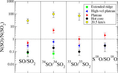
Figure 18: Ratio $N$(SO)/$N$(SO₂) for each component and for the different isotopologues of SO and SO₂.

This study is part of a series of papers with the goal of analyzing the physical and chemical conditions of Orion KL. The study is divided into different molecular families, and here we have focused on the emission lines of SO and SO₂ and their isotopologues. We have analyzed the IRAM 30-m line survey of Orion KL observed by Tercero et al. (2010), which covers the frequency range 80-281 GHz. We identified more than 700 rotational transitions of these molecules, including lines from the vibrational state $\nu$₂=1 of SO₂ and the isotopologue SO¹⁷O, detected for the first time in the interstellar medium. This large sample has let us improve our knowledge about the physical and chemical conditions in Orion KL, especially due to the observation of a large number of SO₂ transitions at high energies. The analysis of SO and SO₂ was carried out using an LTE and LVG radiative transfer model, taking the physical structure of the source into account (hot core, compact ridge, extended ridge, and plateau components).

First, we fit SO and SO₂ lines with Gaussian profiles to obtain an approximate $T$_rot value in each component. We detected a dip at $\sim$15 km s^-1 in most of the lines and an emission peak centered on 20.5 km s^-1. For the dip at 15 km s^-1, we discarded self-absorption as a possible cause, concluding instead that the weak emission is due to the sum of small contributions coming from the high velocity plateau and from the 20.5 km s^-1 feature, which corresponds to an unresolved component ($\sim$5$\arcsec$´´ diameter), with line width of $\sim$7.5 km s^-1 and with an especially high column density of SO in comparison to SO₂. Its rotational temperature is 50$\pm$10 K from SO lines and 90$\pm$20 K from SO₂ lines. For the rest of the components, the rotational temperatures obtained from SO₂ lines are: plateau (PL)=120$\pm$20 K, hot core (HC)=190$\pm$60 K, high velocity plateau (HVP)=110$\pm$20 K, compact ridge (CR)=80$\pm$30 K, and extended ridge (ER)=83$\pm$40. The results from SO lines are: (PL)=130$\pm$20 K, (HC)=288$\pm$90 K, (HVP)=111$\pm$15 K, and (ER)=107$\pm$40 K.

The second part of the analysis was carried out using a radiative transfer code. For the case of SO, we analyzed its non-LTE excitation, however, for SO₂ we assumed LTE excitation due to the lack of collisional rates for energies higher than 90 K (we observe SO₂ lines with energies up to 1500 K). We found that most of the emission of SO₂ and SO arises from the high-velocity plateau, with column densities of $N$(SO₂)=(1.3$\pm$0.3)$\times$10¹⁷ cm^-2 and $N$(SO)=(5$\pm$1)$\times$10¹⁶ cm^-2, respectively, and from the hot core, in particular in the case of SO₂, whose column density is similar to that obtained in the high-velocity plateau. These values are up to three orders of magnitude higher than the column densities obtained for the ridge components. These results let us conclude that SO and SO₂ are not good tracers only of shock-affected areas, but also of hot dense gas. In addition, from the ratios ³⁴SO/³⁴SO₂, ³³SO/³³SO₂, and S¹⁸O/SO¹⁸O₂ in the different components of the cloud, we observe that in the high-velocity plateau (region affected by shocks) sulfur dioxide is up to five times more abundant than SO. The same trend is found in the hot core.

We have also carried out 2$\arcmin$$\times$2$\arcmin$ mapping around Orion IRc2 in a number of lines of SO, SO₂, and their ³⁴S isotopologues. In Sect. 3.4 we presented maps of three transitions of SO₂ (Fig. 7), two transitions of SO (Fig. 6), one transition of ³⁴SO and one of ³⁴SO₂ (Fig. 8). We plotted different velocity ranges for each transition to explore the spatial distribution of the emission. In agreement with our column density results, we found the maximum integrated intensities in the range containing the hot core (3-7 km s^-1) and in the range 10-14 km s^-1 (corresponding to the high velocity plateau), whose emission peak is centered approximately 4$\arcsec$ to the southwest of IRc2. In all mapped transitions, but especially in those of SO and ³⁴SO, we observe an elongation of the gas along the NE-SW direction. In these maps, we also detected a strong emission in the velocity range located at 20.5 km s^-1. From the spatial distribution of this feature and from the analysis of the line profiles, we suggest that this emission is probably related to shocks associated to the $BN$ source or to a gas cloudlet ejected in the explosive event that could have taken place in Orion KL.

In this paper, we have also demonstrated the need to consider a temperature and density gradient in the hot core of Orion KL, with a comparison between fits of SO₂ line profiles at high energies, assuming two different temperatures ($T$_K=220 K and $T$_K=280 K) in the hot core. Only with the low temperature it was not possible to obtain good line fits for $E$$>$700 K, without avoiding overestimation for lines with intermediate energies. In addition, the large difference between the rotational temperatures in the hot core and the need to consider a large contribution to the SO₂ isotopologue emission in the extended ridge support the conclusion of the presence of temperature and density gradients in Orion KL. However, it would be necessary to also consider emission lines (mainly from isotopologues) spanning a wider frequency range with observations from other telescopes, such as APEX, in order to determine these gradients accurately. Moreover, to describe this molecular cloud in greater detail while avoiding spectral confusion would require interferometric observations with higher spectral resolution and higher sensitivity (such as those provided by ALMA).

Appendix A Figures and tables

Table 5: SO emission line parameters obtained from Gaussian fits.

Species/	Plateau			High-velocity plateau			Hot core			Extended ridge			20.5 km s-1 component
Transition	$v$LSR	$\Delta$$v$	$T$${}^{\star}_{\mathrm{A}}$	$v$LSR	$\Delta$$v$	$T$${}^{\star}_{\mathrm{A}}$	$v$LSR	$\Delta$$v$	$T$${}^{\star}_{\mathrm{A}}$	$v$LSR	$\Delta$$v$	$T$${}^{\star}_{\mathrm{A}}$	$v$LSR	$\Delta$$v$	$T$${}^{\star}_{\mathrm{A}}$
	(km s-1)	(km s-1)	(K)	(km s-1)	(km s-1)	(K)	(km s-1)	(km s-1)	(K)	(km s-1)	(km s-1)	(K)	(km s-1)	(km s-1)	(K)
SO 22-11	6.8	27$\pm$3	3.86	10.8	34$\pm$1	5.00	5.5	11.2$\pm$0.3	2.20	8.8	6.5$\pm$0.4	1.10	20.5	8.5$\pm$0.5	0.91
SO 23-12	6.6	27$\pm$1	6.70	11.7	35$\pm$1	11.0	5.5	10.5$\pm$0.5	4.20	8.5	5.6$\pm$0.2	1.51	21.0	7.5$\pm$0.4	0.93
SO 32-21	6.8	27$\pm$5	7.00	11.8	34$\pm$2	7.15	5.3	11.5$\pm$0.8	3.70	9.0	5.4$\pm$0.2	1.50	20.5	7.5$\pm$0.4	1.58
SO 34-23	6.0	27$\pm$3	10.45	11.4	37$\pm$4	16.0	5.9	9.0$\pm$0.3	3.70	…	…	…	20.5	7.5$\pm$0.3	1.50
SO 43-32	6.6	23$\pm$1	11.50	11.0	36$\pm$4	13.2	5.5	8.4$\pm$0.5	7.10	…	…	…	21.6	7.5$\pm$0.4	2.25
SO 44-33	6.0	25$\pm$2	18.00	11.9	36$\pm$3	17.9	4.5	10.0$\pm$0.2	5.00	…	…	…	21.5	7.5$\pm$0.3	4.00
SO 54-43	6.7	24$\pm$5	10.93	12.7	37$\pm$1	12.0	5.7	9.5$\pm$0.4	10.0	…	…	…	21.5	7.5$\pm$0.5	2.88
SO 55-44	6.4	28$\pm$4	18.00	12.9	42$\pm$4	11.0	3.9	9.4$\pm$0.5	5.50	…	…	…	20.0	8.3$\pm$0.6	5.00
SO 56-45	6.3	28$\pm$4	16.95	13.5	39$\pm$2	14.0	4.3	9.3$\pm$0.4	8.50	8.3	5.9$\pm$0.3	2.00	…	…	…
SO 65-54	6.0	29$\pm$3	20.00	12.5	36$\pm$1	10.5	3.5	7.5$\pm$0.6	6.30	9.0	4.0$\pm$0.2	3.49	…	…	…
SO 66-55	6.7	35$\pm$3	12.62	11.7	35$\pm$2	8.99	…	…	…	8.5	6.1$\pm$0.5	1.26	…	…	…
SO 67-56	6.0	33$\pm$4	20.00	13.3	37$\pm$4	16.0	1.5	12.0$\pm$0.5	8.80	…	…	…	21.5	8.5$\pm$0.5	5.24

Table 6: SO₂ parameters from Gaussian fits (lines at 1.3 mm).

	Plateau			High-velocity			Hot			Compact			Extended			20.5 km s-1
Transition				plateau			core			ridge			ridge			component
	$v$LSR	$\Delta$$v$	$T$${}^{\star}_{\mathrm{A}}$	$v$LSR	$\Delta$$v$	$T$${}^{\star}_{\mathrm{A}}$	$v$LSR	$\Delta$$v$	$T$${}^{\star}_{\mathrm{A}}$	$v$LSR	$\Delta$$v$	$T$${}^{\star}_{\mathrm{A}}$	$v$LSR	$\Delta$$v$	$T$${}^{\star}_{\mathrm{A}}$	$v$LSR	$\Delta$$v$	$T$${}^{\star}_{\mathrm{A}}$
	(km s-1)	(km s-1)	(K)
1.3 mm
3(2,2)-2(1,1)	6.4	26$\pm$1	5.50	12.9	35$\pm$3	5.00	5.0	10.0$\pm$0.2	6.60	…	…	…	…	…	…	21.0	8.0$\pm$0.4	3.50
4(2,2)-3(1,3)	6.0	25$\pm$1	6.00	12.6	33$\pm$5	4.60	4.5	8.0$\pm$0.4	5.47	…	…	…	9.0	4.1$\pm$0.4	0.83	22	7.5$\pm$0.5	2.60
4(3,1)-4(2,2)	6.0	25$\pm$1	2.40	11.5	32$\pm$3	3.60	3.7	8.9$\pm$0.4	1.61	7.8	4.1$\pm$0.5	1.37	…	…	…	21.0	8.0$\pm$0.3	0.69
5(2,4)-4(1,3)	5.9	26$\pm$1	7.00	12.8	38$\pm$5	6.40	3.8	12.2$\pm$0.3	7.90	…	…	…	…	…	…	20.5	8.0$\pm$0.3	3.86
6(4,2)-7(3,5)	6.0	24$\pm$2	1.00	11.5	29$\pm$1	1.40	5.0	7.0$\pm$0.5	3.30	…	…	…	…	…	…	20.5	8.0$\pm$0.3	0.14
7(2,6)-6(1,5)	6.0	25$\pm$1	5.00	12.8	35$\pm$2	3.50	5.0	11.0$\pm$0.2	2.50	…	…	…	8.9	5.0$\pm$0.3	0.87	20.5	7.5$\pm$0.4	2.00
7(3,5)-7(2,6)	6.0	23$\pm$2	3.00	12.9	33$\pm$2	3.30	4.5	9.6$\pm$0.3	0.55	7.5	5.0$\pm$0.3	1.31	…	…	…	20.5	7.5$\pm$0.4	0.60
7(4,4)-8(3,5)	6.3	24$\pm$1	2.80	11.6	33$\pm$1	1.42	4.4	7.7$\pm$0.5	1.40	…	…	…	…	…	…	20.5	7.5$\pm$0.4	0.43
11(1,11)-10(0,10)	6.0	30$\pm$4	7.00	12.0	35$\pm$1	9.50	4.0	11.9$\pm$0.2	9.00	7.7	4.9$\pm$0.3	2.00	…	…	…	20.5	7.5$\pm$0.5	2.70
11(2,10)-11(1,11)	6.0	25$\pm$3	7.00	12.9	33$\pm$4	4.40	5.0	8.4$\pm$0.3	7.00	…	…	…	…	…	…	21.0	7.5$\pm$0.4	2.00
11(3,9)-11(2,10)	6.0	25$\pm$2	3.56	12.7	35$\pm$6	4.30	5.7	9.0$\pm$0.3	3.02	…	…	…	…	…	…	21.0	8.0$\pm$0.3	1.31
11(5,7)-12(4,8)	6.2	25$\pm$2	1.23	11.7	31$\pm$1	1.10	5.5	7.5$\pm$0.5	0.88	…	…	…	…	…	…	20.5	7.0$\pm$0.5	0.21
13(1,13)-12(0,12)	6.0	25$\pm$3	11.00	12.7	38$\pm$3	10.6	5.9	10.0$\pm$0.2	9.15	…	…	…	…	…	…	21.0	8.0$\pm$0.2	2.99
13(3,11)-13(2,12)	6.0	28$\pm$1	10.50	10.8	30$\pm$1	10.4	…	…	…	…	…	…	…	…	…	…	…	…
14(3,11)-14(2,12)	6.6	27$\pm$4	6.50	12.9	32$\pm$1	5.0	4.5	9.3$\pm$0.2	10.0	7.2	5.5$\pm$0.2	1.46	…	…	…	21.5	7.5$\pm$0.3	2.30
14(6,8)-15(5,11)	6.9	25$\pm$2	1.60	…	…	…	5.0	7.2$\pm$0.4	1.54	…	…	…	…	…	…	19.3	7.5$\pm$0.3	0.37
15(3,13)-15(2,14)	6.0	24$\pm$2	4.20	11.6	35$\pm$1	3.90	5.5	8.6$\pm$0.2	1.92	…	…	…	…	…	…	21.0	7.5$\pm$0.4	1.30
16(1,15)-15(2,14)	5.9	25$\pm$3	4.00	12.6	33$\pm$2	4.30	4.8	10.0$\pm$0.1	4.89	…	…	…	…	…	…	21.5	7.5$\pm$0.3	2.05
16(1,15)-16(0,16)	6.0	24$\pm$2	3.50	12.3	34$\pm$3	3.30	5.7	13.0$\pm$0.5	4.42	7.0	4.0$\pm$0.5	0.49	…	…	…	20.5	7.5$\pm$0.4	1.67
16(3,13)-16(2,14)	6.0	25$\pm$3	5.79	12.0	34$\pm$3	2.50	4.9	9.0$\pm$0.3	5.57	…	…	…	…	…	…	21.0	7.5$\pm$0.4	1.50
18(3,15)-18(2,16)	6.0	24$\pm$1	4.50	12.3	32$\pm$1	5.00	4.5	10.3$\pm$0.2	5.10	…	…	…	…	…	…	20.5	7.5$\pm$0.3	1.98
20(3,17)-20(2,18)	6.0	28$\pm$3	5.00	12.5	41$\pm$3	3.60	4.8	9.1$\pm$0.3	6.09	…	…	…	…	…	…	20.5	8.5$\pm$0.2	1.54
20(7,13)-21(6,16)	6.0	20$\pm$1	0.40	11.5	24$\pm$2	0.45	5.2	6.0$\pm$0.6	0.77	…	…	…	…	…	…	…	…	…
24(3,21)-24(2,22)	6.0	27$\pm$3	3.00	11.5	36$\pm$1	0.98	5.3	8.8$\pm$0.3	4.38	…	…	…	…	…	…	20.5	7.5$\pm$0.3	0.60
26(3,23)-26(2,24)	6.9	25$\pm$4	3.50	…	…	…	5.0	7.8$\pm$0.5	3.95	…	…	…	…	…	…	…	…	…
28(4,24)-28(3,25)	6.3	23$\pm$3	2.65	12.4	27$\pm$1	1.85	4.0	8.7$\pm$0.3	3.76	…	…	…	…	…	…	…	…	…

Table 7: SO₂ parameters from Gaussian fits (lines at 2-3 mm).

	Plateau			High-velocity			Hot			Compact			Extended			20.5 km s-1
Transition				plateau			core			ridge			ridge			component
	$v$LSR	$\Delta$$v$	$T$${}^{\star}_{\mathrm{A}}$	$v$LSR	$\Delta$$v$	$T$${}^{\star}_{\mathrm{A}}$	$v$LSR	$\Delta$$v$	$T$${}^{\star}_{\mathrm{A}}$	$v$LSR	$\Delta$$v$	$T$${}^{\star}_{\mathrm{A}}$	$v$LSR	$\Delta$$v$	$T$${}^{\star}_{\mathrm{A}}$	$v$LSR	$\Delta$$v$	$T$${}^{\star}_{\mathrm{A}}$
	(km s-1)	(km s-1)	(K)
2 mm
2(2,0)-2(1,1)	6.0	22$\pm$2	4.00	11.7	32$\pm$2	3.00	5.5	9.0$\pm$0.3	1.20	…	…	…	…	…	…	20.5	7.5$\pm$0.3	1.15
3(2,2)-3(1,3)	6.0	25$\pm$4	4.40	12.5	32$\pm$2	4.10	5.5	9.1$\pm$0.3	5.37	…	…	…	…	…	…	20.5	7.5$\pm$0.2	1.00
5(1,5)-4(0,4)	6.0	24$\pm$1	6.09	11.7	33$\pm$1	6.40	5.5	8.0$\pm$0.2	2.97	8.0	3.6$\pm$0.5	2.79	…	…	…	21.0	7.0$\pm$0.2	1.50
5(2,4)-5(1,5)	6.0	26$\pm$1	5.00	12.0	32$\pm$3	8.00	5.5	9.2$\pm$0.9	5.51	…	…	…	…	…	…	20.5	7.5$\pm$0.3	1.00
6(2,4)-6(1,5)	6.0	25$\pm$1	5.94	11.6	33$\pm$3	5.50	5.5	11.1$\pm$0.3	3.05	8.0	6.2$\pm$0.3	0.40	…	…	…	20.5	7.5$\pm$0.2	1.80
7(1,7)-6(0,6)	6.0	25$\pm$3	8.00	12.0	33$\pm$2	10.0	5.8	9.0$\pm$0.1	8.16	…	…	…	…	…	…	20.5	7.5$\pm$0.1	3.00
7(2,6)-7(1,7)	6.0	25$\pm$1	6.00	12.3	34$\pm$3	6.60	5.5	8.8$\pm$0.1	6.32	…	…	…	…	…	…	21.0	7.5$\pm$0.3	2.10
8(2,6)-8(1,7)	6.0	23$\pm$1	5.70	12.7	34$\pm$3	6.00	5.7	7.0$\pm$0.4	5.48	…	…	…	9.5	5.1$\pm$0.3	1.52	…	…	…
10(0,10)-9(1,9)	6.0	25$\pm$1	11.0	11.9	35$\pm$2	8.00	4.0	10.0$\pm$0.5	5.00	8.0	3.0$\pm$0.5	4.49	…	…	…	20.5	7.5$\pm$0.1	2.50
12(1,11)-12(0,12)	6.0	25$\pm$1	3.92	12.1	33$\pm$3	4.20	5.5	11.7$\pm$0.7	2.46	…	…	…	9.0	6.1$\pm$0.5	0.84	20.5	7.5$\pm$0.3	1.40
14(1,13)-14(0,14)	6.0	25$\pm$1	6.00	11.7	32$\pm$5	6.93	5.0	10.0$\pm$0.3	4.50	7.3	4.5$\pm$0.5	1.96	…	…	…	20.5	7.5$\pm$0.2	2.00
14(2,12)-14(1,13)	6.2	23$\pm$2	6.50	11.9	34$\pm$5	6.40	5.8	8.2$\pm$0.2	4.89	…	…	…	9.0	5.4$\pm$0.3	1.44	20.5	7.5$\pm$0.2	2.00
16(2,14)-16(1,15)	6.0	25$\pm$3	6.00	11.6	33$\pm$3	5.50	5.5	10.2$\pm$0.2	4.05	7.0	6.0$\pm$0.2	0.20	…	…	…	20.5	7.5$\pm$0.2	1.80
18(2,16)-18(1,17)	6.0	24$\pm$3	6.50	11.6	32$\pm$2	6.00	5.0	10.3$\pm$0.2	3.00	7.5	6.1$\pm$0.2	1.72	…	…	…	20.5	7.5$\pm$0.3	1.59
3 mm
8(1,7)-8(0,8)	6.0	22$\pm$1	3.67	11.3	32$\pm$1	4.40	5.5	9.1$\pm$0.2	1.15	8.0	5.5$\pm$0.4	2.21	…	…	…	20.5	7.5$\pm$0.4	0.90
8(3,5)-9(2,8)	6.0	24$\pm$2	0.82	11.7	30$\pm$3	1.10	5.8	10.0$\pm$0.2	0.83	…	…	…	…	…	…	…	…	…
10(1,9)-10(0,10)	6.0	24$\pm$1	3.98	11.4	32$\pm$3	6.00	5.5	10.9$\pm$0.1	3.50	…	…	…	8.6	5.5$\pm$0.4	1.19	20.5	7.5$\pm$0.2	1.50

Table 8: Rotational temperatures, $T$_rot, and column densities, $N$, obtained from rotational diagrams.

Component	$T$rot(SO)	$N$(SO) $\times$1015	Cτ(SO)	$T$rot(SO2)	$N$(SO2) $\times$1015	Cτ(SO2)
	(K)	(cm-2)		(K)	(cm-2)
Extended ridge (ER)	107$\pm$40	0.017$\pm$0.001	1.00-1.02	83$\pm$40	0.023$\pm$0.009	1.04-1.15
Compact ridge (CR)	…	…	…	80$\pm$30	1.2$\pm$0.2	1.00-1.63
High-velocity plateau (HVP)	111$\pm$15	3.9$\pm$0.5	1.01-2.12	110$\pm$20	9.5$\pm$0.6	1.0-1.60
Plateau (PL)	130$\pm$20	4.6$\pm$0.2	1.01-1.11	120$\pm$20	13$\pm$1	1.01-1.69
Hot core (HC)	288$\pm$90	18$\pm$1	1.02-1.64	190$\pm$60	33$\pm$3	1.00-1.71
20.5 km s-1 comp.	51$\pm$10	0.014$\pm$0.02	1.06-1.36	90$\pm$20	4.6$\pm$0.1	1.00-1.58

Table 9: Isotopologue ratios and molecular ratios.

	Extended	Compact	High-velocity		Hot	20.5	Solar
Ratio	ridge	ridge	plateau	Plateau	core	km s-1	isotopic
	(ER)	(CR)	(HVP)	(PL)	(HC1)	component	abundance
Isotopologues ratios
SO2/34SO2	2$\pm$1	2$\pm$1	20$\pm$13	16$\pm$10	10$\pm$8	5$\pm$3	23
SO2/33SO2	7$\pm$4	17$\pm$10	137$\pm$90	19$\pm$13	29$\pm$19	20$\pm$14	127
SO2/SO18O	12$\pm$8	40$\pm$26	151$\pm$100	164$\pm$100	67$\pm$48	…	500
SO2/SO17O	34$\pm$27	180$\pm$110	1300$\pm$900	334$\pm$200	111$\pm$80	…	2625
34SO2/33SO2	3$\pm$2	7$\pm$4	7$\pm$4	1.2$\pm$0.8	3$\pm$2	4$\pm$3	5.5
34SO2/SO18O	5$\pm$3	17$\pm$11	8$\pm$5	10$\pm$6	7$\pm$5	…	…
33SO2/SO18O	2$\pm$1	2$\pm$1	1.1$\pm$0.7	8$\pm$6	2$\pm$1	…	…
SO/34SO	3$\pm$1	…	11$\pm$5	1.7$\pm$0.8	4$\pm$2	1.4$\pm$0.6	23
SO/33SO	…	…	180$\pm$80	10$\pm$5	26$\pm$14	8$\pm$4	127
SO/S18O	…	…	188$\pm$90	50$\pm$30	18$\pm$9	…	500
34SO/33SO	…	…	16$\pm$7	6$\pm$3	6$\pm$3	6$\pm$3	5.5
34SO/S18O	…	…	17$\pm$8	30$\pm$15	4$\pm$2	…	…
33SO/S18O	…	…	1.1$\pm$0.6	5$\pm$3	0.7$\pm$0.5	…	…
Molecular ratios
SO/SO2	0.08$\pm$0.05	…	0.3$\pm$0.2	0.5$\pm$0.3	0.09$\pm$0.06	29$\pm$16	…
34SO/34SO2	0.07$\pm$0.04	…	0.6$\pm$0.3	5$\pm$3	0.2$\pm$0.1	97$\pm$49	…
33SO/33SO2	…	…	0.3$\pm$0.1	1.0$\pm$0.6	0.10$\pm$0.05	71$\pm$40	…
S18O/SO18O	…	…	0.3$\pm$0.1	2$\pm$1	0.3$\pm$0.2	…	…

Table 10: Molecular abundances, $X$.

Region	Species	$X$
		($\times$10-8)
Extended	SO	0.02
Ridge(a)	SO2	0.31
Compact	SO	…
Ridge(b)	SO2	1.60
	SO	2.38
Plateau(c)	SO2	4.76
High	SO	72.5
velocity	SO2	210
Plateau(d)
Hot	SO	2.14
core(e)	SO2	23.8
20.5 km s-1	SO	5.00
component(f)	SO2	0.17

Table 11: Column density upper limits for undetected sulfur-bearing molecules in Orion KL.

Molecule	Column density	Dipole	References for spectroscopic
	$\leq$$N$$\times$1014	moment	constants
	(cm-2)	(D)
SO+	2.5	2.30	1
($cis$)-HOSO+	0.36	$\mu$a=1.74 $\mu$b=0.49	2
SSO	7.6	$\mu$a=0.87 $\mu$b=1.18	3, 4
OSiS	0.63	1.47	5
S3	10	0.51	6
S4	7.0	0.87	6
H2SO4	1.3	$\mu$c=2.96	7
CH3SOCH3	1.0	$\mu$b=3.94 $\mu$c=0.4	8, 9
H2CSO	0.3	$\mu$a=2.95 $\mu$b=0.50	10, 11
HNSO	4.1	$\mu$a=0.89 $\mu$b=0.18	12, 13
o-H2S2	1.6	0.69	14
SSH	0.71	$\mu$a=1.16 $\mu$b=0.83	1
CH3SSH	2.6	$\mu$a=1.08 $\mu$b=1.22 $\mu$c=0.76	15
($tr$)-HCSSH	0.36	1.53	16

(1) CDMS catalog; (2) Lattanzi et al. (2011); (3) Thorwirth et al. (2006); (4) Meschi et al. (1959); (5) Thorwirth et al. (2011); (6) Thorwirth et al. (2005); (7) Sedo et al. (2008); (8) Dreizler & Dendl (1964); (9) Margules et al. (2010); (10) Joo et al. (1995); (11) Penn & Olsen (1976); (12) Joo et al. (1996); (13) Kirchhoff (1969); (14) Behrend et al. (1990); (15) Tyblewski et al. (1997); (16) Bak et al. (1978).

Table 12: Observed lines of SO and its isotopologues.

Species	Transition	Predicted	$S$ij	$E$u	Observed	Observed	Observed	Blended
	$N$J-$N$’${}_{J^{\prime}}$	freq.		(K)	freq.	$v$LSR	$T^{*}_{A}$	with
		(MHz)			(MHz)	(km s-1)	(K)
SO	22-11	86093.958	1.50	19.3	86094.4	7.4	11.73
SO	23-12	99299.887	2.93	38.6	99300.4	7.4	22.52
SO	54-44	100029.550	0.36	38.6	100030.5	6.2	5.90	CH3CH2CN
SO	32-21	109252.181	1.51	21.1	109252.5	8.1	18.38
SO	65-55	136634.660	0.28	50.7	136636.4	5.2	7.98	CH3OCH3
SO	34-23	138178.654	3.94	15.9	138178.9	8.5	29.4
SO	43-32	158971.811	2.69	28.7	158972.6	7.5	30.99
SO	44-33	172181.403	3.75	33.8	172182.7	6.7	39.33
SO	76-66	174928.886	0.22	64.9	174931.4	4.7	9.43	HCOOCH3
SO	54-43	206176.013	3.78	38.6	206177.5	6.8	31.82
SO	87-77	214357.054	0.19	81.2	214359.9	5.0	6.95	CH3OCH3, 13CH3CN
								CH3CH2CN $\nu$13/$\nu$21
SO	55-44	215220.650	4.80	44.1	215223.6	4.9	33.22
SO	56-45	219949.389	5.95	35.0	219951.1	6.7	38.65
SO	21-12	236452.293	0.012	15.8	236455.1	5.4	1.02	H2C34S
SO	32-23	246404.588	0.012	21.1	246406.9	6.2	1.62	33SO
SO	65-54	251825.759	4.84	50.7	two peaks			CH3OH
					251826.5	8.1	35.11
					251829.5	4.6	35.11
SO	98-88	254573.628	0.16	99.7	two peaks			HCOOCH3
					254571.5	11.5	6.30
					254577.4	4.6	8.92
SO	66-55	258255.826	5.83	56.5	258255.2	9.7	25.94
SO	67-56	261843.705	6.95	47.6	two peaks
					261844.5	9.0	40.10
					261849.5	2.4	41.06
SO	43-34	267197.745	0.0095	28.7	267202.5	3.7	4.47	HCN $\nu$2=1
34SO	22-11	84410.684	1.50	19.2	84411.4	6.5	0.96
34SO	54-44	96781.825	0.36	38.1	96783.4	4.1	0.27
34SO	23-12	97715.405	2.93	9.1	97716.3	6.3	2.93	HCOOCH3
34SO	32-21	106743.363	1.51	20.9	106744.4	6.1	2.17	H39$\alpha$
34SO	65-55	132432.200	0.28	49.9	132437.5	-3.0	0.96	HCOOCH3
34SO	34-23	135775.651	3.94	15.6	135777.4	5.1	6.29
34SO	43-32	155506.801	2.69	28.4	155508.7	5.3	5.11
34SO	44-33	168815.109	3.75	33.4	168817.5	4.8	6.01
34SO	76-66	169787.430	0.22	63.8	169791.6	1.6	0.77	NH2CHO
34SO	45-34	175352.753	4.94	24.0	175354.9	5.3	10.3
34SO	54-43	201846.655	3.78	38.1	201849.3	5.1	6.35
34SO	87-77	208292.093	0.19	79.9	208297.1	1.8	0.46
34SO	55-44	211013.019	4.80	43.5	211015.7	5.2	12.1
34SO	56-45	215839.916	5.95	34.4	215842.2	5.8	13.4	CH3CH2CN $\nu$13/$\nu$21
								HCOOCH3 $\nu$t=1
34SO	21-12	237107.766	0.01	15.8	237112.6	2.9	0.25	U line
34SO	32-23	246135.724	0.01	20.9	246137.8	6.5	0.07	CH3CH213CN
34SO	65-54	246663.394	4.83	49.9	246666.3	5.5	10.9
34SO	98-88	247598.441	0.16	98.0	247598.5	8.9	0.62	(CH3)2CO
34SO	66-55	253207.017	5.83	55.7	253210.3	5.1	11.8	CH3OH
34SO	67-56	256877.810	6.95	46.7	256880.2	6.2	15.5
34SO	43-34	265866.874	0.01	28.4	265884.5	-10.9	34.8	HCN
33SO	22-11	85225.608	1.50	19.3	85224.3	13.6	0.06
33SO	54-44	98350.735	0.36	38.3	98353.5	0.6	$<$0.02
33SO	23-12	98483.142	2.93	9.2	98484.3	5.5	0.18	U
33SO	32-21	107956.681	1.51	21.0	107955.2	13.1	0.20	(CH3)2CO
33SO	65-55	134463.407	0.28	50.3	…	…	…	CH3CH2CN ($\nu$=0 and $\nu$13/$\nu$21)
33SO	34-23	136939.179	3.94	15.7	136941.4	4.1	0.70	HC3N $\nu$5+$\nu$7
33SO	43-32	157183.674	2.69	28.5	…	…	…	CH3OH
33SO	44-33	170444.835	3.75	33.6	…	…	…	CH3CH2CN
33SO	76-66	172273.415	0.22	64.4	172267.6	19.1	0.64	U line
33SO	45-34	176927.358	4.94	24.2	176926.4	10.6	2.15
					176932.5	0.5	2.66
33SO	54-43	203942.465	3.78	38.3	203940.6	11.7	2.74	H2CCO
33SO	87-77	211225.385	1.87	80.5	…	…	…	H2CO
33SO	55-44	213050.062	4.80	43.8	213052.3	5.9	2.09	SO2, H213CO
33SO	56-45	217829.254	5.95	34.7	217834.6	1.6	3.23	SiS
33SO	21-12	236786.517	0.01	15.8	…	…	…
33SO	32-23	246260.056	0.01	21.0	…	…	…	CH3CH2CN
33SO	65-54	249162.733	4.83	50.3	249162.5	9.3	4.05	CH3CH2CN $\nu$20=1
33SO	98-88	250972.610	0.16	98.8	…	…	…	CH3OH
33SO	66-55	255651.300	5.83	56.1	255654.1	5.7	3.71	H13CCCN
33SO	67-56	259281.738	6.95	47.1	259286.5	3.5	4.16	CH3OH
33SO	43-34	266504.551	0.01	28.5	266510.4	2.4	0.18
S18O	54-44	87876.593	0.36	36.6	87877.5	5.9	0.03	(CH3)2CO
S18O	23-12	93267.376	2.94	8.7	93268.5	5.4	0.17	(CH3)2CO
S18O	32-21	99803.663	1.51	20.5	99804.5	6.5	0.07	HCCCN $\nu$6=1
S18O	43-32	145874.497	2.69	27.5	…	…	…	CH3CH2CN $\nu$13/$\nu$21
S18O	76-66	155591.913	0.23	60.9	…	…	…	CH3CH2CN $\nu$13/$\nu$21
S18O	44-33	159428.315	3.75	32.4	159429.9	6.0	0.54
S18O	45-34	166285.312	4.95	22.9	166286.7	6.5	0.52
S18O	55-44	199280.161	4.80	42.0	199283.5	4.0	0.68	HC13CCN
S18O	56-45	204387.945	5.95	32.7	…	…	…	SO2
S18O	98-88	228271.646	0.16	93.1	228271.3	9.5	0.21	HCOOCH3
S18O	65-54	232265.872	4.83	47.8	232267.3	7.2	0.64	HCOOCH3
S18O	21-12	239102.492	0.11	15.7	…	…	…	CH3CN
S18O	66-55	239128.519	5.83	53.4	…	…	…	CH3CN
S18O	67-56	243039.305	6.95	44.4	243042.5	5.1	1.34	CH 2DCN
S18O	32-23	245638.780	0.01	20.5	245641.5	5.7	0.24
S18O	43-34	262447.093	0.01	27.5	262448.5	7.4	0.12	HCOO13CH3
S18O	109-99	265637.956	0.01	112.1	265642.6	3.8	0.08
S18O	76-65	273858.128	5.87	60.9	273861.3	5.5	0.85	HCOOCH3
S18O	77-66	278972.690	6.86	66.8	278976.6	4.8	1.02	CH3OH

Table 12: continued.

Table 13: Observed lines of SO₂, its isotopologues, and vibrationally excited states.

Species/Transition	Predicted	$S$ij	$E$u	Observed	Observed	Observed
$J_{K_{a},K_{c}}-J^{\prime}_{K^{\prime}_{a},K^{\prime}_{c}}$	freq.		(K)	freq.	$v$LSR	$T^{*}_{A}$
	(MHz)			(MHz)	(km s-1)	(K)
SO2 348,26-357,29	82409.542	5.20	704.4	82410.5	5.5	0.08
SO2 134,10-143,11	82951.936	1.93	123.0	82952.5	7.0	2.18
SO2 81,7-80,8	83688.092	6.38	36.7	83688.5	7.5	11.0
SO2 325,27-316,26	84320.877	5.05	549.4	84321.5	6.8	0.25
SO2 437,37-428,34	85247.002	6.77	992.8	85248.5	3.7	0.03
SO2 399,31-408,32	86153.761	5.97	916.2		…	…
SO2 83,5-92,8	86639.090	1.13	55.2	86639.4	7.9	2.65
SO2 202,18-211,21	86828.940	0.27	207.8	86830.4	4.0	0.25
SO2 325,29-326,26	87926.274	5.16	579.2		…	…
SO2 4410,34-459,37	90005.126	6.73	1155.7	90005.5	7.8	0.02
SO2 253,23-244,20	90548.146	3.26	320.9	90549.5	4.5	1.16
SO2 185,13-194,16	91550.440	2.69	218.7	91551.5	5.5	2.55
SO2 236,18-245,19	94064.694	3.46	342.2	94065.5	6.4	0.81
SO2 386,32-377,31	97466.369	6.00	772.6	97467.6	5.2	0.09
SO2 73,5-82,6	97702.334	0.94	47.8	97703.5	5.4	3.61
SO2 333,31-324,28	97994.088	2.01	535.8	97996.5	1.6	0.24
SO2 287,21-296,24	98976.292	4.23	493.7	98977.5	5.3	0.43
SO2 294,26-285,23	99392.512	4.37	440.7	99393.5	6.0	0.76
SO2 22,0-31,3	100878.107	0.16	12.6	100878.5	7.8	1.21
SO2 338,26-347,27	102690.061	4.99	673.0	102690.4	8.0	0.15
SO2 498,42-489,39	102707.256	7.73	1286.5	102708.6	5.1	0.02
SO2 31,3-20,2	104029.419	2.01	7.7	104030.0	7.3	12.5
SO2 162,14-153,13	104033.582	2.99	137.5		…	…
SO2 101,9-100,10	104239.299	6.70	54.7	104239.5	8.4	14.0
SO2 389,29-398,32	106674.825	5.76	880.2	106676.5	4.3	0.13
SO2 273,25-264,22	107060.210	3.10	369.4	107061.5	5.4	1.38
SO2 122,8-133,11	107843.470	1.70	111.0	107844.5	6.1	3.98
SO2 424,38-433,41	108915.425	0.76	887.0		…	…
SO2 396,34-387,31	108955.919	6.14	808.3	108956.6	7.1	0.08
SO2 175,13-184,14	109757.585	2.48	202.1	109758.5	6.5	2.78
SO2 4310,34-449,35	110363.835	6.52	1115.1		…	…
SO2 313,29-304,26	111755.021	2.42	476.9	111756.4	5.3	0.49
SO2 447,37-438,36	111875.546	6.95	1033.8	111876.6	6.2	0.04
SO2 293,27-284,24	114565.369	2.81	421.4	114566.5	6.0	0.75
SO2 226,16-235,19	115317.555	3.24	321.1	115318.5	6.5	1.25
SO2 4210,32-439,35	130679.975	6.31	1075.5	130680.5	7.8	0.04
SO2 314,28-305,25	130859.427	4.49	497.0	130860.5	6.5	0.84
SO2 121,11-120,12	131014.841	6.64	76.4	131015.5	7.5	12.7
SO2 165,11-174,14	131274.861	2.26	186.4	131276.4	5.5	2.89
SO2 142,12-141,13	132744.832	11.7	108.1	132745.5	7.5	18.1
SO2 82,6-81,7	134004.812	5.69	43.1	134005.5	7.5	17.1
SO2 4711,37-4810,38	134203.832	7.08	1333.6	134205.2	5.9	0.06
SO2 216,16-225,17	134943.290	3.03	300.8	134944.5	6.3	1.69
SO2 51,5-40,4	135696.017	3.13	15.7	135696.5	7.9	17.3
SO2 345,29-336,28	135963.028	5.41	612.0	135964.5	5.8	0.50
SO2 53,3-62,4	139355.030	0.50	35.9	139356.4	6.1	5.14
SO2 267,19-276,22	139474.500	3.80	443.0	139476.3	5.1	1.29
SO2 62,4-61,5	140306.166	3.83	29.2	140307.0	7.2	14.4
SO2 162,14-161,15	143057.080	13.0	137.5	143058.8	5.4	15.4
SO2 318,24-327,25	143357.818	4.57	613.1	143358.9	6.7	4.27
SO2 518,44-509,41	145970.266	8.08	1380.0		…	…
SO2 406,34-397,33	146393.711	6.35	846.1	146396.4	3.5	0.18
SO2 104,6-113,9	146550.044	1.27	89.8	146551.3	6.4	4.02
SO2 42,2-41,3	146605.519	2.27	19.0	146606.5	7.0	10.9
SO2 369,27-378,30	147239.288	5.34	811.1	147240.2	7.1	0.14
SO2 155,11-164,12	150381.071	2.04	171.7	150382.6	6.0	3.61
SO2 416,36-407,33	150486.942	6.45	883.4		…	…
SO2 4110,32-429,33	150878.808	6.10	1036.8		…	…
SO2 22,0-21,1	151378.663	0.87	12.6	151380.1	6.2	7.98
SO2 434,40-425,37	153677.158	2.50	909.7		…	…
SO2 4611,35-4710,38	154373.328	6.87	1290.3	154367.6	20.1	0.09
SO2 206,14-215,17	155389.625	2.81	281.4	155391.4	5.6	3.29
SO2 334,30-325,27	157135.255	4.47	556.9	157137.7	4.3	1.00
SO2 32,2-31,3	158199.781	1.44	15.3	158201.4	5.9	13.4
SO2 467,39-458,38	158845.079	7.30	1118.3	158846.5	6.3	0.17
SO2 257,19-266,20	159447.934	3.58	419.1	159450.1	4.9	1.56
SO2 182,16-181,17	160342.971	13.6	170.8	160343.9	7.3	16.4
SO2 43,1-52,4	160543.024	0.30	31.3	160543.6	7.9	3.96
SO2 100,10-91,9	160827.841	6.43	49.7	160828.5	7.8	26.3
SO2 182,16-173,15	163119.379	3.72	170.8	163121.4	5.3	11.1
SO2 308,22-317,25	163567.675	4.35	584.6	163569.5	5.7	0.73
SO2 141,13-140,14	163605.533	6.41	101.8	163606.5	7.2	18.5
SO2 375,33-366,30	163924.734	5.63	710.8		…	…
SO2 94,6-103,7	165123.634	1.05	80.6	165125.2	6.2	7.24
SO2 52,4-51,5	165144.652	2.46	23.6	165145.7	7.1	17.7
SO2 71,7-60,6	165225.452	4.43	27.1	165226.4	7.3	25.3
SO2 444,40-453,43	166387.129	0.66	969.1		…	…
SO2 359,27-368,28	167367.348	5.12	777.9	167368.9	6.2	0.27
SO2 242,22-251,25	168790.063	0.18	292.8		…	…
SO2 343,31-352,34	170293.819	0.41	581.9		…	…
SO2 145,9-154,12	170754.546	1.82	157.9	170756.5	5.6	4.99
SO2 4010,30-419,33	171018.058	5.89	999.0		…	…
SO2 477,41-468,38	171036.705	7.43	1161.5	171038.9	5.2	0.29
SO2 196,14-205,15	175101.318	2.59	263.0	175103.9	4.6	4.34
SO2 72,6-71,7	175275.722	3.30	35.5	175277.6	5.8	18.2
SO2 414,38-405,35	176295.902	3.01	832.2	176297.6	6.1	0.43
SO2 354,32-345,29	176466.255	4.30	620.4	176468.9	4.5	1.42
SO2 203,17-202,18	197142.060	15.4	217.2	197144.9	4.7	14.4
SO2 395,35-386,32	197585.319	5.74	782.1		…	…
SO2 4912,38-5011,39	197709.365	7.21	1478.6	197711.0	6.5	0.10
SO2 426,36-417,35	198847.847	6.67	923.6		…	…
SO2 237,17-246,18	199415.871	3.15	373.9	199418.6	4.9	2.25
SO2 243,21-242,22	200287.422	19.4	302.4	200289.9	5.3	8.35
SO2 161,15-160,16	200809.321	6.17	130.7	200811.2	6.2	11.4
SO2 120,12-111,11	203391.484	8.43	70.1	203391.9	8.4	17.5
SO2 288,20-297,23	203570.093	3.92	530.2	203570.6	8.3	2.02
SO2 183,15-182,16	204246.762	13.0	180.6	204249.4	5.1	13.9
SO2 74,4-83,5	204384.191	0.63	65.0	204387.0	4.9	5.43
SO2 112,10-111,11	205300.539	4.55	70.2	205302.3	6.4	17.7
SO2 339,25-348,26	207421.450	4.69	714.3		…	…
SO2 487,41-478,40	208302.827	7.63	1206.7		…	…
SO2 32,2-21,1	208700.337	1.67	15.3	two peaks:	…
				208692.4	20.4	10.3
				208702.4	6.0	16.5
SO2 535,49-526,46	209874.382	2.96	1381.3		…	…
SO2 125,7-134,10	209936.041	1.39	133.0	209938.7	5.2	5.51
SO2 3810,28-399,31	211053.096	5.46	926.3	211054.6	6.9	0.08
SO2 263,23-262,24	213068.427	20.4	350.8	213071.1	5.2	11.0
SO2 497,43-488,40	213703.045	7.72	1251.5		…	…
SO2 4311,33-4410,34	214451.816	6.23	1166.0	214454.9	4.7	0.11
SO2 163,13-162,14	214689.395	10.6	147.8	214692.3	4.9	13.6
SO2 176,12-185,13	214728.280	2.16	229.0	214731.2	4.9	4.52
SO2 262,24-271,27	215094.516	0.15	340.6		…	…
SO2 222,20-221,21	216643.304	13.2	248.5	two peaks:	…
				216636.1	19.0	4.49
				216646.1	5.1	10.3
SO2 227,15-236,18	219275.970	2.93	352.8	219278.6	5.4	3.05
SO2 111,11-100,10	221965.221	7.71	60.4	221967.4	6.1	44.2
SO2 363,33-372,36	222869.135	0.36	648.6	222871.2	6.2	0.09
SO2 278,20-287,21	223434.487	3.70	504.4	223436.4	6.4	1.29
SO2 64,2-73,5	223883.568	0.43	58.6	223886.2	5.5	5.57
SO2 202,18-193,17	224264.815	4.62	207.8	224267.3	5.7	12.7
SO2 464,42-473,45	224473.442	0.59	1054.6		…	…
SO2 132,12-131,13	225153.705	4.97	93.0	two peaks:	…
				225146.2	19.0	8.47
				225156.1	5.8	16.2
SO2 143,11-142,12	226300.028	8.61	119.0	226302.2	6.1	21.6
SO2 415,37-406,34	226508.309	5.72	857.0	226509.9	6.9	0.36
SO2 329,23-338,26	227335.786	4.47	684.0	227337.4	6.9	0.74
SO2 115,7-124,8	229347.627	1.17	122.0	229349.9	6.0	3.10
SO2 456,40-447,37	229749.763	6.89	1044.8		…	…
SO2 3710,28-389,29	230965.232	5.24	891.3	230968.5	4.8	0.15
SO2 283,25-282,26	234187.057	20.7	403.1	two peaks:	…
				234185.5	11.0	1.95
				234189.5	5.9	2.33
SO2 4211,31-4310,34	234352.997	6.01	1126.4	234357.6	3.1	0.31
SO2 166,10-175,13	234421.582	1.94	213.3	234426.3	3.0	6.75
SO2 42,2-31,3	235151.721	1.71	19.0	two peaks:	…
				235144.5	18.2	8.85
				235153.5	6.7	15.4
SO2 161,15-152,14	236216.688	6.05	130.7	236219.0	6.1	12.6
SO2 123,9-122,10	237068.834	6.90	94.0	two peaks:	…
				237061.0	18.9	8.51
				237071.5	5.6	14.1
SO2 4712,36-4811,37	237501.891	6.78	1389.2		…	…
SO2 173,15-180,18	238166.384	0.12	162.9	238169.5	5.1	0.55
SO2 217,15-226,16	238992.525	2.71	332.5	two peaks:	…
				238989.5	12.8	1.79
				238995.5	5.3	3.53
SO2 153,13-160,16	239832.819	0.10	132.5		…	…
SO2 181,17-180,18	240942.792	5.99	163.1	two peaks:	…
				240940.0	12.5	10.3
				240946.1	4.9	11.5
SO2 515,47-506,44	241044.688	3.54	1285.2		…	…
SO2 52,4-41,3	241615.798	2.12	23.6	two peaks:	…
				241608.0	18.7	12.9
				241620.5	3.2	20.3
SO2 193,17-200,20	242997.814	0.13	197.0	243000.5	5.7	1.06
SO2 54,2-63,3	243087.646	0.25	53.1	243090.2	5.9	2.91
SO2 268,18-277,21	243245.422	3.48	479.6	243248.9	4.7	1.01
SO2 140,14-131,13	244254.220	10.5	93.9	two peaks:	…
				244245.2	20.1	15.3
				244256.4	6.3	24.6
SO2 263,23-254,22	245339.234	4.86	350.8	245342.6	4.9	6.56
SO2 103,7-102,8	245563.423	5.44	72.7	245565.5	6.5	18.6
SO2 319,23-328,24	247169.754	4.25	654.5		…	…
SO2 152,14-151,15	248057.403	5.27	119.3	248060.1	5.7	18.2
SO2 133,11-140,14	248436.938	0.74	105.8	248440.2	5.1	2.44
SO2 105,5-114,8	248830.822	0.96	111.9	248833.5	5.8	8.35
SO2 435,39-426,36	248995.137	5.54	935.6	248997.5	6.2	0.45
SO2 3610,26-379,29	250816.770	5.03	857.2		…	…
SO2 131,13-120,12	251199.676	9.63	82.2	251201.3	7.1	29.9
SO2 83,5-82,6	251210.586	4.14	55.2		…	…
SO2 324,28-315,27	252563.897	5.37	531.1	252566.4	6.0	2.03
SO2 213,19-220,22	253753.446	0.14	234.7	253757.4	4.3	12.8
SO2 385,33-376,32	253935.893	6.11	749.1	253940.0	4.2	3.63
SO2 156,10-165,11	253956.563	1.72	198.6	253959.6	5.4	6.22
SO2 4111,31-4210,32	254194.858	5.80	1087.7		…	…
SO2 63,3-62,4	254280.537	2.89	41.4	254282.7	6.5	28.1
SO2 242,22-241,23	254283.322	12.7	292.8		…	…
SO2 43,1-42,2	255553.303	1.61	31.3	255554.5	7.6	17.5
SO2 517,45-508,42	255595.369	7.97	1345.2		…	…
SO2 446,38-437,37	255818.422	6.99	1005.1	255819.5	7.7	0.21
SO2 33,1-32,2	255958.045	0.89	27.6	255959.6	7.2	13.8
SO2 53,3-52,4	256246.946	2.26	35.9	256248.3	7.4	19.6
SO2 73,5-72,6	257099.967	3.48	47.8	257101.3	7.4	31.2
SO2 4612,34-4711,37	257318.855	6.57	1346.0		…	…
SO2 324,28-323,29	258388.714	25.5	531.1	258391.4	5.9	2.08
SO2 207,13-216,16	258666.959	2.49	313.2	258669.5	6.1	1.57
SO2 93,7-92,8	258942.200	4.65	63.5	258943.4	7.6	9.56
SO2 304,26-303,27	259599.446	23.3	471.5	259602.5	5.5	3.25
SO2 495,45-486,42	260269.339	4.15	1192.5		…	…
SO2 507,43-498,42	261062.785	7.93	1299.0		…	…
SO2 274,24-281,27	261091.176	0.31	388.0	261096.4	3.0	0.89
SO2 113,9-112,10	262256.907	5.78	82.8	262258.9	6.7	26.1
SO2 44,0-53,3	262333.965	0.10	48.5	262341.4	0.5	2.17
SO2 282,26-291,29	262524.931	0.13	391.8	262528.8	4.6	0.27
SO2 258,18-267,19	262969.717	3.26	455.6	262972.5	5.8	1.09
SO2 455,41-446,38	263216.484	5.21	1017.7	263218.9	6.3	0.20
SO2 303,27-302,28	263543.954	20.3	459.1	263546.4	6.2	3.99
SO2 254,22-261,25	263897.868	0.28	339.0	263900.5	6.0	0.35
SO2 113,9-120,12	264165.962	0.04	82.8	264171.5	2.7	1.18
SO2 294,26-301,29	265461.469	0.33	440.7	265465.1	4.9	0.54
SO2 344,30-343,31	265481.970	27.1	594.7	265485.1	5.5	1.93
SO2 476,42-467,39	265608.359	6.99	1131.1	265610.6	6.5	0.20
SO2 309,21-318,24	266943.308	4.04	625.9	266944.5	7.7	1.05
SO2 475,43-466,40	267428.351	4.73	1103.4	267433.8	2.9	0.11
SO2 133,11-132,12	267537.453	6.87	105.8	267538.5	7.8	13.1
SO2 284,24-283,25	267719.839	20.6	415.9	267723.5	4.9	4.24
SO2 95,5-104,6	268168.331	0.76	102.7	two peaks:	…
				268165.1	12.6	2.75
				268171.4	5.6	4.36
SO2 233,21-240,24	269786.414	0.14	276.0	269789.5	5.6	0.78
SO2 3510,26-369,27	270605.490	4.81	824.1	270608.5	5.7	0.24
SO2 72,6-61,5	271529.016	2.67	35.5	271530.1	7.8	24.5
SO2 375,33-382,36	271726.167	0.53	710.8		…	…
SO2 146,8-155,11	273462.663	1.51	184.8	273466.4	4.9	3.12
SO2 172,16-171,17	273752.962	5.48	149.2	two peaks:	…
				273744.5	18.3	5.64
				273754.5	7.3	8.77
SO2 4011,29-4110,32	273982.611	5.58	1050.0	273981.5	10.2	0.51
SO2 476,42-483,45	274075.204	0.79	1131.1		…	…
SO2 355,31-362,34	274521.579	0.49	643.1	274522.6	7.9	3.12
SO2 234,20-241,23	274525.462	0.23	293.7		…	…
SO2 153,13-152,14	275240.185	7.88	132.5	275242.6	6.4	21.6
SO2 383,35-392,38	275375.696	0.32	718.7		…	…
SO2 314,28-321,31	276254.571	0.33	497.0	276257.6	5.7	0.70
SO2 456,40-463,43	276301.223	0.74	1044.8		…	…
SO2 395,35-402,38	276558.354	0.56	782.1		…	…
SO2 395,35-402,38	276558.354	0.56	782.1		…	…
SO2 4512,34-4611,35	277085.908	6.35	1303.6		…	…
SO2 197,13-206,14	278250.961	2.27	294.8	278255.1	4.5	7.82
SO2 496,44-503,47	279766.567	0.81	1221.0		…	…
SO2 264,22-263,23	280807.245	18.0	364.3	280810.5	5.5	4.56
34SO2 101,9-92,8	82124.347	2.45	54.6	82125.5	4.8	0.32
34SO2 81,7-80,8	83043.821	6.26	36.6	83044.5	6.6	0.90
34SO2 333,31-324,28	85972.412	1.74	533.7	85973.3	5.9	0.07
34SO2 73,5-82,6	88720.563	0.94	47.0	88721.5	5.8	0.16
34SO2 303,27-312,30	89308.378	0.51	458.0		…	…
34SO2 264,22-255,21	92428.871	4.10	362.6	92427.5	13.4	0.33
34SO2 175,18-184,14	93852.067	2.47	199.7	93854.5	1.2	0.32
34SO2 202,18-211,21	94250.841	0.25	207.2	94251.5	6.9	0.04
34SO2 22,0-31,3	95810.413	0.16	12.2	95811.5	5.6	0.04
34SO2 124,8-133,11	95922.816	1.70	109.5	95924.5	3.7	0.22
34SO2 253,23-244,20	96075.299	3.10	319.5		…	…
34SO2 226,16-235,19	96193.856	3.24	317.6	96195.5	3.9	0.05
34SO2 277,21-286,22	96204.065	4.01	463.1	96205.5	4.5	0.02
34SO2 31,3-20,2	102031.880	2.02	7.6	102032.5	7.2	0.70
34SO2 101,9-100,10	104391.706	6.52	54.6	104392.5	6.7	1.38
34SO2 313,29-304,26	104914.698	2.14	475.0	104915.5	6.7	0.04
34SO2 335,29-326,26	106374.262	5.10	576.3		…	…
34SO2 325,27-316,26	107567.843	5.02	546.7		…	…
34SO2 273,25-264,22	109260.509	2.89	367.9		…	…
34SO2 294,26-285,23	111902.795	4.27	438.6	111904.5	4.4	0.06
34SO2 114,8-123,9	112532.318	1.49	98.5	112533.5	5.9	0.23
34SO2 293,27-284,24	112577.899	2.55	419.7	112577.7	9.5	0.02
34SO2 63,3-72,6	114574.435	0.71	40.6	114576.5	3.6	0.29
34SO2 162,14-153,13	115291.389	3.04	137.1		…	…
34SO2 216,16-225,17	115722.150	3.03	297.4	115724.5	2.9	0.09
34SO2 165,11-174,14	115744.668	2.26	184.1	115746.5	4.3	0.14
34SO2 53,3-62,4	130584.304	0.50	35.1	130585.5	6.3	0.27
34SO2 121,11-120,12	132114.053	6.41	76.2	132115.1	6.6	1.32
34SO2 51,5-40,4	133471.429	3.14	15.5	133472.6	6.4	1.53
34SO2 222,20-231,23	134417.591	0.19	247.8		…	…
34SO2 104,6-113,9	134535.253	1.27	88.4	134538.5	1.8	0.96
34SO2 155,11-164,12	134703.279	2.04	169.4	134705.5	4.1	0.57
34SO2 62,4-61,5	134826.248	3.88	28.8	134827.5	6.2	1.75
34SO2 121,11-112,10	134873.798	3.46	76.2	134874.5	7.4	0.78
34SO2 223,19-214,18	135566.286	3.71	256.9	135567.5	6.3	0.23
34SO2 206,14-215,17	136343.660	2.81	278.0	136346.3	3.2	0.10
34SO2 257,19-266,20	136847.952	3.58	414.4	136849.5	5.6	0.13
34SO2 308,22-317,25	137520.630	4.35	578.4		…	…
34SO2 42,2-41,3	141158.940	2.29	18.7	141160.2	6.3	1.31
34SO2 314,28-305,25	141195.794	4.34	494.8	141198.7	2.8	0.08
34SO2 162,14-161,15	141653.405	12.8	137.1	141653.5	8.8	4.34
34SO2 355,31-346,28	144436.662	5.34	640.1	144438.8	4.6	0.11
34SO2 22,0-21,1	146020.420	0.87	12.2	146023.5	2.7	1.12
34SO2 284,24-275,23	149209.906	4.50	414.3	149212.6	3.6	0.16
34SO2 43,1-52,4	151917.559	0.30	30.5	151917.5	9.1	1.01
34SO2 94,6-103,7	152953.645	1.05	79.2	152955.5	5.4	0.93
34SO2 32,2-31,3	153015.053	1.44	15.0	153016.4	6.4	0.94
34SO2 145,9-154,12	155232.875	1.82	155.6	155235.0	4.9	0.39
34SO2 196,14-205,15	156033.446	2.59	259.7	156035.2	5.6	0.55
34SO2 247,17-256,20	157058.684	3.36	391.4		…	…
34SO2 298,22-307,23	157588.146	4.13	550.8	157590.5	4.5	0.11
34SO2 52,4-51,5	160143.612	2.45	23.2	160142.6	10.9	2.60
34SO2 182,16-181,17	160802.573	13.2	170.3	160804.5	5.4	2.13
34SO2 345,29-336,28	161392.836	5.37	609.3		…	…
34SO2 100,10-91,9	162020.378	6.52	49.5	162021.3	7.3	2.77
34SO2 71,7-60,6	162775.882	4.45	26.9	162775.5	9.7	5.90
34SO2 334,30-325,27	164323.365	4.25	554.6	164324.0	7.8	0.09
34SO2 141,13-140,14	165620.729	6.17	101.5	165622.5	5.8	1.88
34SO2 33,1-42,2	170284.815	0.13	26.8		…	…
34SO2 72,6-71,7	170546.952	3.29	35.1	170548.9	5.6	2.29
34SO2 84,4-93,7	173207.298	0.84	70.9	173210.2	4.0	0.63
34SO2 135,9-144,10	174576.459	1.60	142.7		…	…
34SO2 182,16-173,15	174850.251	3.81	170.3	174851.5	6.9	1.45
34SO2 186,12-195,15	176093.351	2.37	242.2	176096.4	3.8	0.74
34SO2 237,17-246,18	176940.267	3.15	369.3	176944.5	1.8	0.54
34SO2 288,20-297,23	177647.037	3.92	524.1	177648.5	6.5	0.45
34SO2 227,15-236,18	196854.461	2.93	348.2	196856.1	6.5	0.22
34SO2 243,21-242,22	197044.107	19.3	301.5	197046.1	6.0	1.20
34SO2 278,20-287,21	197555.307	3.70	498.4		…	…
34SO2 329,23-338,26	198018.213	4.47	676.2		…	…
34SO2 243,21-234,20	198348.517	4.28	301.5	198351.1	5.1	0.29
34SO2 112,11-111,11	201376.485	4.50	69.7	201379.9	3.9	2.14
34SO2 32,3-31,1	203225.060	1.67	15.0	203226.9	6.3	1.01
34SO2 161,15-160,16	203504.216	5.93	130.3	203506.9	5.0	1.22
34SO2 120,12-111,11	204136.230	8.54	69.9	204138.2	6.1	4.03
34SO2 163,13-162,14	204525.183	10.9	146.9	204525.6	8.4	2.71
34SO2 395,35-386,32	210817.577	5.53	778.8		…	…
34SO2 304,26-295,25	211418.824	4.92	469.9	211419.9	7.5	0.13
34SO2 64,2-73,5	211762.760	0.43	57.2	211764.8	6.1	0.20
34SO2 263,23-262,24	212981.206	20.0	349.9	212983.7	5.5	1.19
34SO2 115,7-124,8	213807.332	1.17	119.8	213811.1	3.7	0.45
34SO2 166,10-175,13	215468.142	1.94	210.0	215471.2	4.7	0.35
34SO2 143,11-142,12	215999.732	8.75	118.1	216002.4	5.3	3.59
34SO2 217,15-226,16	216593.474	2.71	328.0	216596.1	5.4	0.30
34SO2 268,18-277,21	217412.916	3.48	473.6		…	…
34SO2 319,23-328,24	217902.356	4.25	646.8	217903.6	7.3	0.11
34SO2 111,11-100,10	219355.012	7.79	60.1	two peaks:	…
				219347.5	19.3	1.83
				219357.3	5.9	4.49
34SO2 365,31-356,30	220451.861	5.72	676.0	220453.7	6.5	0.12
34SO2 222,20-221,21	221114.901	12.7	247.8	221117.4	5.6	1.40
34SO2 132,12-131,13	221735.717	4.89	92.5	221738.7	5.0	2.36
34SO2 262,24-271,27	225583.126	0.14	339.6	225587.4	3.3	1.03
34SO2 123,9-122,10	227031.884	6.98	93.1	227034.9	5.0	3.61
34SO2 42,2-31,3	229857.629	1.70	18.7	229859.9	6.0	2.63
34SO2 153,13-160,16	229866.232	0.10	131.6		…	…
34SO2 173,15-180,18	229888.286	0.12	161.9	229889.9	6.9	0.12
34SO2 54,2-63,3	230933.358	0.25	51.7	230934.9	7.0	0.22
34SO2 105,5-114,8	233296.401	0.96	109.7	233301.3	2.7	0.19
34SO2 156,10-165,11	235004.013	1.72	195.4	235006.5	5.8	0.40
34SO2 52,4-41,3	235927.500	2.13	23.2	235933.5	1.4	1.91
34SO2 103,7-102,8	235951.921	5.48	71.9	235954.6	5.6	2.54
34SO2 202,18-193,17	236225.098	4.77	207.2		…	…
34SO2 207,13-216,16	236295.678	2.49	308.7	236300.1	3.4	0.29
34SO2 193,17-200,20	236428.774	0.13	195.9	236432.6	4.2	0.24
34SO2 133,11-140,14	236871.403	0.08	104.9	236874.5	5.1	0.19
34SO2 258,18-267,19	237169.109	3.26	449.7		…	…
34SO2 283,25-282,26	237521.028	20.0	402.1	237523.9	5.4	1.06
34SO2 309,21-318,24	237721.815	4.03	618.3		…	…
34SO2 161,15-152,14	241509.049	6.25	130.3	241512.6	4.6	2.71
34SO2 83,5-82,6	241985.451	4.15	54.4		…	…
34SO2 181,17-180,18	243935.963	5.77	162.6	243938.5	5.9	1.38
34SO2 140,14-130,13	244481.520	10.6	93.5	244484.5	5.3	4.51
34SO2 152,14-151,15	245178.728	5.17	118.7	245181.4	5.7	1.96
34SO2 63,3-62,4	245302.240	2.90	40.6	245305.1	5.5	2.06
34SO2 43,1-42,2	246686.119	1.62	30.5	246687.5	7.3	1.63
34SO2 33,1-32,2	247127.390	0.89	26.8	two peaks:	…
				247128.9	7.2	0.67
				247133.9	1.1	0.49
34SO2 53,3-52,4	247440.298	2.26	35.1	247442.7	6.1	1.33
34SO2 73,5-72,6	248364.769	3.48	47.0	248367.7	5.5	3.07
34SO2 131,13-120,12	248698.698	9.73	81.8	248702.5	4.4	5.83
34SO2 213,19-220,22	248855.716	0.13	233.5	248856.5	8.1	1.04
34SO2 304,26-303,27	249099.208	23.7	469.9	249101.3	6.5	0.80
34SO2 44,0-53,3	250156.048	0.10	47.1	250163.9	-0.4	0.75
34SO2 93,7-92,8	250358.384	4.66	62.6	two peaks:	…
				250351.4	17.4	1.19
				250362.0	4.7	2.57
34SO2 113,9-120,12	251176.574	0.05	81.9		…	…
34SO2 254,22-261,25	251438.065	0.28	337.2		…	…
34SO2 274,24-281,27	251639.934	0.31	386.1		…	…
34SO2 324,28-323,29	251758.330	25.6	529.6	251760.5	6.4	0.31
34SO2 95,5-104,6	252615.371	0.76	100.5	252618.4	5.4	0.47
34SO2 113,9-112,10	253936.319	5.79	81.9	253940.0	4.7	3.63
34SO2 284,24-283,25	254277.643	21.2	414.3		…	…
34SO2 146,8-155,11	254516.775	1.51	181.6	254519.5	5.8	0.38
34SO2 197,13-206,14	255892.295	2.27	290.3	255896.5	4.1	0.18
34SO2 248,16-257,19	256864.330	3.04	426.7		…	…
34SO2 299,21-308,22	257466.731	3.81	590.8		…	…
34SO2 294,26-301,29	258889.599	0.32	438.6	258893.6	4.4	0.08
34SO2 234,20-241,23	259022.539	0.24	291.9		…	…
34SO2 133,11-132,12	259617.206	6.87	104.9	259618.5	7.5	2.28
34SO2 242,22-241,23	260326.950	12.2	292.0	260331.4	3.9	3.34
34SO2 234,20-241,23	259022.539	0.24	291.9		…	…
34SO2 344,30-343,31	263436.078	26.7	593.1	263441.4	2.9	0.46
34SO2 263,23-254,22	264682.899	4.98	349.9		…	…
34SO2 264,22-263,23	265488.694	18.5	362.6	265485.1	13.1	1.93
34SO2 72,6-61,25	265554.053	2.68	35.1	265555.2	7.7	1.06
34SO2 233,21-240,24	266469.801	0.13	274.7	266470.1	8.7	0.24
34SO2 335,29-342,32	267094.152	0.45	576.3	267097.6	5.1	0.26
34SO2 153,13-152,14	267871.064	7.85	131.6	267872.5	7.4	1.74
34SO2 303,27-302,28	270229.677	19.5	458.0	270231.4	7.1	0.52
34SO2 172,16-171,17	271410.227	5.36	148.5	271413.9	4.9	1.19
34SO2 85,3-94,6	271916.826	0.56	92.3	271928.5	-3.9	0.72
34SO2 314,28-321,31	272363.869	0.32	494.8		…	…
34SO2 93,7-100,10	272625.742	0.02	62.6		…	…
34SO2 282,26-291,29	272789.518	0.12	390.7	272794.5	3.5	0.13
34SO2 136,8-145,9	273929.985	1.29	168.7	273931.5	7.3	0.43
34SO2 214,18-221,21	274940.961	0.18	250.4	274942.6	7.2	0.72
34SO2 187,11-196,14	275434.219	2.06	272.9	275441.4	1.2	0.89
34SO2 238,16-247,17	276484.001	2.82	404.7		…	…
34SO2 62,4-51,5	276999.606	1.85	28.8	277001.3	7.2	1.61
34SO2 289,19-298,22	277150.593	3.60	564.1	277154.0	5.3	0.14
34SO2 3310,24-349,25	277470.086	4.37	751.2	277471.3	7.7	0.57
34SO2 324,28-315,27	278835.214	5.43	529.6	278834.5	9.8	0.56
34SO2 173,15-172,16	279075.261	8.72	161.9	279076.3	7.9	3.39
34SO2 151,15-140,14	279429.979	11.8	107.0	279433.8	4.9	5.67
34SO2 244,20-243,21	280407.893	15.9	314.9	280412.6	4.0	2.09
33SO2 83,5-92,8	82380.654	1.13	54.8	82380.5	9.6	0.03
33SO2 264,22-255,21	82777.117	4.11	363.4		…	…
33SO2 81,7-80,8	83345.818	6.32	36.7	83347.5	3.0	0.06
33SO2 185,13-194,16	83540.669	2.68	217.4	83541.5	6.0	0.01
33SO2 236,18-245,19	84025.261	3.46	340.4		…	…
33SO2 287,21-296,24	87241.461	4.22	491.2		…	…
33SO2 338,26-347,27	89094.697	4.99	669.8	89096.4	3.3	0.01
33SO2 202,18-211,21	90595.537	0.26	207.5		…	…
33SO2 333,31-324,28	92105.596	1.87	534.7	noise level	…	…
33SO2 73,5-82,6	93072.174	0.94	47.4	93073.5	4.7	0.04
33SO2 253,23-244,20	93533.322	3.18	320.2	93535.5	2.0	0.03
33SO2 325,27-316,26	96205.274	5.03	548.0	96208.5	…	0.05
33SO2 335,29-326,26	97491.820	5.13	577.7	97493.7	3.2	0.02
33SO2 22,0-31,3	98261.870	0.16	12.4		…	…
33SO2 175,13-184,14	101560.254	2.48	200.9		…	…
33SO2 124,8-133,11	101688.876	1.70	110.2		…	…
33SO2 31,3-20,2	103000.258	2.02	7.7	103003.4	-0.1	0.11
33SO2 101,9-100,10	104301.966	6.61	54.6		…	…
33SO2 226,16-235,19	105452.527	3.24	319.3	105456.4	-2.0	0.13
33SO2 294,26-285,23	105943.555	4.32	439.6	105944.5	6.3	0.02
33SO2 277,21-286,22	107245.759	4.01	465.5	107246.5	6.9	0.02
33SO2 273,25-264,22	108383.700	2.99	368.6		…	…
33SO2 313,29-304,26	108514.453	2.28	475.9		…	…
33SO2 328,24-337,27	109681.906	4.78	639.4		…	…
33SO2 162,14-153,13	109828.514	3.02	137.3	109829.5	6.3	0.11
33SO2 293,27-284,24	113783.648	2.67	420.5		…	…
33SO2 142,12-141,13	131191.102	11.7	107.9	131192.7	5.4	0.36
33SO2 82,6-81,7	131247.049	5.73	43.0	131249.5	3.4	0.32
33SO2 121,11-120,12	131561.786	6.53	76.3	131562.6	7.1	0.29
33SO2 121,11-112,10	132084.974	3.42	76.3	132086.4	5.8	0.22
33SO2 51,5-40,4	134550.979	3.14	15.6	134550.1	11.0	2.72
33SO2 53,3-62,4	134830.627	0.50	35.5		…	…
33SO2 355,31-346,28	136073.824	5.39	641.6	136075.1	6.2	0.02
33SO2 312,28-305,25	136345.497	4.41	495.9		…	…
33SO2 62,4-61,5	137478.134	3.85	29.0	137481.4	1.9	0.43
33SO2 104,6-113,9	140348.741	1.27	89.1	140350.1	6.1	0.11
33SO2 162,14-161,15	142281.376	12.9	137.3	142281.4	8.9	0.40
33SO2 155,11-164,12	142295.587	2.04	170.5		…	…
33SO2 42,2-41,3	143795.870	2.28	18.8	two peaks:	…
				143795.5	9.8	0.27
				143799.5	1.4	0.48
33SO2 206,14-215,17	145564.070	2.81	279.7		…	…
33SO2 257,19-266,20	147793.083	3.58	416.7	147795.5	4.1	0.11
33SO2 22,0-21,1	148614.406	0.87	12.4		…	…
33SO2 345,29-336,28	148926.741	5.39	610.6		…	…
33SO2 308,22-317,25	150134.771	4.35	581.4		…	…
33SO2 32,2-31,3	155523.945	1.44	15.2	two peaks:	…
				155523.5	9.9	0.27
				155526.4	4.3	0.24
33SO2 43,1-52,4	156091.249	0.30	30.9		…	…
33SO2 94,6-103,7	158845.420	1.05	79.9	158846.5	7.0	0.17
33SO2 182,16-181,17	160513.715	13.4	170.5		…	…
33SO2 334,30-325,27	161071.892	4.36	555.7		…	…
33SO2 100,10-91,9	161452.956	6.48	49.6	161452.6	9.7	2.53
33SO2 52,4-51,5	162562.342	2.45	23.4	162564.5	5.0	0.51
33SO2 145,9-154,12	162745.229	1.82	156.7	162748.5	3.0	0.48
33SO2 71,7-60,6	163964.985	4.44	27.0		…	…
33SO2 141,13-140,14	164626.053	6.29	101.6	164626.5	8.2	0.37
33SO2 196,14-205,15	165265.989	2.59	261.3		…	…
33SO2 247,17-256,20	167953.648	3.36	393.7	167954.6	7.3	0.14
33SO2 182,16-173,15	169164.044	3.76	170.5	169167.6	2.7	0.23
33SO2 298,22-307,23	170176.428	4.13	553.8		…	…
33SO2 72,6-71,7	172832.024	3.29	35.3	172831.5	9.9	0.57
33SO2 242,22-251,25	173951.097	0.17	292.4		…	…
33SO2 33,1-42,2	174505.972	0.13	27.2	174506.5	8.1	0.37
33SO2 74,4-83,5	198125.389	0.63	64.3	198127.4	6.0	0.22
33SO2 243,21-242,22	198479.747	19.3	301.9	198482.4	5.0	0.52
33SO2 183,15-182,16	199340.675	13.1	180.1	199343.6	4.6	0.54
33SO2 304,26-295,25	199653.586	4.92	470.7		…	…
33SO2 125,7-134,10	201927.690	1.39	131.9	201929.4	6.5	0.19
33SO2 161,15-160,16	202188.357	6.04	130.5	202194.4	0.0	0.89
33SO2 112,10-111,11	203266.908	4.53	70.0	203268.2	7.1	0.47
33SO2 120,12-111,11	203790.096	8.49	70.0	203793.3	4.3	0.83
33SO2 176,12-185,13	204932.906	2.16	227.3		…	…
33SO2 32,2-21,1	205876.481	1.67	15.2	205876.1	9.6	1.06
33SO2 365,31-356,30	206591.663	5.74	677.2		…	…
33SO2 227,15-236,18	207708.782	2.93	350.4		…	…
33SO2 163,13-162,14	209431.260	10.8	147.4	209434.9	3.8	1.15
33SO2 278,20-287,21	210085.250	3.70	501.3	210088.7	4.1	0.16
33SO2 329,23-338,26	212214.107	4.47	680.0	noisy spectrum	…	…
33SO2 263,23-262,24	212860.266	20.2	350.3	212862.3	6.1	0.18
33SO2 64,2-73,5	217628.603	0.43	57.9	217629.8	7.4	0.18
33SO2 222,20-221,21	218878.861	12.9	248.1	218879.9	7.6	0.43
33SO2 111,11-100,10	220619.071	7.75	60.2		…	…
33SO2 143,11-142,12	220987.225	8.68	118.5	220986.2	10.4	0.92
33SO2 115,7-124,8	221328.839	1.17	120.9	221332.4	4.2	0.14
33SO2 132,12-131,13	223378.596	4.93	92.7		…	…
33SO2 166,10-175,13	224641.972	1.94	211.6		…	…
33SO2 217,15-226,16	227436.553	2.71	330.2		…	…
33SO2 268,18-277,21	229919.132	3.48	476.5	229919.9	8.0	0.11
33SO2 202,18-193,17	230438.867	4.69	207.5	230442.4	4.4	0.24
33SO2 123,9-122,10	231898.417	6.94	93.5	231904.9	0.6	0.41
33SO2 319,23-328,24	232073.029	4.25	650.5		…	…
33SO2 42,2-31,3	232419.835	1.71	18.8		…	…
33SO2 173,15-180,18	233838.726	0.12	162.4	233840.5	6.7	0.12
33SO2 153,13-160,16	234641.219	0.10	132.0	234647.7	0.7	0.09
33SO2 283,25-282,26	235726.867	20.3	402.5		…	…
33SO2 54,2-63,3	236815.676	0.25	52.4		…	…
33SO2 52,4-41,3	238683.410	2.12	23.4		…	…
33SO2 161,15-152,14	238967.956	6.15	130.5		…	…
33SO2 193,17-200,20	239546.722	0.13	196.4		…	…
33SO2 103,7-102,8	240612.356	5.46	72.3	240614.9	5.8	0.77
33SO2 105,5-114,8	240814.508	0.96	110.8	240819.9	2.3	0.43
33SO2 133,11-140,14	242429.337	0.76	105.4		…	…
33SO2 181,17-180,18	242489.055	5.88	162.8		…	…
33SO2 156,10-165,11	244177.299	1.72	196.9	244178.9	7.0	0.10
33SO2 140,14-131,13	244388.890	1.06	93.7	244392.0	5.2	1.53
33SO2 83,5-82,6	246455.769	4.15	54.8	246457.6	6.8	1.00
33SO2 152,14-151,15	246558.644	5.22	119.0		…	…
33SO2 207,13-216,16	247124.476	2.49	310.9	247128.9	3.6	0.67
33SO2 63,3-62,4	249650.188	2.90	41.0	249652.5	6.2	0.99
33SO2 258,18-267,19	249659.233	3.26	452.6	249660.5	7.5	0.89
33SO2 258,17-267,20	249664.196	3.26	452.6	249668.5	3.8	0.41
33SO2 131,13-120,12	249907.904	9.68	82.0	249909.4	7.2	1.33
33SO2 43,1-42,2	250978.790	1.61	30.9	250981.5	5.8	0.80
33SO2 213,19-220,22	251161.805	0.13	234.1		…	…
33SO2 33,1-32,2	251401.862	0.89	27.2	251408.9	0.6	0.48
33SO2 53,3-52,4	251702.803	2.26	35.5	251706.5	4.6	0.72
33SO2 309,21-318,24	251869.264	4.03	622.0		…	…
33SO2 73,5-72,6	252591.694	3.48	47.4	252594.5	5.7	0.64
33SO2 304,26-303,27	253982.798	23.5	470.7		…	…
33SO2 93,7-92,8	254510.018	4.65	63.0	254518.8	-1.3	0.38
33SO2 324,28-323,29	254706.303	25.6	530.3		…	…
33SO2 263,23-254,22	255285.450	4.92	350.3	255288.8	5.1	0.04
33SO2 44,0-53,3	256049.817	0.10	47.8		…	…
33SO2 242,22-241,23	257349.346	12.5	292.4		…	…
33SO2 113,9-112,10	257957.223	5.79	82.4	257959.0	6.9	0.32
33SO2 95,5-104,6	260142.516	0.76	101.6	260141.4	10.3	0.71
33SO2 284,24-283,25	260651.733	20.9	415.1		…	…
33SO2 133,11-132,12	263439.631	6.87	105.4	263441.4	7.0	0.46
33SO2 146,8-155,11	263686.350	1.51	183.1	263688.5	6.6	0.36
33SO2 344,30-313,31	264112.472	26.9	593.9	264115.1	6.0	0.33
33SO2 324,28-315,27	265999.703	5.40	530.3		…	…
33SO2 234,20-241,23	266389.236	0.23	292.8		…	…
33SO2 197,13-206,14	266714.606	2.27	292.5	266720.5	2.4	0.77
33SO2 303,27-302,28	266817.889	19.9	458.5		…	…
33SO2 233,21-240,24	268010.417	0.13	275.4		…	…
33SO2 72,6-61,5	268450.516	2.68	35.3	268455.1	3.9	0.35
33SO2 248,17-257,18	269336.898	3.04	429.6	269338.8	6.9	0.32
33SO2 248,16-257,19	269339.793	3.04	429.6		…	…
33SO2 385,33-376,32	269919.292	6.10	747.8	269922.5	5.4	0.09
33SO2 153,13-152,14	271420.818	7.87	132.0	271413.9	16.6	1.19
33SO2 299,21-308,22	271595.561	3.82	594.4	271599.4	4.8	0.16
33SO2 172,16-171,17	272529.988	5.42	148.9	272532.5	6.2	0.35
33SO2 264,22-263,23	272834.379	18.3	363.4	272836.5	6.7	0.36
33SO2 3410,24-359,27	273528.762	4.59	787.0	273531.5	6.0	0.14
33SO2 62,4-51,5	279434.518	1.86	29.0		…	…
33SO2 85,3-94,6	279451.477	0.56	93.3	279456.5	3.6	0.47
33SO2 151,15-140,14	280557.119	11.7	107.2		…	…
SO18O 195,15-204,16	80417.639	2.91	225.1	noise level	…	…
SO18O 83,6-92,7	80709.124	1.17	52.9		…	…
SO18O 195,14-204,17	83312.870	2.91	225.1		…	…
SO18O 21,2-10,1	84094.060	1.50	4.9	84094.5	7.4	0.02
SO18O 162,14-153,13	86720.509	2.95	130.1	86722.3	2.8	0.03
SO18O 70,7-61,6	87752.674	3.73	24.1		…	…
SO18O 91,8-90,9	88201.737	6.75	42.8	88202.5	…	0.06
SO18O 263,24-254,21	88869.508	3.38	326.4	88870.4	6.0	0.02
SO18O 266,19-255,20	88950.657	3.68	347.0	noise level	…	…
SO18O 83,5-92,8	90082.440	1.13	52.9	90082.6	8.5	0.02
SO18O 246,18-255,21	90093.680	3.68	347.0	noise level	…	…
SO18O 111,10-102,9	90833.653	2.81	61.5	90835.5	2.9	0.02
SO18O 134,10-143,11	91008.626	1.93	117.4		…	…
SO18O 223,19-214,18	94940.503	3.67	243.9		…	…
SO18O 134,9-143,12	95583.519	1.92	117.4	noise level	…	…
SO18O 273,25-264,22	97271.829	3.31	349.7	97273.5	…	0.02
SO18O 101,9-100,10	98201.071	6.89	51.7	98201.5	7.7	0.07
SO18O 284,24-275,23	98879.028	4.52	393.7	98881.4	1.8	0.02
SO18O 31,3-20,2	100072.226	2.01	7.4		…	…
SO18O 185,14-194,15	100152.038	2.70	208.5	100152.6	7.3	0.07
SO18O 22,0-31,3	100241.696	0.16	12.2		…	…
SO18O 73,5-82,6	101189.989	0.94	45.9		…	…
SO18O 185,13-194,16	102098.856	2.69	208.5	102099.5	7.1	0.01
SO18O 283,26-274,23	103761.584	3.21	373.9	103761.5	9.2	0.04
SO18O 73,4-82,7	107207.806	0.92	45.9	107210.5	1.5	0.06
SO18O 293,27-284,24	108156.775	3.07	398.9	108158.5	4.2	0.03
SO18O 236,18-245,19	108397.195	3.47	326.1	108398.5	5.4	0.02
SO18O 80,8-71,7	108695.341	4.54	30.9	108697.5	3.0	0.05
SO18O 236,17-245,20	109165.615	3.46	326.1		…	…
SO18O 111,1-110,11	109636.196	6.93	61.5	109637.5	5.4	0.07
SO18O 124,9-133,10	110819.438	1.71	106.1	110820.5	6.1	0.06
SO18O 124,8-133,11	113802.293	1.70	106.1		…	…
SO18O 172,15-163,14	113985.361	3.28	145.3		…	…
SO18O 41,4-30,3	115401.986	2.55	10.7	115404.5	2.5	0.08
SO18O 51,5-40,4	130142.719	3.12	14.9	130146.4	0.5	0.13
SO18O 114,8-123,9	130201.251	1.49	95.7		…	…
SO18O 82,6-81,7	131766.987	5.61	41.1	131767.6	7.6	0.13
SO18O 152,13-151,14	131783.379	12.5	115.7	131785.5	4.2	0.14
SO18O 114,7-123,10	132076.129	1.49	95.7	132076.4	8.4	0.09
SO18O 72,5-71,6	134717.922	4.66	34.0	134719.6	5.3	0.14
SO18O 162,14-161,15	136657.242	13.1	130.1		…	…
SO18O 131,12-130,13	136749.392	6.80	83.8	136751.1	5.3	0.21
SO18O 62,4-61,5	137821.359	3.79	27.9	137824.5	2.2	0.20
SO18O 165,12-174,13	138730.445	2.26	178.1	138730.5	8.9	0.12
SO18O 165,11-174,14	139548.900	2.26	178.1	139551.4	3.6	0.11
SO18O 53,3-62,4	140259.456	0.50	34.6		…	…
SO18O 52,3-51,4	140879.971	2.99	22.7	140880.5	7.9	0.11
SO18O 131,12-122,11	141009.800	3.85	83.8	141012.7	2.8	0.12
SO18O 182,16-173,15	141890.087	3.64	161.4	141891.6	5.8	0.08
SO18O 172,15-171,16	143096.211	13.6	145.3		…	…
SO18O 42,2-41,3	143714.712	2.26	18.3	143715.5	7.4	0.10
SO18O 61,6-50,5	144375.674	3.74	19.9	144377.6	5.0	0.14
SO18O 32,1-31,2	146171.277	1.57	14.8		…	…
SO18O 216,16-225,17	146720.814	3.03	287.0	146725.4	-0.4	0.03
SO18O 216,15-225,18	147048.896	3.03	287.0		…	…
SO18O 22,0-21,1	148124.155	0.87	12.2	148125.1	7.1	0.24
SO18O 104,7-113,8	149240.910	1.27	86.1	149241.3	8.2	0.08
SO18O 100,10-91,9	150298.672	6.34	47.0	150301.4	3.6	0.18
SO18O 104,6-113,9	150370.440	1.27	86.1		…	…
SO18O 182,16-181,17	151170.878	13.9	161.4	151172.6	5.6	0.13
SO18O 243,21-234,20	151524.215	4.17	285.9	151525.1	7.3	0.05
SO18O 22,1-21,2	152273.960	0.83	12.2		…	…
SO18O 141,13-140,14	152276.995	6.68	96.2	152278.9	5.3	0.22
SO18O 32,2-31,3	154383.207	1.44	14.8	154385.1	5.3	0.11
SO18O 42,3-41,4	157205.792	1.98	18.3	157206.4	7.8	0.17
SO18O 155,11-164,12	157677.252	2.04	164.2	157679.5	4.7	0.11
SO18O 155,10-164,13	158186.297	2.04	164.2		…	…
SO18O 71,7-60,6	158202.045	4.40	25.7		…	…
SO18O 43,2-52,3	159085.121	0.30	30.3		…	…
SO18O 43,1-52,4	160099.923	0.30	30.3	160102.7	3.8	0.19
SO18O 52,4-51,5	160749.394	2.46	22.6	160750.5	6.9	0.19
SO18O 192,17-191,18	160926.624	14.0	178.4	160927.5	7.4	0.15
SO18O 62,5-61,6	165022.264	2.91	27.8	165023.9	6.0	0.14
SO18O 92,7-82,6	165236.094	8.55	49.0		…	…
SO18O 206,15-215,16	165650.855	2.82	268.7		…	…
SO18O 206,14-215,17	165858.555	2.82	268.7		…	…
SO18O 141,13-132,12	166375.483	4.45	96.2	166377.6	5.2	0.15
SO18O 94,6-103,7	168012.811	1.05	77.5	168014.5	6.0	0.15
SO18O 94,5-103,8	168660.086	1.05	77.5		…	…
SO18O 151,14-150,15	168946.152	6.55	109.4	168947.5	6.6	0.21
SO18O 72,6-71,7	170032.391	3.32	33.9		…	…
SO18O 192,17-183,16	170334.178	4.04	178.4		…	…
SO18O 110,11-101,10	170740.229	7.31	56.3		…	…
SO18O 81,8-70,7	171738.990	5.13	32.3		…	…
SO18O 202,18-201,19	172376.560	14.1	196.3		…	…
SO18O 257,19-266,20	173292.221	3.59	399.7		…	…
SO18O 257,18-266,21	173372.106	3.59	399.7		…	…
SO18O 82,7-81,8	175786.587	3.70	40.8		…	…
SO18O 145,10-154,11	176449.762	1.82	151.1		…	…
SO18O 145,9-154,12	176756.335	1.82	151.1		…	…
SO18O 33,1-42,2	177592.074	0.13	26.8	177593.6	6.4	0.33
SO18O 33,0-42,3	178027.433	0.13	26.8		…	…
SO18O 253,22-252,23	196757.077	20.2	308.3		…	…
SO18O 112,10-111,11	197543.946	4.61	66.7		…	…
SO18O 193,16-192,17	198011.793	13.9	187.9		…	…
SO18O 101,10-90,9	198451.881	6.74	48.1	198454.9	4.4	0.23
SO18O 202,18-193,17	199209.147	4.48	196.3		…	…
SO18O 222,20-221,21	200212.306	13.8	234.8	200213.6	7.1	0.09
SO18O 263,23-262,24	202204.122	20.7	331.6		…	…
SO18O 32,2- 21,1	202265.667	1.67	14.8		…	…
SO18O 183,15-182,16	202393.329	12.7	171.1	202393.2	9.2	0.11
SO18O 186,13-195,14	203148.227	2.38	234.8	203150.9	5.1	0.13
SO18O 186,12-195,15	203225.585	2.38	234.8		…	…
SO18O 74,4- 83,5	204989.937	0.63	62.7	204993.6	3.6	0.10
SO18O 171,16-170,17	205002.547	6.31	138.4		…	…
SO18O 74,3- 83,6	205164.732	0.63	62.7	205167.4	5.1	0.42
SO18O 122,11-121,12	206285.933	4.85	77.0	206286.2	8.6	0.28
SO18O 32,1- 21,2	206589.735	1.60	14.8		…	…
SO18O 173,14-172,15	207401.220	11.5	155.2		…	…
SO18O 273,24-272,25	209536.690	21.1	355.8		…	…
SO18O 130,13-121,12	210546.341	9.34	77.2	210548.7	5.6	1.23
SO18O 111,11-100,10	211873.232	7.63	57.2	211873.6	8.5	0.82
SO18O 263,23-254,22	211913.681	4.76	331.6	noisy spectrum	…	…
SO18O 163,13-162,14	212789.912	10.4	140.3		…	…
SO18O 125,8-134,9	213591.909	1.39	127.7	213593.6	6.6	0.11
SO18O 125,7-134,10	213691.030	1.39	127.7	213694.9	3.6	0.09
SO18O 132,12-131,13	215756.356	5.05	88.2	215757.4	7.6	0.51
SO18O 232,21-231,22	216415.486	13.6	255.3	216416.1	8.1	0.16
SO18O 161,15-152,14	217102.694	5.86	123.5		…	…
SO18O 42,3- 31,2	218230.244	1.88	18.3		…	…
SO18O 153,12-152,13	218316.801	9.40	126.2		…	…
SO18O 283,25-282,26	218793.885	21.3	380.9	218796.1	6.0	0.09
SO18O 176,12-185,13	221746.496	2.16	219.2		…	…
SO18O 176,11-185,14	221791.775	2.16	219.2	221794.9	4.8	0.57
SO18O 64,3- 73,4	223286.066	0.43	56.6	223287.4	7.2	0.09
SO18O 64,2- 73,5	223365.572	0.43	56.6	223367.4	6.5	0.15
SO18O 143,11-142,12	223753.919	8.47	113.1	223757.4	4.3	0.33
SO18O 181,17-180,18	223997.568	6.22	154.2		…	…
SO18O 121,12-110,11	225476.608	8.56	67.1	225479.8	4.8	0.33
SO18O 142,13-141,14	225937.235	5.23	100.2	225939.9	5.5	0.16
SO18O 42,2- 31,3	227022.358	1.72	18.3		…	…
SO18O 212,19-203,18	228399.026	4.97	215.1	228403.5	3.1	0.06
SO18O 133,10-132,11	228899.481	7.61	100.8	228901.1	6.9	1.25
SO18O 227,16-236,17	229536.105	2.93	337.1	229541.1	2.5	0.27
SO18O 227,15-236,18	229554.746	2.93	337.1	229557.4	5.5	0.12
SO18O 140,14-131,13	229854.843	10.4	88.9		…	…
SO18O 293,26-292,27	229980.850	21.3	406.9	229984.9	3.7	0.15
SO18O 115,7-124,8	232008.234	1.17	117.3		…	…
SO18O 115,6-124,9	232060.800	1.17	117.3	232064.9	3.7	0.16
SO18O 173,15-180,18	233278.358	0.12	154.6		…	…
SO18O 52,4- 41,3	233497.590	2.12	22.6		…	…
SO18O 123,9-122,10	233588.336	6.82	89.5		…	…
SO18O 242,22-241,23	233949.989	13.3	276.6	233950.5	8.3	0.27
SO18O 183,16-190,19	233967.257	0.13	170.3		…	…
SO18O 163,14-170,17	234113.397	0.11	139.8		…	…
SO18O 193,17-200,20	236122.215	0.14	186.8		…	…
SO18O 153,13-160,16	236522.092	0.10	125.9		…	…
SO18O 152,14-151,15	236804.935	5.38	113.1		…	…
SO18O 278,20-287,21	237018.562	3.70	481.6	237021.5	5.3	0.14
SO18O 278,19-287,22	237025.774	3.70	481.6	237026.5	8.1	0.17
SO18O 113,8-112,9	237700.285	6.09	79.0	237706.3	1.4	0.18
SO18O 131,13-120,12	239336.024	9.53	77.8	239340.2	3.8	0.45
SO18O 166,11-175,12	240261.313	1.94	204.4		…	…
SO18O 166,10-175,13	240286.978	1.94	204.4		…	…
SO18O 103,7-102,8	241165.049	5.40	69.4		…	…
SO18O 54,2- 63,3	241499.067	0.25	51.4		…	…
SO18O 54,1- 63,4	241530.882	0.25	51.4		…	…
SO18O 171,16-162,15	242215.554	6.66	138.4		…	…
SO18O 303,27-302,28	243063.849	21.2	433.8	243066.3	6.0	0.43
SO18O 273,24-264,23	243287.035	5.11	355.8		…	…
SO18O 191,18-190,19	243374.811	6.15	170.7	243377.6	5.6	0.17
SO18O 334,29-325,28	243806.001	5.57	531.7	243810.5	3.5	0.33
SO18O 93,6- 92,7	243962.753	4.75	60.7	243965.5	5.6	0.41
SO18O 213,19-220,22	244570.319	0.14	222.4		…	…
SO18O 83,5- 82,6	246119.337	4.12	52.9	246122.6	5.0	0.32
SO18O 133,11-140,14	246199.086	0.07	100.7		…	…
SO18O 73,4- 72,5	247697.435	3.50	45.9		…	…
SO18O 62,5- 51,4	248074.508	2.38	27.8		…	…
SO18O 217,15-226,16	248124.713	2.71	318.0	248128.9	3.9	0.35
SO18O 217,14-226,17	248135.684	2.71	318.0	no spectrum	…	…
SO18O 162,15-161,16	248330.358	5.50	126.8	248332.6	6.3	0.30
SO18O 52,3- 41,4	248435.799	1.83	22.7		…	…
SO18O 150,15-141,14	248771.504	11.4	101.3	248772.5	7.8	0.75
SO18O 63,3- 62,4	248784.360	2.89	39.8		…	…
SO18O 53,2- 52,3	249479.459	2.26	34.6	249483.9	3.7	0.36
SO18O 43,1- 42,2	249882.801	1.61	30.3		…	…
SO18O 33,0- 32,1	250086.400	0.89	26.8		…	…
SO18O 33,1- 32,2	250231.226	0.89	26.8	250236.3	2.9	0.15
SO18O 43,2- 42,3	250315.128	1.61	30.3		…	…
SO18O 105,6-114,7	250345.658	0.96	107.7		…	…
SO18O 105,5-114,8	250371.975	0.96	107.7		…	…
SO18O 53,3- 52,4	250481.005	2.26	34.6	250482.6	7.1	0.58
SO18O 223,20-230,23	250723.320	0.14	241.5	250726.5	5.2	0.08
SO18O 63,4- 62,5	250767.445	2.87	39.8	no spectrum	…	…
SO18O 73,5- 72,6	251218.717	3.47	45.9		…	…
SO18O 83,6- 82,7	251883.714	4.06	52.9		…	…
SO18O 324,28-323,29	252312.209	25.2	502.2	252316.4	4.0	0.11
SO18O 334,29-333,30	252599.016	26.3	531.7	252601.5	6.1	0.38
SO18O 252,23-251,24	252627.480	13.1	298.8	252633.5	1.9	0.55
SO18O 93,7- 92,8	252814.791	4.64	60.7		…	…
SO18O 123,10-130,13	253493.155	0.06	89.4		…	…
SO18O 141,14-130,13	253497.373	10.5	89.4	253501.3	4.4	0.28
SO18O 314,27-313,28	253792.638	24.1	473.7	253793.5	8.0	0.21
SO18O 103,8-102,9	254066.518	5.21	69.4	254068.9	6.2	0.93
SO18O 344,30-343,31	254792.758	27.2	562.1		…	…
SO18O 268,19-277,20	255656.625	3.48	458.1		…	…
SO18O 268,18-277,21	255660.974	3.48	458.1		…	…
SO18O 113,9-112,10	255694.394	5.78	78.9		…	…
SO18O 284,25-291,28	256635.956	0.32	392.1	256640.4	3.8	0.07
SO18O 274,24-281,27	256860.014	0.31	367.7		…	…
SO18O 304,26-303,27	256869.345	22.8	446.1		…	…
SO18O 123,10-122,11	257753.563	6.33	89.4	257754.5	7.9	0.28
SO18O 222,20-213,19	257780.402	5.51	234.8	257783.5	5.4	0.12
SO18O 313,28-312,29	257966.427	21.0	461.5	257968.5	6.6	0.19
SO18O 294,26-301,29	258050.529	0.34	417.4		…	…
SO18O 233,21-240,24	258063.984	0.14	261.4		…	…
SO18O 156,10-165,11	258703.135	1.72	190.5		…	…
SO18O 156,9-165,12	258717.168	1.72	190.5	258720.5	5.1	0.12
SO18O 264,23-271,26	258800.211	0.29	344.1	258802.5	6.4	0.16
SO18O 354,31-353,32	259001.896	27.9	593.5		…	…
SO18O 292,27-301,30	259066.034	0.14	395.8	259070.1	4.3	0.19
SO18O 44,1- 53,2	259653.472	0.10	47.1		…	…
SO18O 44,0- 53,3	259664.080	0.10	47.1		…	…
SO18O 133,11-132,12	260297.574	6.87	100.7		…	…
SO18O 172,16-171,17	260479.408	5.60	141.3		…	…
SO18O 304,27-311,30	261020.897	0.34	443.6		…	…
SO18O 294,25-293,26	261340.830	21.4	419.4	261341.4	8.3	0.48
SO18O 72,6- 61,5	261972.250	2.67	33.9	261971.5	9.9	0.39
SO18O 113,9-120,12	262401.534	0.04	78.9		…	…
SO18O 254,22-261,25	262526.174	0.27	321.4		…	…
SO18O 319,23-328,24	262894.205	4.26	624.7		…	…
SO18O 319,22-328,25	262895.846	4.26	624.7		…	…
SO18O 201,19-200,20	262954.802	6.10	188.1		…	…
SO18O 143,12-142,13	263377.210	7.39	112.8	263377.6	8.6	0.19
SO18O 364,32-363,33	265303.263	28.3	625.7	265302.7	9.6	0.17
SO18O 314,28-321,31	265460.709	0.35	470.6		…	…
SO18O 207,14-216,15	266646.030	2.49	299.8	266648.5	6.2	0.19
SO18O 207,13-216,16	266652.322	2.49	299.8	266653.5	7.7	0.24
SO18O 284,24-283,25	266977.664	20.1	393.7	266980.5	5.8	0.32
SO18O 181,17-172,16	266993.928	7.52	154.2		…	…
SO18O 153,13-152,14	267039.427	7.90	125.9	267043.9	4.0	0.17
SO18O 160,16-151,15	267322.270	12.5	114.5	no spectrum	…	…
SO18O 151,15-140,14	267979.833	11.5	101.7	267985.5	2.7	0.41
SO18O 244,21-251,24	268096.198	0.24	299.6	268096.4	8.8	0.31
SO18O 95,5-104,6	268618.479	0.76	99.0	268620.5	6.7	0.19
SO18O 95,4-104,7	268630.772	0.76	99.0		…	…
SO18O 62,4- 51,5	270970.943	1.90	27.9	270974.5	5.1	0.39
SO18O 324,29-331,32	271281.411	0.35	498.5		…	…
SO18O 163,14-162,15	271326.403	8.37	139.8	271328.9	6.2	0.18
SO18O 262,24-261,25	272235.733	12.9	321.9		…	…
SO18O 103,8-110,11	272869.061	0.03	69.4		…	…
SO18O 182,17-181,18	273213.674	5.69	156.7	273216.5	5.9	0.14
SO18O 274,23-273,24	273527.753	18.7	368.9	273528.6	8.1	0.24
SO18O 374,33-373,34	273740.474	28.6	658.9		…	…
SO18O 258,18-267,19	274232.871	3.26	435.5		…	…
SO18O 258,17-267,20	274235.442	3.26	435.5	274236.3	8.1	0.08
SO18O 323,29-322,30	274568.048	20.7	490.1	274568.5	8.5	0.33
SO18O 82,7- 71,6	275207.551	2.97	40.8		…	…
SO18O 283,25-274,24	275282.312	5.49	380.9	275283.9	7.3	0.17
SO18O 234,20-241,23	275552.789	0.22	278.6	no spectrum	…	…
SO18O 253,23-260,26	276001.955	0.14	303.9		…	…
SO18O 173,15-172,16	276274.719	8.82	154.6	276277.6	5.9	0.21
SO18O 344,30-335,29	276277.576	5.84	562.1		…	…
SO18O 146,9-155,10	277081.114	1.51	177.5	277086.3	3.4	0.36
SO18O 146,8-155,11	277088.479	1.51	177.5	277092.6	4.5	0.22
SO18O 264,22-263,23	280724.381	17.5	345.0	280727.5	5.7	0.25
SO2 $\nu_{2}$=1 253,23-244,20	82488.410	3.28	1066.4	82489.5	5.0	0.02
SO2 $\nu_{2}$=1 81,7- 80,8	85208.089	6.40	781.9	85208.5	7.6	0.08
SO2 $\nu_{2}$=1 246,18-255,21	88029.007	3.67	1111.3	88031.4	0.7	0.04
SO2 $\nu_{2}$=1 294,26-285,23	88888.803	4.39	1186.5		…	…
SO2 $\nu_{2}$=1 134,10-143,11	91400.957	1.93	869.0	noise level	…	…
SO2 $\nu_{2}$=1 83,5- 92,8	92660.362	1.13	800.8	92661.5	5.4	0.03
SO2 $\nu_{2}$=1 297,23-306,24	93456.549	4.44	1268.1	93457.5	6.1	0.02
SO2 $\nu_{2}$=1 396,34-387,31	93474.213	6.15	1555.0		…	…
SO2 $\nu_{2}$=1 162,14-153,13	98264.696	2.99	882.8	98265.5	6.4	0.17
SO2 $\nu_{2}$=1 273,25-264,22	99177.397	3.14	1114.8		…	…
SO2 $\nu_{2}$=1 185,13-194,16	102335.197	2.69	965.1	102337.0	3.7	0.06
SO2 $\nu_{2}$=1 73,5- 82,6	103699.749	0.94	793.5	103699.5	9.6	0.09
SO2 $\nu_{2}$=1 313,29-304,26	104210.533	2.47	1222.2		…	…
SO2 $\nu_{2}$=1 22,0- 31,3	104518.097	0.16	757.9	104518.6	7.5	0.02
SO2 $\nu_{2}$=1 31,3- 20,2	105117.218	2.01	752.9	105118.5	5.4	0.08
SO2 $\nu_{2}$=1 101,9-100,10	105956.755	6.73	799.9	105957.5	6.9	0.16
SO2 $\nu_{2}$=1 293,27-284,24	106870.586	2.85	1166.8	106870.5	9.3	0.10
SO2 $\nu_{2}$=1 236,18-245,19	107251.291	3.46	1089.2	107253.5	2.8	0.25
SO2 $\nu_{2}$=1 223,19-214,18	110003.703	3.68	1003.3	110004.5	6.9	0.04
SO2 $\nu_{2}$=1 355,31-346,28	114050.625	5.45	1389.3		…	…
SO2 $\nu_{2}$=1 287,21-296,24	114467.268	4.23	1241.3	114470.5	0.7	0.10
SO2 $\nu_{2}$=1 122,10-121,11	131530.479	9.89	827.9	131531.4	6.9	0.21
SO2 $\nu_{2}$=1 102,8-101,9	132594.603	7.77	806.3	132595.5	6.9	0.34
SO2 $\nu_{2}$=1 121,11-120,12	133003.613	6.69	821.6	133005.1	5.5	0.19
SO2 $\nu_{2}$=1 114,8-123,9	133271.748	1.49	846.0		…	…
SO2 $\nu_{2}$=1 277,21-286,22	134483.137	4.01	1215.6		…	…
SO2 $\nu_{2}$=1 142,12-141,13	135531.563	11.7	853.4	135532.6	6.7	0.31
SO2 $\nu_{2}$=1 51,5- 40,4	136675.406	3.13	760.8	136676.5	6.6	0.22
SO2 $\nu_{2}$=1 82,6- 81,7	137234.335	5.68	788.5		…	…
SO2 $\nu_{2}$=1 328,24-337,27	140968.037	4.78	1391.0		…	…
SO2 $\nu_{2}$=1 165,11-174,14	142044.339	2.26	932.9		…	…
SO2 $\nu_{2}$=1 62,4- 61,5	143663.844	3.83	774.5	143664.5	7.7	0.42
SO2 $\nu_{2}$=1 53,3- 62,4	145331.342	0.51	781.5	145332.7	6.3	0.05
SO2 $\nu_{2}$=1 162,14-161,15	145739.989	13.0	882.8	145741.5	5.9	0.39
SO2 $\nu_{2}$=1 334,30-325,27	147129.710	4.51	1302.6		…	…
SO2 $\nu_{2}$=1 216,16-225,17	148089.279	3.03	1047.8		…	…
SO2 $\nu_{2}$=1 42,2- 41,3	150060.477	2.27	764.4	150062.6	4.7	0.16
SO2 $\nu_{2}$=1 375,33-366,30	151196.604	5.66	1456.9		…	…
SO2 $\nu_{2}$=1 22,0- 21,1	154896.423	0.87	757.9	154899.5	3.0	0.25
SO2 $\nu_{2}$=1 104,6-113,9	154925.408	1.27	835.8	154926.5	6.9	0.13
SO2 $\nu_{2}$=1 267,19-276,22	154937.399	3.80	1190.7	154939.6	4.8	0.08
SO2 $\nu_{2}$=1 182,16-173,15	157562.692	3.70	916.0	157563.9	6.7	0.16
SO2 $\nu_{2}$=1 100,10- 91,9	159887.299	6.41	794.8		…	…
SO2 $\nu_{2}$=1 318,24-327,25	161118.533	4.57	1361.5		…	…
SO2 $\nu_{2}$=1 155,11-164,12	161153.766	2.04	918.2		…	…
SO2 $\nu_{2}$=1 32,2- 31,3	161799.286	1.44	760.7	161802.5	3.1	0.37
SO2 $\nu_{2}$=1 182,16-181,17	162976.601	13.6	916.0	162977.5	7.3	0.34
SO2 $\nu_{2}$=1 141,13-140,14	165963.827	6.46	846.9	165964.6	7.7	0.42
SO2 $\nu_{2}$=1 71,7- 60,6	166061.130	4.43	772.2		…	…
SO2 $\nu_{2}$=1 43,1- 52,4	166507.963	0.30	776.9		…	…
SO2 $\nu_{2}$=1 354,32-345,29	166834.689	4.35	1366.1	166836.5	5.7	0.05
SO2 $\nu_{2}$=1 206,14-215,17	168508.840	2.81	1028.5		…	…
SO2 $\nu_{2}$=1 52,4- 51,5	168826.259	2.46	768.9		…	…
SO2 $\nu_{2}$=1 243,21-234,20	171566.838	4.21	1047.8	171567.5	7.9	0.13
SO2 $\nu_{2}$=1 94,6-103,7	173495.943	1.05	826.6		…	…
SO2 $\nu_{2}$=1 257,19-266,20	174901.050	3.58	1166.8	174903.5	4.8	0.56
SO2 $\nu_{2}$=1 304,26-295,25	176012.893	4.91	1217.2	176015.1	5.3	0.37
SO2 $\nu_{2}$=1 374,34-365,31	177865.345	4.04	1433.2	noisy spectrum	…	…
SO2 $\nu_{2}$=1 223,19-222,20	199756.971	17.6	1003.3	199758.7	6.5	0.62
SO2 $\nu_{2}$=1 135,9-144,10	200888.344	1.60	891.5		…	…
SO2 $\nu_{2}$=1 298,22-307,23	201308.491	4.14	1305.4		…	…
SO2 $\nu_{2}$=1 203,17-202,18	201972.010	15.4	962.7	201974.4	5.4	0.40
SO2 $\nu_{2}$=1 120,12-111,11	202562.326	8.41	815.2	202564.4	5.9	0.47
SO2 $\nu_{2}$=1 161,15-160,16	203652.511	6.21	875.8	203654.4	6.2	0.44
SO2 $\nu_{2}$=1 243,21-242,22	204331.692	19.4	1047.8	204333.2	6.8	0.28
SO2 $\nu_{2}$=1 349,25-358,28	207420.884	4.91	1494.9		…	…
SO2 $\nu_{2}$=1 186,12-195,15	208172.440	2.38	992.6		…	…
SO2 $\nu_{2}$=1 183,15-182,16	209433.722	12.9	926.1	209434.9	7.4	1.15
SO2 $\nu_{2}$=1 112,10-111,11	209454.261	4.56	815.5	209456.1	6.3	0.48
SO2 $\nu_{2}$=1 32,2- 21,1	212177.612	1.67	760.7	212179.9	5.7	0.14
SO2 $\nu_{2}$=1 74,4- 83,5	212726.193	0.63	811.0	212728.6	5.5	0.11
SO2 $\nu_{2}$=1 237,17-246,18	214835.983	3.15	1121.7	214837.5	7.0	0.25
SO2 $\nu_{2}$=1 263,23-262,24	216758.559	20.5	1096.2	216759.9	7.1	0.60
SO2 $\nu_{2}$=1 202,18-193,17	218995.835	4.59	953.0	218997.4	6.9	0.31
SO2 $\nu_{2}$=1 222,20-221,21	219465.546	13.3	993.7	219467.4	6.5	1.00
SO2 $\nu_{2}$=1 163,13-162,14	220165.252	10.6	893.4		…	…
SO2 $\nu_{2}$=1 125,7-134,10	220657.897	1.39	879.5		…	…
SO2 $\nu_{2}$=1 288,20-297,23	221277.998	3.92	1278.7		…	…
SO2 $\nu_{2}$=1 111,11-100,10	222424.457	7.70	805.5	222423.7	10.1	1.21
SO2 $\nu_{2}$=1 176,12-185,13	227808.377	2.16	976.0		…	…
SO2 $\nu_{2}$=1 132,12-131,13	229545.293	4.98	838.3	229548.6	4.7	0.22
SO2 $\nu_{2}$=1 143,11-142,12	231980.527	8.58	864.6		…	…
SO2 $\nu_{2}$=1 64,2- 73,5	232210.300	0.43	804.6		…	…
SO2 $\nu_{2}$=1 161,15-152,14	233724.927	6.02	875.8	233728.8	4.0	0.25
SO2 $\nu_{2}$=1 227,15-236,18	234679.037	2.93	1100.5		…	…
SO2 $\nu_{2}$=1 263,23-254,22	237062.226	4.84	1096.2		…	…
SO2 $\nu_{2}$=1 283,25-282,26	237602.207	20.8	1148.5	237603.6	7.2	0.51
SO2 $\nu_{2}$=1 42,2- 31,3	238697.756	1.72	764.4	238698.9	7.6	0.37
SO2 $\nu_{2}$=1 385,33-376,32	239753.000	6.11	1495.2		…	…
SO2 $\nu_{2}$=1 115,7-124,8	240057.470	1.17	868.5	240060.5	5.3	0.07
SO2 $\nu_{2}$=1 278,20-287,21	241126.743	3.70	1252.9	241128.6	6.7	0.13
SO2 $\nu_{2}$=1 324,28-315,27	241193.824	5.36	1276.8		…	…
SO2 $\nu_{2}$=1 123,9-122,10	242872.869	6.88	839.6		…	…
SO2 $\nu_{2}$=1 140,14-131,13	243522.666	10.5	839.0	243523.9	7.5	1.18
SO2 $\nu_{2}$=1 181,17-180,18	244386.673	6.03	908.2		…	…
SO2 $\nu_{2}$=1 52,4- 41,3	245002.780	2.12	768.9	245004.5	6.9	0.46
SO2 $\nu_{2}$=1 329,23-338,26	247275.019	4.47	1433.3		…	…
SO2 $\nu_{2}$=1 166,10-175,13	247485.487	1.94	960.4	247490.1	3.4	0.29
SO2 $\nu_{2}$=1 54,2- 63,3	251401.371	0.25	799.1		…	…
SO2 $\nu_{2}$=1 103,7-102,8	251428.540	5.43	818.3	251428.8	8.7	1.04
SO2 $\nu_{2}$=1 131,13-120,12	251450.180	9.61	827.3	251452.6	6.2	0.83
SO2 $\nu_{2}$=1 152,14-151,15	252731.060	5.29	864.6	252733.5	6.1	0.47
SO2 $\nu_{2}$=1 217,15-226,16	254381.132	2.71	1080.3	254385.1	4.3	0.20
SO2 $\nu_{2}$=1 83,5- 82,6	257099.338	4.13	800.8		…	…
SO2 $\nu_{2}$=1 242,22-241,23	257420.276	12.8	1038.0	257422.7	6.2	0.38
SO2 $\nu_{2}$=1 105,5-114,8	259525.559	0.96	858.4		…	…
SO2 $\nu_{2}$=1 63,3- 62,4	260176.150	2.89	787.0	260178.9	5.8	0.46
SO2 $\nu_{2}$=1 268,18-277,21	260920.931	3.48	1228.1	260922.6	7.1	0.52
SO2 $\nu_{2}$=1 43,1- 42,2	261450.266	1.61	776.9	261453.8	4.9	0.53
SO2 $\nu_{2}$=1 33,1- 32,2	261855.237	0.89	773.3		…	…
SO2 $\nu_{2}$=1 53,3- 52,4	262144.899	2.26	781.5	262145.2	8.7	0.36
SO2 $\nu_{2}$=1 73,5- 72,6	262999.768	3.48	793.5	263004.5	3.7	0.66
SO2 $\nu_{2}$=1 324,28-323,29	264129.781	25.5	1276.8	264128.9	10.1	0.19
SO2 $\nu_{2}$=1 93,7- 92,8	264846.220	4.65	809.1	264849.5	5.3	0.22
SO2 $\nu_{2}$=1 304,26-303,27	266030.564	23.2	1217.2	266032.6	6.7	0.42
SO2 $\nu_{2}$=1 303,27-302,28	266815.527	20.5	1204.5		…	…
SO2 $\nu_{2}$=1 156,10-165,11	267006.778	1.72	945.7	267008.5	7.1	0.15
SO2 $\nu_{2}$=1 319,23-328,24	267091.922	4.25	1403.8		…	…
SO2 $\nu_{2}$=1 113,9-112,10	268169.791	5.78	828.4		…	…
SO2 $\nu_{2}$=1 344,30-343,31	270528.378	27.1	1340.3		…	…
SO2 $\nu_{2}$=1 44,0- 53,3	270633.756	0.10	794.5		…	…
SO2 $\nu_{2}$=1 133,11-132,12	273467.380	6.87	851.4		…	…
SO2 $\nu_{2}$=1 207,13-216,16	274039.760	2.49	1060.9	274041.3	7.3	0.05
SO2 $\nu_{2}$=1 284,24-283,25	274778.408	20.5	1161.7	274780.5	6.7	0.36
SO2 $\nu_{2}$=1 72,6- 61,5	274789.404	2.67	780.8	274791.5	6.8	0.27
SO2 $\nu_{2}$=1 172,16-171,17	278755.123	5.50	894.5	278757.4	6.5	0.59
SO2 $\nu_{2}$=1 95,5-104,6	278849.605	0.76	849.2	278851.5	7.0	0.49
SO2 $\nu_{2}$=1 258,18-267,19	280629.381	3.26	1204.2	280631.5	6.7	0.40

Table 13: continued.