A Statistical Perspective on Algorithmic Leveraging

Abstract

One popular method for dealing with large-scale data sets is sampling. For example, by using the empirical statistical leverage scores as an importance sampling distribution, the method of algorithmic leveraging samples and rescales rows/columns of data matrices to reduce the data size before performing computations on the subproblem. This method has been successful in improving computational efficiency of algorithms for matrix problems such as least-squares approximation, least absolute deviations approximation, and low-rank matrix approximation. Existing work has focused on algorithmic issues such as worst-case running times and numerical issues associated with providing high-quality implementations, but none of it addresses statistical aspects of this method.

In this paper, we provide a simple yet effective framework to evaluate the statistical properties of algorithmic leveraging in the context of estimating parameters in a linear regression model with a fixed number of predictors. In particular, for several versions of leverage-based sampling, we derive results for the bias and variance, both conditional and unconditional on the observed data. We show that from the statistical perspective of bias and variance, neither leverage-based sampling nor uniform sampling dominates the other. This result is particularly striking, given the well-known result that, from the algorithmic perspective of worst-case analysis, leverage-based sampling provides uniformly superior worst-case algorithmic results, when compared with uniform sampling.

Based on these theoretical results, we propose and analyze two new leveraging algorithms: one constructs a smaller least-squares problem with “shrinked” leverage scores (SLEV), and the other solves a smaller and unweighted (or biased) least-squares problem (LEVUNW). A detailed empirical evaluation of existing leverage-based methods as well as these two new methods is carried out on both synthetic and real data sets. The empirical results indicate that our theory is a good predictor of practical performance of existing and new leverage-based algorithms and that the new algorithms achieve improved performance. For example, with the same computation reduction as in the original algorithmic leveraging approach, our proposed SLEV typically leads to improved biases and variances both unconditionally and conditionally (on the observed data), and our proposed LEVUNW typically yields improved unconditional biases and variances.

1 Introduction

One popular method for dealing with large-scale data sets is sampling. In this approach, one first chooses a small portion of the full data, and then one uses this sample as a surrogate to carry out computations of interest for the full data. For example, one might randomly sample a small number of rows from an input matrix and use those rows to construct a low-rank approximation to the original matrix, or one might randomly sample a small number of constraints or variables in a regression problem and then perform a regression computation on the subproblem thereby defined. For many problems, it is very easy to construct “worst-case” input for which uniform random sampling will perform very poorly. Motivated by this, there has been a great deal of work on developing algorithms for matrix-based machine learning and data analysis problems that construct the random sample in a nonuniform data-dependent fashion [27].

Of particular interest here is when that data-dependent sampling process selects rows or columns from the input matrix according to a probability distribution that depends on the empirical statistical leverage scores of that matrix. This recently-developed approach of algorithmic leveraging has been applied to matrix-based problems that are of interest in large-scale data analysis, e.g., least-squares approximation [11, 12], least absolute deviations regression [6, 29], and low-rank matrix approximation [28, 7]. Typically, the leverage scores are computed approximately [10, 6], or otherwise a random projection [1, 6] is used to precondition by approximately uniformizing them [12, 3, 30]. A detailed discussion of this approach can be found in the recent review monograph on randomized algorithms for matrices and matrix-based data problems [27].

This algorithmic leveraging paradigm has already yielded impressive algorithmic benefits: by preconditioning with a high-quality numerical implementation of a Hadamard-based random projection, the Blendenpik code of [3] “beats Lapack’s direct dense least-squares solver by a large margin on essentially any dense tall matrix;” the LSRN algorithm of [30] preconditions with a high-quality numerical implementation of a normal random projection in order to solve large over-constrained least-squares problems on clusters with high communication cost, e.g., on Amazon Elastic Cloud Compute clusters; the solution to the $\ell_{1}$ regression or least absolute deviations problem as well as to quantile regression problems can be approximated for problems with billions of constraints [6, 44]; and CUR-based low-rank matrix approximations [28] have been used for structure extraction in DNA SNP matrices of size thousands of individuals by hundreds of thousands of SNPs [35, 34]. In spite of these impressive algorithmic results, none of this recent work on leveraging or leverage-based sampling addresses statistical aspects of this approach. This is in spite of the central role of statistical leverage, a traditional concept from regression diagnostics [21, 5, 41].

In this paper, we bridge that gap by providing the first statistical analysis of the algorithmic leveraging paradigm. We do so in the context of parameter estimation in fitting linear regression models for large-scale data—where, by “large-scale,” we mean that the data define a high-dimensional problem in terms of sample size $n$, as opposed to the dimension $p$ of the parameter space. Although $n\gg p$ is the classical regime in theoretical statistics, it is a relatively new phenomenon that in practice we routinely see a sample size $n$ in the hundreds of thousands or millions or more. This is a size regime where sampling methods such as algorithmic leveraging are indispensable to meet computational constraints.

Our main theoretical contribution is to provide an analytic framework for evaluating the statistical properties of algorithmic leveraging. This involves performing a Taylor series analysis around the ordinary least-squares solution to approximate the subsampling estimators as linear combinations of random sampling matrices. Within this framework, we consider biases and variances, both conditioned as well as not conditioned on the data, for several versions of the basic algorithmic leveraging procedure. We show that both leverage-based sampling and uniform sampling are unbiased to leading order; and that while leverage-based sampling improves the “size-scale” of the variance, relative to uniform sampling, the presence of very small leverage scores can inflate the variance considerably. It is well-known that, from the algorithmic perspective of worst-case analysis, leverage-based sampling provides uniformly superior worst-case algorithmic results, when compared with uniform sampling. However, our statistical analysis here reveals that from the statistical perspective of bias and variance, neither leverage-based sampling nor uniform sampling dominates the other.

Based on these theoretical results, we propose and analyze two new leveraging algorithms designed to improve upon vanilla leveraging and uniform sampling algorithms in terms of bias and variance. The first of these (denoted SLEV below) involves increasing the probability of low-leverage samples, and thus it also has the effect of “shrinking” the effect of large leverage scores. The second of these (denoted LEVUNW below) constructs an unweighted version of the leverage-subsampled problem; and thus for a given data set it involves solving a biased subproblem. In both cases, we obtain the algorithmic benefits of leverage-based sampling, while achieving improved statistical performance.

Our main empirical contribution is to provide a detailed evaluation of the statistical properties of these algorithmic leveraging estimators on both synthetic and real data sets. These empirical results indicate that our theory is a good predictor of practical performance for both existing algorithms and our two new leveraging algorithms as well as that our two new algorithms lead to improved performance. In addition, we show that using shrinked leverage scores typically leads to improved conditional and unconditional biases and variances; and that solving a biased subproblem typically yields improved unconditional biases and variances. By using a recently-developed algorithm of [10] to compute fast approximations to the statistical leverage scores, we also demonstrate a regime for large data where our shrinked leveraging procedure is better algorithmically, in the sense of computing an answer more quickly than the usual black-box least-squares solver, as well as statistically, in the sense of having smaller mean squared error than naïve uniform sampling. Depending on whether one is interested in results unconditional on the data (which is more traditional from a statistical perspective) or conditional on the data (which is more natural from an algorithmic perspective), we recommend the use of SLEV or LEVUNW, respectively, in the future.

The remainder of this article is organized as follows. We will start in Section 2 with a brief review of linear models, the algorithmic leveraging approach, and related work. Then, in Section 3, we will present our main theoretical results for bias and variance of leveraging estimators. This will be followed in Sections 4 and 5 by a detailed empirical evaluation on a wide range of synthetic and several real data sets. Then, in Section 6, we will conclude with a brief discussion of our results in a broader context. Appendix A will describe our results from the perspective of asymptotic relative efficiency and will consider several toy data sets that illustrate various aspects of algorithmic leveraging; and Appendix B will provide the proofs of our main theoretical results.

2 Background, Notation, and Related Work

In this section, we will provide a brief review of relevant background, including our notation for linear models, an overview of the algorithmic leveraging approach, and a review of related work in statistics and computer science.

2.1 Least-squares and Linear Models

We start with relevant background and notation. Given an $n\times p$ matrix $X$ and an $n$-dimensional vector $\boldsymbol{y}$, the least-squares (LS) problem is to solve

$$\text{argmin}_{\beta\in\mathbb{R}^{p}}||\boldsymbol{y}-X\boldsymbol{\beta}||^{2},$$ (1)

where $||\cdot||$ represents the Euclidean norm on $\mathbb{R}^{n}$. Of interest is both a vector exactly or approximately optimizing Problem (1), as well as the value of the objective function at the optimum. Using one of several related methods [18], this LS problem can be solved exactly in $O(np^{2})$ time (but, as we will discuss in Section 2.2, it can be solved approximately in $o(np^{2})$ time). For example, LS can be solved using the singular value decomposition (SVD): the so-called thin SVD of $X$ can be written as $X=U\Lambda V^{T}$, where $U$ is an $n\times p$ orthogonal matrix whose columns contain the left singular vectors of $X$, $V$ is an $p\times p$ orthogonal matrix whose columns contain the right singular vectors of $X$, and the $p\times p$ matrix $\Lambda=\mbox{}{Diag}\left\{\lambda_{i}\right\}$, where $\lambda_{i}$, $i=1,\ldots,p$, are the singular values of $X$. In this case, $\hat{\boldsymbol{\beta}}_{ols}=V\Lambda^{-1}U^{T}\boldsymbol{y}$.

We consider the use of LS for parameter estimation in a Gaussian linear regression model. Consider the model

$$\boldsymbol{y}=X\boldsymbol{\beta}_{0}+\boldsymbol{\epsilon},$$ (2)

where $\boldsymbol{y}$ is an $n\times 1$ response vector, $X$ is an $n\times p$ fixed predictor or design matrix, $\boldsymbol{\beta}_{0}$ is a $p\times 1$ coefficient vector, and the noise vector $\boldsymbol{\epsilon}\sim N(0,\sigma^{2}I)$. In this case, the unknown coefficient $\boldsymbol{\beta}_{0}$ can be estimated via maximum-likelihood estimation as

$$\hat{\boldsymbol{\beta}}_{ols}=\text{argmin}_{\boldsymbol{\beta}}||\boldsymbol{y}-X\boldsymbol{\beta}||^{2}=(X^{T}X)^{-1}X^{T}\boldsymbol{y},$$ (3)

in which case the predicted response vector is $\hat{\boldsymbol{y}}=H\boldsymbol{y}$, where $H=X(X^{T}X)^{-1}X^{T}$ is the so-called Hat Matrix, which is of interest in classical regression diagnostics [21, 5, 41]. The $i^{th}$ diagonal element of $H$, $h_{ii}=\boldsymbol{x}_{i}^{T}(X^{T}X)^{-1}\boldsymbol{x}_{i}$, where $\boldsymbol{x}_{i}^{T}$ is the $i^{th}$ row of $X$, is the statistical leverage of $i^{th}$ observation or sample. The statistical leverage scores have been used historically to quantify the extent to which an observation is an outlier [21, 5, 41], and they will be important for our main results below. Since $H$ can alternatively be expressed as $H=UU^{T}$, where $U$ is any orthogonal basis for the column space of $X$, e.g., the $Q$ matrix from a QR decomposition or the matrix of left singular vectors from the thin SVD, the leverage of the $i^{th}$ observation can also be expressed as

$$h_{ii}=\sum_{j=1}^{p}U_{ij}^{2}=||\boldsymbol{u}_{i}||^{2},$$ (4)

where $\boldsymbol{u}_{i}^{T}$ is the $i^{th}$ row of $U$. Using Eqn. (4), the exact computation of $h_{ii}$, for $i\in[n]$, requires $O(np^{2})$ time [18] (but, as we will discuss in Section 2.2, they can be approximated in $o(np^{2})$ time).

For an estimate $\hat{\boldsymbol{\beta}}$ of $\boldsymbol{\beta}$, the MSE (mean squared error) associated with the prediction error is defined to be

$$MSE(\hat{\boldsymbol{\beta}}) =\frac{1}{n}\mbox{}{\bf{E}}\left[(X\boldsymbol{\beta}_{0}-X\hat{\boldsymbol{\beta}})^{T}(X\boldsymbol{\beta}_{0}-X\hat{\boldsymbol{\beta}})\right]$$ (5)

$$=\frac{1}{n}\mbox{}{\bf{Tr}}\left(\mbox{}{\bf{Var}}\left[X\hat{\boldsymbol{\beta}}\right]\right)+\frac{1}{n}\mbox{}{\bf{E}}\left[(X\hat{\boldsymbol{\beta}}-X{\boldsymbol{\beta}}_{0})^{T}(X\hat{\boldsymbol{\beta}}-X{\boldsymbol{\beta}}_{0})\right]$$

$$=\frac{1}{n}\mbox{}{\bf{Tr}}\left(\mbox{}{\bf{Var}}\left[X\hat{\boldsymbol{\beta}}\right]\right)+\frac{1}{n}[\textbf{bias}(X\hat{\boldsymbol{\beta}})]^{T}[\textbf{bias}(X\hat{\boldsymbol{\beta}})]$$

where ${\boldsymbol{\beta}}_{0}$ is the true value of ${\boldsymbol{\beta}}$. The MSE provides a benchmark to compare the different subsampling estimators, and we will be interested in both the bias and variance components.

2.2 Algorithmic Leveraging for Least-squares Approximation

Here, we will review relevant work on random sampling algorithms for computing approximate solutions to the general overconstrained LS problem [11, 27, 10]. These algorithms choose (in general, nonuniformly) a subsample of the data, e.g., a small number of rows of $X$ and the corresponding elements of $\boldsymbol{y}$, and then they perform (typically weighted) LS on the subsample. Importantly, these algorithms make no assumptions on the input data $X$ and $\boldsymbol{y}$, except that $n\gg p$.

A prototypical example of this approach is given by the following meta-algorithm [11, 27, 10], which we call SubsampleLS, and which takes as input an $n\times p$ matrix $X$, where $n\gg p$, a vector $\boldsymbol{y}$, and a probability distribution $\{\pi_{i}\}_{i=1}^{n}$, and which returns as output an approximate solution $\tilde{\boldsymbol{\beta}}_{ols}$, which is an estimate of $\hat{\boldsymbol{\beta}}_{ols}$ of Eqn. (3).

• Randomly sample $r>p$ constraints, i.e., rows of $X$ and the corresponding elements of $\boldsymbol{y}$, using $\{\pi_{i}\}_{i=1}^{n}$ as an importance sampling distribution.

• Rescale each sampled row/element by $1/(r\pi_{i})$ to form a weighted LS subproblem.

• Solve the weighted LS subproblem, formally given in Eqn. (6) below, and then return the solution $\tilde{\boldsymbol{\beta}}_{ols}$.

It is convenient to describe SubsampleLS in terms of a random “sampling matrix” $S_{X}^{T}$ and a random diagonal “rescaling matrix” (or “reweighting matrix”) $D$, in the following manner. If we draw $r$ samples (rows or constraints or data points) with replacement, then define an $r\times n$ sampling matrix, $S_{X}^{T}$, where each of the $r$ rows of $S_{X}^{T}$ has one non-zero element indicating which row of $X$ (and element of $\boldsymbol{y}$) is chosen in a given random trial. That is, if the $k^{th}$ data unit (or observation) in the original data set is chosen in the $i^{th}$ random trial, then the $i^{th}$ row of $S_{X}^{T}$ equals $\mathbf{e}_{k}$; and thus $S_{X}^{T}$ is a random matrix that describes the process of sampling with replacement. As an example of applying this sampling matrix, when the sample size $n=6$ and the subsample size $r=3$, then premultiplying by

$$S_{X}^{T}=\left(\begin{array}[]{cccccc}0&1&0&0&0&0\\ 0&0&0&1&0&0\\ 0&0&0&1&0&0\\ \end{array}\right)$$

represents choosing the second, fourth, and fourth data points or samples. The resulting subsample of $r$ data points can be denoted as $(X^{*},\boldsymbol{y}^{*})$, where $X^{*}_{r\times p}=S_{X}^{T}X$ and $\boldsymbol{y}^{*}_{r\times 1}=S_{X}^{T}\boldsymbol{y}$. In this case, an $r\times r$ diagonal rescaling matrix $D$ can be defined so that $i^{th}$ diagonal element of $D$ equals $1/\sqrt{r\pi_{k}}$ if the $k^{th}$ data point is chosen in the $i^{th}$ random trial (meaning, in particular, that every diagonal element of $D$ equals $\sqrt{n/r}$ for uniform sampling). With this notation, SubsampleLS constructs and solves the weighted LS estimator:

$$\text{argmin}_{\beta\in\mathbb{R}^{p}}||DS_{X}^{T}\boldsymbol{y}-DS_{X}^{T}X\boldsymbol{\beta}||^{2}.$$ (6)

Since SubsampleLS samples constraints and not variables, the dimensionality of the vector $\tilde{\boldsymbol{\beta}}_{ols}$ that solves the (still overconstrained, but smaller) weighted LS subproblem is the same as that of the vector $\hat{\boldsymbol{\beta}}_{ols}$ that solves the original LS problem. The former may thus be taken as an approximation of the latter, where, of course, the quality of the approximation depends critically on the choice of $\{\pi_{i}\}_{i=1}^{n}$. There are several distributions that have been considered previously [11, 27, 10].

• Uniform Subsampling. Let $\pi_{i}=1/n$, for all $i\in[n]$, i.e., draw the sample uniformly at random.

• Leverage-based Subsampling. Let $\pi_{i}=h_{ii}/\sum_{i=1}^{n}h_{ii}=h_{ii}/p$ be the normalized statistical leverage scores of Eqn. (4), i.e., draw the sample according to an importance sampling distribution that is proportional to the statistical leverage scores of the data matrix $X$.

Although Uniform Subsampling (with or without replacement) is very simple to implement, it is easy to construct examples where it will perform very poorly (e.g., see below or see [11, 27]). On the other hand, it has been shown that, for a parameter $\gamma\in(0,1]$ to be tuned, if

$$\pi_{i}\geq\gamma\frac{h_{ii}}{p},\;\;\mbox{and }r=O(p\log(p)/(\gamma\epsilon)),$$ (7)

then the following relative-error bounds hold:

$$||\boldsymbol{y}-X\tilde{\boldsymbol{\beta}}_{ols}||_{2} \leq (1+\epsilon)||\boldsymbol{y}-X\hat{\boldsymbol{\beta}}_{ols}||_{2}\hskip 5.69054pt\mbox{ and }$$ (8)

$$||\hat{\boldsymbol{\beta}}_{ols}-\tilde{\boldsymbol{\beta}}_{ols}||_{2} \leq \sqrt{\epsilon}\left(\kappa(X)\sqrt{\xi^{-2}-1}\right)||\hat{\boldsymbol{\beta}}_{ols}||_{2},$$ (9)

where $\kappa(X)$ is the condition number of $X$ and where $\xi=||UU^{T}\boldsymbol{y}||_{2}/||\boldsymbol{y}||_{2}$ is a parameter defining the amount of the mass of $\boldsymbol{y}$ inside the column space of $X$ [11, 27, 10].

Due to the crucial role of the statistical leverage scores in Eqn. (7), we refer to algorithms of the form of SubsampleLS as the algorithmic leveraging approach to approximating LS approximation. Several versions of the SubsampleLS algorithm are of particular interest to us in this paper. We start with two versions that have been studied in the past.

• Uniform Sampling Estimator (UNIF) is the estimator resulting from uniform subsampling and weighted LS estimation, i.e., where Eqn. (6) is solved, where both the sampling and rescaling/reweighting are done with the uniform sampling probabilities. (Note that when the weights are uniform, then the weighted LS estimator of Eqn. (6) leads to the same solution as same as the unweighted LS estimator of Eqn. (11) below.) This version corresponds to vanilla uniform sampling, and it’s solution will be denoted by $\tilde{\boldsymbol{\beta}}_{UNIF}$.

• Basic Leveraging Estimator (LEV) is the estimator resulting from exact leverage-based sampling and weighted LS estimation, i.e., where Eqn. (6) is solved, where both the sampling and rescaling/reweighting are done with the leverage-based sampling probabilities given in Eqn. (7). This is the basic algorithmic leveraging algorithm that was originally proposed in [11], where the exact empirical statistical leverage scores of $X$ were first used to construct the subsample and reweight the subproblem, and it’s solution will be denoted by $\tilde{\boldsymbol{\beta}}_{LEV}$.

Motivated by our statistical analysis (to come later in the paper), we will introduce two variants of SubsampleLS; since these are new to this paper, we also describe them here.

• Shrinked Leveraging Estimator (SLEV) is the estimator resulting from a shrinked leverage-based sampling and weighted LS estimation. By shrinked leverage-based sampling, we mean that we will sample according to a distribution that is a convex combination of a leverage score distribution and the uniform distribution, thereby obtaining the benefits of each; and the rescaling/reweighting is done according to the same distribution. That is, if $\pi^{Lev}$ denotes a distribution defined by the normalized leverage scores and $\pi^{Unif}$ denotes the uniform distribution, then the sampling and reweighting probabilities for SLEV are of the form

  $$\pi_{i}=\alpha\pi^{Lev}_{i}+(1-\alpha)\pi^{Unif}_{i},$$ (10)

  where $\alpha\in(0,1)$. Thus, with SLEV, Eqn. (6) is solved, where both the sampling and rescaling/reweighting are done with the probabilities given in Eqn. (10). This estimator will be denoted by $\tilde{\boldsymbol{\beta}}_{SLEV}$, and to our knowledge it has not been explicitly considered previously.

• Unweighted Leveraging Estimator (LEVUNW) is the estimator resulting from a leverage-based sampling and unweighted LS estimation. That is, after the samples have been selected with leverage-based sampling probabilities, rather than solving the unweighted LS estimator of (6), we will compute the solution of the unweighted LS estimator:

  $$\text{argmin}_{\beta\in\mathbb{R}^{p}}||S_{X}^{T}\boldsymbol{y}-S_{X}^{T}X\boldsymbol{\beta}||^{2}.$$ (11)

  Whereas the previous estimators all follow the basic framework of sampling and rescaling/reweighting according to the same distribution (which is used in worst-case analysis to control the properties of both eigenvalues and eigenvectors and provide unbiased estimates of certain quantities within the analysis [11, 27, 10]), with LEVUNW they are essentially done according to two different distributions—the reason being that not rescaling leads to the same solution as rescaling with the uniform distribution. This estimator will be denoted by $\tilde{\boldsymbol{\beta}}_{LEVUNW}$, and to our knowledge it has not been considered previously.

These methods can all be used to estimate the coefficient vector $\boldsymbol{\beta}$, and we will analyze—both theoretically and empirically—their statistical properties in terms of bias and variance.

2.3 Running Time Considerations

Although it is not our main focus, the running time for leverage-based sampling algorithms is of interest. The running times of these algorithms depend on both the time to construct the probability distribution, $\{\pi_{i}\}_{i=1}^{n}$, and the time to solve the subsampled problem. For UNIF, the former is trivial and the latter depends on the size of the subproblem. For estimators that depend on the exact or approximate (recall the flexibility in Eqn. (7) provided by $\gamma$) leverage scores, the running time is dominated by the exact or approximate computation of those scores. A naïve algorithm involves using a QR decomposition or the thin SVD of $X$ to obtain the exact leverage scores. Unfortunately, this exact algorithm takes $O(np^{2})$ time and is thus no faster than solving the original LS problem exactly. Of greater interest is the algorithm of [10] that computes relative-error approximations to all of the leverage scores of $X$ in $o(np^{2})$ time.

In more detail, given as input an arbitrary $n\times p$ matrix $X$, with $n\gg p$, and an error parameter $\epsilon\in(0,1)$, the main algorithm of [10] (described also in Section 5.2 below) computes numbers $\tilde{\ell}_{i}$, for all $i=1,\ldots,n$, that are relative-error approximations to the leverage scores $h_{ii}$, in the sense that $|h_{ii}-\tilde{\ell}_{i}|\leq\epsilon h_{ii}$, for all $i=1,\ldots,n$. This algorithm runs in roughly $O(np\log(p)/\epsilon)$ time, which for appropriate parameter settings is $o(np^{2})$ time [10]. Given the numbers $\tilde{\ell}_{i}$, for all $i=1,\ldots,n$, we can let $\pi_{i}=\tilde{\ell}_{i}/\sum_{i=1}^{n}\tilde{\ell}_{i}$, which then yields probabilities of the form of Eqn. (7) with (say) $\gamma=0.5$ or $\gamma=0.9$. Thus, we can use these $\pi_{i}$ in place of $h_{ii}$ in BELV, SLEV, or LEVUNW, thus providing a way to implement these procedures in $o(np^{2})$ time.

The running time of the relative-error approximation algorithm of [10] depends on the time needed to premultiply $X$ by a randomized Hadamard transform (i.e., a “structured” random projection). Recently, high-quality numerical implementations of such random projections have been provided; see, e.g., Blendenpik [3], as well as LSRN [30], which extends these implementations to large-scale parallel environments. These implementations demonstrate that, for matrices as small as several thousand by several hundred, leverage-based algorithms such as LEV and SLEV can be better in terms of running time than the computation of QR decompositions or the SVD with, e.g., Lapack. See [3, 30] for details, and see [17] for the application of these methods to the fast computation of leverage scores. Below, we will evaluate an implementation of a variant of the main algorithm of [10] in the software environment R.

2.4 Additional Related Work

Our leverage-based methods for estimating $\boldsymbol{\beta}$ are related to resampling methods such as the bootstrap [13], and many of these resampling methods enjoy desirable asymptotic properties [40]. Resampling methods in linear models were studied extensively in [43] and are related to the jackknife [31, 32, 22, 14]. They usually produce resamples at a similar size to that of the full data, whereas algorithmic leveraging is primarily interested in constructing subproblems that are much smaller than the full data. In addition, the goal of resampling is traditionally to perform statistical inference and not to improve the running time of an algorithm, except in the very recent work [23]. Additional related work in statistics includes [20, 37, 26, 4, 36].

3 Bias and Variance Analysis of Subsampling Estimators

In this section, we develop analytic methods to study the biases and variances of the subsampling estimators described in Section 2.2. Analyzing these subsampling methods is challenging for at least the following two reasons: first, there are two layers of randomness in the estimators, i.e., the randomness inherent in the linear regression model as well as random subsampling of a particular sample from the linear model; and second, the estimators depends on random subsampling through the inverse of random sampling matrix, which is a nonlinear function. To ease the analysis, we will employ a Taylor series analysis to approximate the subsampling estimators as linear combinations of random sampling matrices, and we will consider biases and variances both conditioned as well as not conditioned on the data. Here is a brief outline of the main results of this section.

• We will start in Section 3.1 with bias and variance results for weighted LS estimators for general sampling/reweighting probabilities. This will involve viewing the solution of the subsampled LS problem as a function of the vector of sampling/reweighting probabilities and performing a Taylor series expansion of the solution to the subsampled LS problem around the expected value (where the expectation is taken with respect to the random choices of the algorithm) of that vector.

• Then, in Section 3.2, we will specialize these results to leverage-based sampling and uniform sampling, describing their complementary properties. We will see that, in terms of bias and variance, neither LEV nor UNIF is uniformly better than the other. In particular, LEV has variance whose size-scale is better than the size-scale of UNIF; but UNIF does not have leverage scores in the denominator of its variance expressions, as does LEV, and thus the variance of UNIF is not inflated on inputs that have very small leverage scores.

• Finally, in Section 3.3, we will propose and analyze two new leveraging algorithms that will address deficiencies of LEV and UNIF in two different ways. The first, SLEV, constructs a smaller LS problem with “shrinked” leverage scores that are constructed as a convex combination of leverage score probabilities and uniform probabilities; and the second, LEVUNW, uses leverage-based sampling probabilities to construct and solve an unweighted or biased LS problem.

3.1 Traditional Weighted Sampling Estimators

We start with the bias and variance of the traditional weighted sampling estimator $\tilde{\boldsymbol{\beta}}_{W}$, given in Eqn. (12) below. Recall that this estimator actually refers to a parameterized family of estimators, parameterized by the sampling/rescaling probabilities. The estimate obtained by solving the weighted LS problem of (6) can be represented as

$$\tilde{\boldsymbol{\beta}}_{W} = (X^{T}S_{X}D^{2}S_{X}^{T}X)^{-1}X^{T}S_{X}^{T}D^{2}S_{X}\boldsymbol{y}$$ (12)

$$= (X^{T}WX)^{-1}X^{T}W\boldsymbol{y},$$

where $W=S_{X}D^{2}S_{X}^{T}$ is an $r\times r$ diagonal random matrix, i.e., all off-diagonal elements are zeros, and where both $S_{X}$ and $D$ are defined in terms of the sampling/rescaling probabilities. (In particular, $W$ describes the probability distribution with which to draw the sample and with which to reweigh the subsample, where both are done according to the same distribution. Thus, this section does not apply to LEVUNW; see Section 3.3.2 for the extension to LEVUNW.) Although our results hold more generally, we are most interested in UNIF, LEV, and SLEV, as described in Section 2.2.

Clearly, the vector $\tilde{\boldsymbol{\beta}}_{W}$ can be regarded as a function of the random weight vector $\boldsymbol{w}=(w_{1},w_{2},\ldots,w_{n})^{T}$, denoted as $\tilde{\boldsymbol{\beta}}_{W}(\boldsymbol{w})$, where $(w_{1},w_{2},\ldots,w_{n})$ are diagonal entries of $W$. Since we are performing random sampling with replacement, it is easy to see that $\boldsymbol{w}=(w_{1},w_{2},\ldots,w_{n})^{T}$ has a scaled multinomial distribution,

$$\mbox{}{\bf{Pr}}\left[w_{1}=\frac{k_{1}}{r\pi_{1}},w_{2}=\frac{k_{2}}{r\pi_{2}},\ldots,w_{n}=\frac{k_{n}}{r\pi_{n}}\right]=\frac{r!}{k_{1}!k_{2}!\ldots,k_{n}!}\pi_{1}^{k_{1}}\pi_{2}^{k_{2}}\cdots\pi_{n}^{k_{n}},$$

and thus it can easily be shown that $\mbox{}{\bf{E}}\left[\boldsymbol{w}\right]=\boldsymbol{1}$. By setting $\boldsymbol{w}_{0}$, the vector around which we will perform our Taylor series expansion, to be the all-ones vector, i.e., $\boldsymbol{w}_{0}=\boldsymbol{1}$, then $\tilde{\boldsymbol{\beta}}(\boldsymbol{w})$ can be expanded around the full sample ordinary LS estimate $\hat{\boldsymbol{\beta}}_{ols}$, i.e., $\tilde{\boldsymbol{\beta}}_{W}(\boldsymbol{1})=\hat{\boldsymbol{\beta}}_{ols}$. From this, we can establish the following lemma, the proof of which may be found in Section B.1.

Lemma 1.

Let $\tilde{\boldsymbol{\beta}}_{W}$ be the output of the SubsampleLS Algorithm, obtained by solving the weighted LS problem of (6). Then, a Taylor expansion of $\tilde{\boldsymbol{\beta}}_{W}$ around the point $\boldsymbol{w}_{0}=\boldsymbol{1}$ yields

$$\tilde{\boldsymbol{\beta}}_{W}=\hat{\boldsymbol{\beta}}_{ols}+(X^{T}X)^{-1}X^{T}\mbox{}{Diag}\left\{\hat{\boldsymbol{e}}\right\}(\boldsymbol{w}-\boldsymbol{1})+R_{W},$$ (13)

where $\hat{\boldsymbol{e}}=\boldsymbol{y}-X\hat{\boldsymbol{\beta}}_{ols}$ is the LS residual vector, and where $R_{W}$ is the Taylor expansion remainder.

Remark. The significance of Lemma 1 is that, to leading order, the vector $\boldsymbol{w}$ that encodes information about the sampling process and subproblem construction enters the estimator of $\tilde{\boldsymbol{\beta}}_{W}$ linearly. The additional error, $R_{W}$ depends strongly on the details of the sampling process, and in particular will be very different for UNIF, LEV, and SLEV.

Remark. Our approximations hold when the Taylor series expansion is valid, i.e., when $R_{W}$ is “small,” e.g., $R_{W}=o_{p}(||\boldsymbol{w}-\boldsymbol{w}_{0}||)$, where $o_{p}(\cdot)$ means “little o” with high probability over the randomness in the random vector $\boldsymbol{w}$. Although we will evaluate the quality of our approximations empirically in Sections 4 and 5, we currently do not have a precise theoretical characterization of when this holds. Here, we simply make two observations. First, this expression will fail to hold if rank is lost in the sampling process. This is because in general there will be a bias due to failing to capture information in the dimensions that are not represented in the sample. (Recall that one may use the Moore-Penrose generalized inverse for inverting rank-deficient matrices.) Second, this expression will tend to hold better as the subsample size $r$ is increased. However, for a fixed value of $r$, the linear approximation regime will be larger when the sample is constructed using information in the leverage scores—since, among other things, using leverage scores in the sampling process is designed to preserve the rank of the subsampled problem [11, 27, 10]. A detailed discussion of this last point is available in [27]; and these observations will be confirmed empirically in Section 5.

Remark. Since, essentially, LEVUNW involves sampling and reweighting according to two different distributions, the analogous expression for LEVUNW will be somewhat different, as will be discussed in Lemma 5 in Section 3.3.

Given Lemma 1, we can establish the following lemma, which provides expressions for the conditional and unconditional expectations and variances for the weighted sampling estimators. The first two expressions in the lemma are conditioned on the data vector $\boldsymbol{y}$; and the last two expressions in the lemma provide similar results, except that they are not conditioned on the data vector $\boldsymbol{y}$. The proof of this lemma appears in Section B.2.

Lemma 2.

The conditional expectation and conditional variance for the traditional algorithmic leveraging procedure, i.e., when the subproblem solved is a weighted LS problem of the form (6), are given by:

$$\mbox{}{\bf{E}_{w}}\left[\tilde{\boldsymbol{\beta}}_{W}|\boldsymbol{y}\right] = \hat{\boldsymbol{\beta}}_{ols}+\mbox{}{\bf{E}_{w}}\left[R_{W}\right];$$ (14)

$$\mbox{}{\bf{Var}_{w}}\left[\tilde{\boldsymbol{\beta}}_{W}|\boldsymbol{y}\right] = (X^{T}X)^{-1}X^{T}\left[\mbox{}{Diag}\left\{\hat{\boldsymbol{e}}\right\}\mbox{}{Diag}\left\{\frac{1}{r\boldsymbol{\pi}}\right\}\mbox{}{Diag}\left\{\hat{\boldsymbol{e}}\right\}\right]X(X^{T}X)^{-1}+\mbox{}{\bf{Var}_{w}}\left[R_{W}\right],$$ (15)

where $W$ specifies the probability distribution used in the sampling and rescaling steps. The unconditional expectation and unconditional variance for the traditional algorithmic leveraging procedure are given by:

$$\mbox{}{\bf{E}}\left[\tilde{\boldsymbol{\beta}}_{W}\right] = \boldsymbol{\beta}_{0}+\mbox{}{\bf{E}}\left[R_{W}\right];$$ (16)

$$\mbox{}{\bf{Var}}\left[\tilde{\boldsymbol{\beta}}_{W}\right] = \sigma^{2}(X^{T}X)^{-1}+\frac{\sigma^{2}}{r}(X^{T}X)^{-1}X^{T}\mbox{}{Diag}\left\{\frac{(1-h_{ii})^{2}}{\pi_{i}}\right\}X(X^{T}X)^{-1}+\mbox{}{\bf{Var}}\left[R_{W}\right].$$ (17)

Remark. Eqn. (14) states that, when the $\mbox{}{\bf{E}_{w}}\left[R_{W}\right]$ term is negligible, i.e., when the linear approximation is valid, then, conditioning on the observed data $\boldsymbol{y}$, the estimate $\tilde{\boldsymbol{\beta}}_{W}$ is approximately unbiased, relative to the full sample ordinarily LS estimate $\hat{\boldsymbol{\beta}}_{ols}$; and Eqn. (16) states that, when the $\mbox{}{\bf{E}}\left[R_{W}\right]$ term is negligible, then the estimate $\tilde{\boldsymbol{\beta}}_{W}$ is approximately unbiased, relative to the “true” value $\boldsymbol{\beta}_{0}$ of the parameter vector $\boldsymbol{\beta}$. That is, given a particular data set $(X,\boldsymbol{y})$, the conditional expectation result of Eqn. (14) states that the leveraging estimators can approximate well $\hat{\boldsymbol{\beta}}_{ols}$; and, as a statistical inference procedure for arbitrary data sets, the unconditional expectation result of Eqn. (16) states that the leveraging estimators can infer well $\boldsymbol{\beta}_{0}$.

Remark. Both the conditional variance of Eqn. (15) and the (second term of the) unconditional variance of Eqn. (17) are inversely proportional to the subsample size $r$; and both contain a sandwich-type expression, the middle of which depends on how the leverage scores interact with the sampling probabilities. Moreover, the first term of the unconditional variance, $\sigma^{2}(X^{T}X)^{-1}$, equals the variance of the ordinary LS estimator; this implies, e.g., that the unconditional variance of Eqn. (17) is larger than the variance of the ordinary LS estimator, which is consistent with the Gauss-Markov theorem.

3.2 Leverage-based Sampling and Uniform Sampling Estimators

Here, we specialize Lemma 2 by stating two lemmas that provide the conditional and unconditional expectation and variance for LEV and UNIF, and we will discuss the relative merits of each procedure. The proofs of these two lemmas are immediate, given the proof of Lemma 2. Thus, we omit the proofs, and instead discuss properties of the expressions that are of interest in our empirical evaluation.

Our main conclusion here is that Lemma 3 and Lemma 4 highlight that the statistical properties of the algorithmic leveraging method can be quite different than the algorithmic properties. Prior work has adopted an algorithmic perspective that has focused on providing worst-case running time bounds for arbitrary input matrices. From this algorithmic perspective, leverage-based sampling (i.e., explicitly or implicitly biasing toward high-leverage components, as is done in particular with the LEV procedure) provides uniformly superior worst-case algorithmic results, when compared with UNIF [11, 27, 10]. Our analysis here reveals that, from a statistical perspective where one is interested in the bias and variance properties of the estimators, the situation is considerably more subtle. In particular, a key conclusion from Lemmas 3 and 4 is that, with respect to their variance or MSE, neither LEV nor UNIF is uniformly superior for all input.

We start with the bias and variance of the leverage subsampling estimator $\tilde{\boldsymbol{\beta}}_{LEV}$.

Lemma 3.

The conditional expectation and conditional variance for the LEV procedure are given by:

$$\mbox{}{\bf{E}_{w}}\left[\tilde{\boldsymbol{\beta}}_{LEV}|\boldsymbol{y}\right] = \hat{\boldsymbol{\beta}}_{ols}+\mbox{}{\bf{E}_{w}}\left[R_{LEV}\right];$$

$$\mbox{}{\bf{Var}_{w}}\left[\tilde{\boldsymbol{\beta}}_{LEV}|\boldsymbol{y}\right] = \frac{p}{r}(X^{T}X)^{-1}X^{T}\left[\mbox{}{Diag}\left\{\hat{\boldsymbol{e}}\right\}\mbox{}{Diag}\left\{\frac{1}{h_{ii}}\right\}\mbox{}{Diag}\left\{\hat{\boldsymbol{e}}\right\}\right]X(X^{T}X)^{-1}+\mbox{}{\bf{Var}_{w}}\left[R_{LEV}\right].$$

The unconditional expectation and unconditional variance for the LEV procedure are given by:

$$\mbox{}{\bf{E}}\left[\tilde{\boldsymbol{\beta}}_{LEV}\right] = \boldsymbol{\beta}_{0}+\mbox{}{\bf{E}}\left[R_{LEV}\right];$$

$$\mbox{}{\bf{Var}}\left[\tilde{\boldsymbol{\beta}}_{LEV}\right] = \sigma^{2}(X^{T}X)^{-1}+\frac{p\sigma^{2}}{r}(X^{T}X)^{-1}X^{T}\mbox{}{Diag}\left\{\frac{(1-h_{ii})^{2}}{h_{ii}}\right\}X(X^{T}X)^{-1}$$ (18)

$$+ \mbox{}{\bf{Var}}\left[R_{LEV}\right].$$

Remark. Two points are worth making. First, the variance expressions for LEV depend on the size (i.e., the number of columns and rows) of the $n\times p$ matrix $X$ and the number of samples $r$ as $p/r$. This variance size-scale many be made to be very small if $p\ll r\ll n$. Second, the sandwich-type expression depends on the leverage scores as $1/h_{ii}$, implying that the variances could be inflated to arbitrarily large values by very small leverage scores. Both of these observations will be confirmed empirically in Section 4.

We next turn to the bias and variance of the uniform subsampling estimator $\tilde{\boldsymbol{\beta}}_{UNIF}$.

Lemma 4.

The conditional expectation and conditional variance for the UNIF procedure are given by:

$$\mbox{}{\bf{E}_{w}}\left[\tilde{\boldsymbol{\beta}}_{UNIF}|\boldsymbol{y}\right] = \hat{\boldsymbol{\beta}}_{ols}+\mbox{}{\bf{E}_{w}}\left[R_{UNIF}\right]$$

$$\mbox{}{\bf{Var}_{w}}\left[\tilde{\boldsymbol{\beta}}_{UNIF}|\boldsymbol{y}\right] = \frac{n}{r}(X^{T}X)^{-1}X^{T}\left[\mbox{}{Diag}\left\{\hat{\boldsymbol{e}}\right\}\mbox{}{Diag}\left\{\hat{\boldsymbol{e}}\right\}\right]X(X^{T}X)^{-1}+\mbox{}{\bf{Var}_{w}}\left[R_{UNIF}\right].$$ (19)

The unconditional expectation and unconditional variance for the UNIF procedure are given by:

$$\mbox{}{\bf{E}}\left[\tilde{\boldsymbol{\beta}}_{UNIF}\right] = \boldsymbol{\beta}_{0}+\mbox{}{\bf{E}}\left[R_{UNIF}\right];$$

$$\mbox{}{\bf{Var}}\left[\tilde{\boldsymbol{\beta}}_{UNIF}\right] = \sigma^{2}(X^{T}X)^{-1}+\frac{n}{r}\sigma^{2}(X^{T}X)^{-1}X^{T}\mbox{}{Diag}\left\{(1-h_{ii})^{2}\right\}X(X^{T}X)^{-1}$$ (20)

$$+ \mbox{}{\bf{Var}}\left[R_{UNIF}\right].$$

Remark. Two points are worth making. First, the variance expressions for UNIF depend on the size (i.e., the number of columns and rows) of the $n\times p$ matrix $X$ and the number of samples $r$ as $n/r$. Since this variance size-scale is very large, e.g., compared to the $p/r$ from LEV, these variance expressions will be large unless $r$ is nearly equal to $n$. Second, the sandwich-type expression is not inflated by very small leverage scores.

Remark. Apart from a factor $n/r$, the conditional variance for UNIF, as given in Eqn. (19), is the same as Hinkley’s weighted jackknife variance estimator [20].

3.3 Novel Leveraging Estimators

In view of Lemmas 3 and 4, we consider several ways to take advantage of the complementary strengths of the LEV and UNIF procedures. Recall that we would like to sample with respect to probabilities that are “near” those defined by the empirical statistical leverage scores. We at least want to identify large leverage scores to preserve rank. This helps ensure that the linear regime of the Taylor expansion is large, and it also helps ensure that the scale of the variance is $p/r$ and not $n/r$. But we would like to avoid rescaling by $1/h_{ii}$ when certain leverage scores are extremely small, thereby avoiding inflated variance estimates.

3.3.1 The Shrinked Leveraging (SLEV) Estimator

Consider first the SLEV procedure. As described in Section 2.2, this involves sampling and reweighting with respect to a distribution that is a convex combination of the empirical leverage score distribution and the uniform distribution. That is, let $\pi^{Lev}$ denote a distribution defined by the normalized leverage scores (i.e., $\pi^{Lev}_{i}=h_{ii}/p$, or $\pi^{Lev}$ is constructed from the output of the algorithm of [10] that computes relative-error approximations to the leverage scores), and let $\pi^{Unif}$ denote the uniform distribution (i.e., $\pi^{Unif}_{i}=1/n$, for all $i\in[n]$); then the sampling probabilities for the SLEV procedure are of the form

$$\pi_{i}=\alpha\pi^{Lev}_{i}+(1-\alpha)\pi^{Unif}_{i},$$ (21)

where $\alpha\in(0,1)$.

Since SLEV involves solving a weighted LS problem of the form of Eqn. (6), expressions of the form provided by Lemma 2 hold immediately. In particular, SLEV enjoys approximate unbiasedness, in the same sense that the LEV and UNIF procedures do. The particular expressions for the higher order terms can be easily derived, but they are much messier and less transparent than the bounds provided by Lemmas 3 and 4 for LEV and UNIF, respectively. Thus, rather than presenting them, we simply point out several aspects of the SLEV procedure that should be immediate, given our earlier theoretical discussion.

First, note that $\min_{i}\pi_{i}\geq(1-\alpha)/n$, with equality obtained when $h_{ii}=0$. Thus, assuming that $1-\alpha$ is not extremely small, e.g., $1-\alpha=0.1$, then none of the SLEV sampling probabilities is too small, and thus the variance of the SLEV estimator does not get inflated too much, as it could with the LEV estimator. Second, assuming that $1-\alpha$ is not too large, e.g., $1-\alpha=0.1$, then Eqn. (7) is satisfied with $\gamma=1.1$, and thus the amount of oversampling that is required, relative to the LEV procedure, is not much, e.g., $10\%$. In this case, the variance of the SLEV procedure has a scale of $p/r$, as opposed to $n/r$ scale of UNIF, assuming that $r$ is increased by that $10\%$. Third, since Eqn. (21) is still required to be a probability distribution, combining the leverage score distribution with the uniform distribution has the effect of not only increasing the very small scores, but it also has the effect of performing shrinkage on the very large scores. Finally, all of these observations also hold if, rather that using the exact leverage score distribution (which recall takes $O(np^{2})$ time to compute), we instead use approximate leverage scores, as computed with the fast algorithm of [10]. For this reason, this approximate version of the SLEV procedure is the most promising for very large-scale applications.

3.3.2 The Unweighted Leveraging (LEVUNW) Estimator

Consider next the LEVUNW procedure. As described in Section 2.2, this estimator is different than the previous estimators, in that the sampling and reweighting are done according to different distributions. (Since LEVUNW does not sample and reweight according to the same probability distribution, our previous analysis does not apply.) Thus, we shall examine the bias and variance of the unweighted leveraging estimator $\tilde{\boldsymbol{\beta}}_{LEVUNW}$. To do so, we first use a Taylor series expansion to get the following lemma, the proof of which may be found in Section B.3.

Lemma 5.

Let $\tilde{\boldsymbol{\beta}}_{LEVUNW}$ be the output of the modified SubsampleLS Algorithm, obtained by solving the unweighted LS problem of (11). Then, a Taylor expansion of $\tilde{\boldsymbol{\beta}}_{LEVUNW}$ around the point $\boldsymbol{w}_{0}=r\boldsymbol{\pi}$ yields

$$\tilde{\boldsymbol{\beta}}_{LEVUNW}=\hat{\boldsymbol{\beta}}_{wls}+(X^{T}W_{0}X)^{-1}X^{T}\mbox{}{Diag}\left\{\hat{\boldsymbol{e}}_{w}\right\}(\boldsymbol{w}-r\boldsymbol{\pi})+R_{LEVUNW},$$ (22)

where $\hat{\boldsymbol{\beta}}_{wls}=(X^{T}W_{0}X)^{-1}XW_{0}\boldsymbol{y}$ is the full sample weighted LS estimator, $\hat{\boldsymbol{e}}_{w}=\boldsymbol{y}-X\hat{\boldsymbol{\beta}}_{wls}$ is the LS residual vector, $W_{0}=\mbox{}{Diag}\left\{r\boldsymbol{\pi}\right\}=\mbox{}{Diag}\left\{rh_{ii}/p\right\}$, and $R_{LEVUNW}$ is the Taylor expansion remainder.

Remark. This lemma is analogous to Lemma 1. Since the sampling and reweighting are performed according to different distributions, however, the point about which the Taylor expansion is performed, as well as the prefactors of the linear term, are somewhat different. In particular, here we expand around the point $\boldsymbol{w}_{0}=r\boldsymbol{\pi}$ since $\mbox{}{\bf{E}}\left[\boldsymbol{w}\right]=r\boldsymbol{\pi}$ when no reweighting takes place.

Given this Taylor expansion lemma, we can now establish the following lemma for the mean and variance of LEVUNW, both conditioned and unconditioned on the data $\boldsymbol{y}$. The proof of the following lemma may be found in Section B.4.

Lemma 6.

The conditional expectation and conditional variance for the LEVUNW procedure are given by:

$$\mbox{}{\bf{E}_{w}}\left[\tilde{\boldsymbol{\beta}}_{LEVUNW}|\boldsymbol{y}\right] = \hat{\boldsymbol{\beta}}_{wls}+\mbox{}{\bf{E}_{w}}\left[R_{LEVUNW}\right];$$

$$\mbox{}{\bf{Var}_{w}}\left[\tilde{\boldsymbol{\beta}}_{LEVUNW}|\boldsymbol{y}\right] = (X^{T}W_{0}X)^{-1}X^{T}\mbox{}{Diag}\left\{\hat{\boldsymbol{e}}_{w}\right\}W_{0}\mbox{}{Diag}\left\{\hat{\boldsymbol{e}}_{w}\right\}X(X^{T}W_{0}X)^{-1}$$

$$+ \mbox{}{\bf{Var}_{w}}\left[R_{LEVUNW}\right].$$

where $W_{0}=\mbox{}{Diag}\left\{r\boldsymbol{\pi}\right\}$, and where $\hat{\boldsymbol{\beta}}_{wls}=(X^{T}W_{0}X)^{-1}XW_{0}\boldsymbol{y}$ is the full sample weighted LS estimator. The unconditional expectation and unconditional variance for the LEVUNW procedure are given by:

$$\mbox{}{\bf{E}}\left[\tilde{\boldsymbol{\beta}}_{LEVUNW}\right] = \boldsymbol{\beta}_{0}+\mbox{}{\bf{E}}\left[R_{LEVUNW}\right];$$

$$\mbox{}{\bf{Var}}\left[\tilde{\boldsymbol{\beta}}_{LEVUNW}\right] = \sigma^{2}(X^{T}W_{0}X)^{-1}X^{T}W_{0}^{2}X(X^{T}W_{0}X)^{-1}$$ (23)

$$+ {\sigma^{2}}(X^{T}W_{0}X)^{-1}X^{T}\mbox{}{Diag}\left\{I-P_{X,W_{0}}\right\}W_{0}\mbox{}{Diag}\left\{I-P_{X,W_{0}}\right\}X(X^{T}W_{0}X)^{-1}$$

$$+ \mbox{}{\bf{Var}}\left[R_{LEVUNW}\right]$$

where $P_{X,W_{0}}=X(X^{T}W_{0}X)^{-1}X^{T}W_{0}$.

Remark. The two expectation results in this lemma state: (i), when $\mbox{}{\bf{E}_{w}}\left[R_{LEVUNW}\right]$ is negligible, then, conditioning on the observed data $\boldsymbol{y}$, the estimator $\tilde{\boldsymbol{\beta}}_{LEVUNW}$ is approximately unbiased, relative to the full sample weighted LS estimator $\hat{\boldsymbol{\beta}}_{wls}$; and (ii), when $\mbox{}{\bf{E}}\left[R_{LEVUNW}\right]$ is negligible, then the estimator $\tilde{\boldsymbol{\beta}}_{LEVUNW}$ is approximately unbiased, relative to the “true” value $\boldsymbol{\beta}_{0}$ of the parameter vector $\boldsymbol{\beta}$. That is, if we apply LEVUNW to a given data set $N$ times, then the average of the $N$ LEVUNW estimates are not centered at the LS estimate, but instead are centered roughly at the weighted least squares estimate; while if we generate many data sets from the true model and apply LEVUNW to these data sets, then the average of these estimates is roughly centered around true value $\boldsymbol{\beta}_{0}$.

Remark. As expected, when the leverage scores are all the same, the variance in Eqn. (23) is the same as the variance of uniform random sampling. This is expected since, when reweighting with respect to the uniform distribution, one does not change the problem being solved, and thus the solutions to the weighted and unweighted LS problems are identical. More generally, the variance is not inflated by very small leverage scores, as it is with LEV. For example, the conditional variance expression is also a sandwich-type expression, the center of which is $W_{0}=\mbox{}{Diag}\left\{rh_{ii}/n\right\}$, which is not inflated by very small leverage scores.

4 Main Empirical Evaluation

In this section, we describe the main part of our empirical analysis of the behavior of the biases and variances of the subsampling estimators described in Section 2.2. Additional empirical results will be presented in Section 5. In these two sections, we will consider both synthetic data as well as real data that have been chosen to illustrate the extreme properties of the subsampling methods in realistic settings. We will use the MSE as a benchmark to compare the different subsampling estimators; but since we are interested in both the bias and variance properties of our estimates, we will present results for both the bias and variance separately.

Here is a brief outline of the main results of this section.

• In Section 4.1, we will describe our synthetic data. These data are drawn from three standard distributions, and they are designed to provide relatively-realistic synthetic examples where leverages scores are fairly uniform, moderately nonuniform, or very nonuniform.

• Then, in Section 4.2, we will summarize our results for the unconditional bias and variance for LEV and UNIF, when applied to the synthetic data.

• Then, in Section 4.3, we will summarize our results for the unconditional bias and variance of SLEV and LEVUNW. This will illustrate that both SLEV and LEVUNW can overcome some of the problems associated with LEV and UNIF.

• Finally, in Section 4.4, we will present our results for the conditional bias and variance of SLEV and LEVUNW (as well as LEV and UNIF). In particular, this will show that LEVUNW can incur substantial bias, relative to the other methods, when conditioning on a given data set.

4.1 Description of Synthetic Data

We consider synthetic data of 1000 runs generated from $\boldsymbol{y}=X\boldsymbol{\beta}+\boldsymbol{\epsilon}$, where $\boldsymbol{\epsilon}\sim N(0,9I_{n})$, where several different values of $n$ and $p$, leading to both “very rectangular” and “moderately rectangular” matrices $X$, are considered. The design matrix $X$ is generated from one of three different classes of distributions introduced below. These three distributions were chosen since the first has nearly uniform leverage scores, the second has mildly non-uniform leverage scores, and the third has very non-uniform leverage scores.

• Nearly uniform leverage scores (GA). We generated an $n\times p$ matrix $X$ from multivariate normal $N(\boldsymbol{1}_{p},\Sigma)$, where the $(i,j)$th element of $\Sigma_{ij}=2\times 0.5^{|i-j|}$, and where we set $\boldsymbol{\beta}=(\boldsymbol{1}_{10},0.1\boldsymbol{1}_{p-20},\boldsymbol{1}_{10})^{T}$. (Referred to as GA data.)

• Moderately nonuniform leverage scores ($T_{3}$). We generated $X$ from multivariate $t$-distribution with $3$ degree of freedom and covariance matrix $\Sigma$ as before. (Referred to as $T_{3}$ data.)

• Very nonuniform leverage scores ($T_{1}$). We generated $X$ from multivariate $t$-distribution with $1$ degree of freedom and covariance matrix $\Sigma$ as before. (Referred to as $T_{1}$ data.)

See Table 1 for a summary of the parameters for the synthetic data we considered and for basic summary statistics for the leverage scores probabilities (i.e., the leverage scores that have been normalized to sum to $1$ by dividing by $p$) of these data matrices. The results reported in Table 1 are for leverage score statistics for a single fixed data matrix $X$ generated in the above manner (for each of the $3$ procedures and for each value of $n$ and $p$), but we have confirmed that similar results hold for other matrices $X$ generated in the same manner.

Dstbn	$n$	$p$	Min	Median	Max	Mean	Std.Dev.	$\frac{\text{Max}}{\text{Min}}$	$\frac{\text{Max}}{\text{Mean}}$	$\frac{\text{Max}}{\text{Median}}$
GA	1K	10	1.96e-4	9.24e-4	2.66e-3	1.00e-3	4.49e-4	13.5	2.66	2.88
GA	1K	50	4.79e-4	9.90e-4	1.74e-3	1.00e-3	1.95e-4	3.63	1.74	1.76
GA	1K	100	6.65e-4	9.94e-4	1.56e-3	1.00e-3	1.33e-4	2.35	1.56	1.57
GA	5K	10	1.45e-5	1.88e-4	6.16e-4	2.00e-4	8.97e-5	42.4	3.08	3.28
GA	5K	50	9.02e-5	1.98e-4	3.64e-4	2.00e-4	3.92e-5	4.03	1.82	1.84
GA	5K	250	1.39e-4	1.99e-4	2.68e-4	2.00e-4	1.73e-5	1.92	1.34	1.34
GA	5K	500	1.54e-4	2.00e-4	2.48e-4	2.00e-4	1.20e-5	1.61	1.24	1.24
$T_{3}$	1K	10	2.64e-5	4.09e-4	5.63e-2	1.00e-3	2.77e-3	2.13e+3	56.3	138
$T_{3}$	1K	50	6.57e-5	5.21e-4	1.95e-2	1.00e-3	1.71e-3	297	19.5	37.5
$T_{3}$	1K	100	7.26e-5	6.39e-4	9.04e-3	1.00e-3	1.06e-3	125	9.04	14.1
$T_{3}$	5K	10	5.23e-6	7.73e-5	5.85e-2	2.00e-4	9.66e-4	1.12e+4	293	757
$T_{3}$	5K	50	9.60e-6	9.84e-5	1.52e-2	2.00e-4	4.64e-4	1.58e+3	76.0	154
$T_{3}$	5K	250	1.20e-5	1.14e-4	3.56e-3	2.00e-4	2.77e-4	296	17.8	31.2
$T_{3}$	5K	500	1.72e-5	1.29e-4	1.87e-3	2.00e-4	2.09e-4	108	9.34	14.5
$T_{1}$	1K	10	4.91e-8	4.52e-6	9.69e-2	1.00e-3	8.40e-3	1.97e+6	96.9	2.14e+4
$T_{1}$	1K	50	2.24e-6	6.18e-5	2.00e-2	1.00e-3	3.07e-3	8.93e+3	20	323
$T_{1}$	1K	100	4.81e-6	1.66e-4	9.99e-3	1.00e-3	2.08e-3	2.08e+3	9.99	60.1
$T_{1}$	5K	10	5.00e-9	6.18e-7	9.00e-2	2.00e-4	3.00e-3	1.80e+7	450	1.46e+5
$T_{1}$	5K	50	4.10e-8	2.71e-6	2.00e-2	2.00e-4	1.39e-3	4.88e+5	99.9	7.37e+3
$T_{1}$	5K	250	3.28e-7	1.50e-5	4.00e-3	2.00e-4	6.11e-4	1.22e+4	20	267
$T_{1}$	5K	500	1.04e-6	2.79e-5	2.00e-3	2.00e-4	4.24e-4	1.91e+3	10	71.6

Table 1: Summary statistics for leverage-score probabilities (i.e., leverage scores divided by $p$) for the synthetic data sets.

Several observations are worth making about the summaries presented in Table 1. First, and as expected, the Gaussian data tend to have the most uniform leverage scores, the $T_{3}$ data are intermediate, and the $T_{1}$ data have the most nonuniform leverage scores, as measured by both the standard deviation of the scores as well as the ratio of maximum to minimum leverage score. Second, the standard deviation of the leverage score distribution is substantially less sensitive to nonuniformities in the leverage scores than is the ratio of the maximum to minimum leverage score (or the maximum to the mean/median score, although all four measures exhibit the same qualitative trends). Although we have not pursued it, this suggests that these latter measures will be more informative as to when leverage-based sampling might be necessary in a particular application. Third, in all these cases, the variability trends are caused both by the large (in particular, the maximum) leverage scores increasing as well as the small (in particular, the minimum) leverage score decreasing. Fourth, within a given type of distribution (i.e., GA or $T_{3}$ or $T_{1}$), leverage scores are more nonuniform when the matrix $X$ is more rectangular, and this is true both when $n$ is held fixed and when $p$ is held fixed.

4.2 Leveraging Versus Uniform Sampling on Synthetic Data

Here, we will describe the properties of LEV versus UNIF for synthetic data. See Figures 1, 2, and 3 for the results on data matrices with $n=1000$ and $p=10$, $50$, and $100$, respectively. (The results for data matrices for $n=5000$ and other values of $n$ are similar.) In each case, we generated a single matrix from that distribution (which we then fixed to generate the $\boldsymbol{y}$ vectors) and $\boldsymbol{\beta}_{0}$ was set to be the all-ones vector; and then we ran the sampling process multiple times, typically ca. $1000$ times, in order to obtain reliable estimates for the biases and variances. In each of the Figures 1, 2, and 3, the top panel is the variance, the bottom panel is the squared bias; for both the bias and variance, we have plotted the results in log-scale; and, in each figure, the first column is the GA model, the middle column is the $T_{3}$ model, and the right column is the $T_{1}$ model.

Figure 1: (Leveraging Versus Uniform Sampling subsection.) Comparison of variances and squared biases of the LEV and UNIF estimators in three data sets (GA, $T_{3}$, and $T_{1}$) for $n=1000$ and $p=10$. Left panels are GA data; Middle panels are $T_{3}$ data; Right panels are $T_{1}$ data. Upper panels are Logarithm of Variances; Lower panels are Logarithm of Squared bias. Black lines are LEV; Dash lines are UNIF.

Figure 2: (Leveraging Versus Uniform Sampling subsection.) Same as Figure 1, except that $n=1000$ and $p=50$.

Figure 3: (Leveraging Versus Uniform Sampling subsection.) Same as Figure 1, except that $n=1000$ and $p=100$.

The simulation results corroborate what we have learned from our theoretical analysis, and there are several things worth noting. First, in general the squared bias is much less than the variance, even for the $T_{1}$ data, suggesting that the solution is approximately unbiased, at least for the values of $r$ plotted here, in the sense quantified in Lemmas 3 and 4. Second, LEV and UNIF perform very similarly for GA, somewhat less similarly for $T_{3}$, and quite differently for $T_{1}$, consistent with the results in Table 1 that indicate that the leverage scores are very uniform for GA and very nonuniform for $T_{1}$. In addition, when they are different, LEV tends to perform better than UNIF, i.e., have a lower MSE for a fixed sampling complexity. Third, as the subsample size increases, the squared bias and variance tend to decrease monotonically. In particular, the variance tends to decrease roughly as $1/r$, where $r$ is the size of the subsample, in agreement with Lemmas 3 and 4. Moreover, the decrease for UNIF is much slower, in a manner more consistent with the leading term of $n/r$ in Eqn. (20), than is the decrease for LEV, which by Eqn. (18) has leading term $p/r$. Fourth, for all three models, both the bias and variance tend to increase when the matrix is less rectangular, e.g., as $p$ increases $10$ to $100$ for $n=1000$. All in all, LEV is comparable to or outperforms UNIF, especially when the leverage scores are nonuniform.

4.3 Improvements from Shrinked Leveraging and Unweighted Leveraging

Here, we will describe how our proposed SLEV and LEVUNW procedures can both lead to improvements relative to LEV and UNIF. Recall that LEV can lead to large MSE by inflating very small leverage scores. The SLEV procedure deals with this by considering a convex combination of the uniform distribution and the leverage score distribution, thereby providing a lower bound on the leverage scores; and the LEVUNW procedure deals with this by not rescaling the subproblem to be solved.

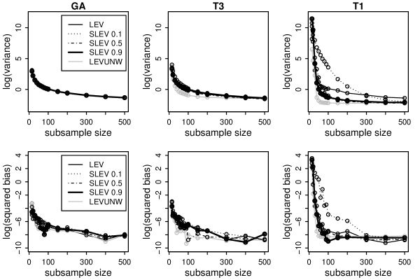
Figure 4: (Improvements from SLEV and LEVUNW subsection.) Comparison of variances and squared biases of the LEV, SLEV, and LEVUNW estimators in three data sets (GA, $T_{3}$, and $T_{1}$) for $n=1000$ and $p=10$. Left panels are GA data; Middle panels are $T_{3}$ data; Right panels are $T_{1}$ data. Grey lines are LEVUNW; black lines are LEV; dotted lines are SLEV with $\alpha=0.1$; dotdashed lines are SLEV with $\alpha=0.5$; thick black lines are SLEV with $\alpha=0.9$.

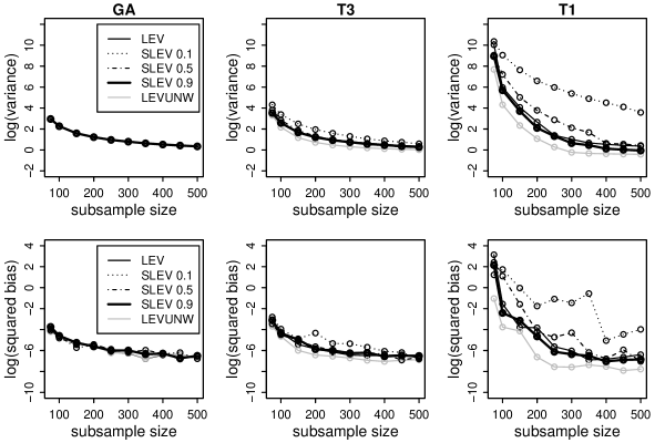
Figure 5: (Improvements from SLEV and LEVUNW subsection.) Same as Figure 4, except that $n=1000$ and $p=50$.

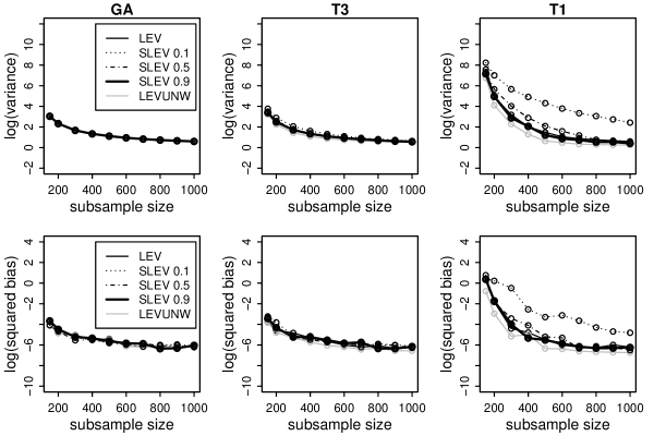
Figure 6: (Improvements from SLEV and LEVUNW subsection.) Same as Figure 4, except that $n=1000$ and $p=100$.

Consider Figures 4, 5, and 6, which present the variance and bias for synthetic data matrices (for GA, $T_{3}$, and $T_{1}$ data) of size $n\times p$, where $n=1000$ and $p=10$, $50$, and $100$, respectively. In each case, LEV, SLEV for three different values of the convex combination parameter $\alpha$, and LEVUNW were considered. Several observations are worth making. First of all, for GA data (left panel in these figures), all the results tend to be quite similar; but for $T_{3}$ data (middle panel) and even more so for $T_{1}$ data (right panel), differences appear. Second, SLEV with $\alpha\simeq 0.1$, i.e., when SLEV consists mostly of the uniform distribution, is notably worse in a manner similarly as with UNIF. Moreover, there is a gradual decrease in both bias and variance for our proposed SLEV as $\alpha$ is increased; and when $\alpha\simeq 0.9$ SLEV is slightly better than LEV. Finally, our proposed LEVUNW often has the smallest bias and variance over a wide range of subsample sizes for both $T_{3}$ and $T_{1}$, although the effect is not major. All in all, these observations are consistent with our main theoretical results.

Consider next Figure 7. This figure examines the optimal convex combination choice for $\alpha$ in SLEV, and $\alpha$ is the x-axis in all the plots. Different column panels in Figure 7 correspond to different subsample sizes $r$. Recall that there are two conflicting goals for SLEV: adding $(1-\alpha)/n$ to the small leverage scores will avoid substantially inflating the variance of the resulting estimate by samples with extremely small leverage scores; and doing so will lead to larger sample size $r$ in order to obtain bounds of the form Eqns. (8) and (9). Figure 7 plots the variance and bias for $T_{1}$ data for a range of parameter values and for a range of subsample sizes. In general, one sees that using SLEV to increase the probability of choosing small leverage components with $\alpha$ around $0.8-0.9$ (and relatedly shrinking the effect of large leverage components) has a beneficial effect on bias as well as variance. This is particularly true in two cases: first, when the matrix is very rectangular, e.g., when the $p=10$, which is consistent with the leverage score statistics from Table 1; and second, when the subsample size $r$ is larger, as the results for $r=3p$ are much choppier (and for $r=2p$, they are still choppier). As a rule of thumb, these plots suggest that choosing $\alpha=0.9$, and thus using $\pi_{i}=\alpha\pi^{Lev}_{i}+(1-\alpha)/n$ as the importance sampling probabilities, strikes a balance between needing more samples and avoiding variance inflation.

One can also see in Figure 7 the grey lines, dots, and dashes, which correspond to LEVUNW for the corresponding values of $p$, that LEVUNW consistently has smaller variances than SLEV for all values of $\alpha$. We should emphasize, though, that these are unconditional biases and variances. Since LEVUNW is approximately unbiased relative to the full sample weighted LS estimate $\hat{\boldsymbol{\beta}}_{wls}$, however, there is a large bias away from the full sample unweighted LS estimate $\hat{\boldsymbol{\beta}}_{ols}$. This suggests that LEVUNW may be used when the primary goal is to infer the true $\boldsymbol{\beta}_{0}$; but that when the primary goal is rather to approximate the full sample unweighted LS estimate, or when conditional biases and variances are of interest, then SLEV may be more appropriate. We will discuss this in greater detail in Section 4.4 next.

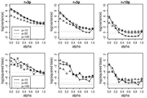
Figure 7: (Improvements from SLEV and LEVUNW subsection.) Varying $\alpha$ in SLEV. Comparison of variances and squared biases of the SLEV estimator in data generated from $T_{1}$ with $n=1000$ and variable $p$. Left panels are subsample size $r=3p$; Middle panels are $r=5p$; Right panels are $r=10p$. Circles connected by black lines are $p=10$; squares connected by dash lines are $p=50$; triangles connected by dotted lines are $p=100$. Grey corresponds to the LEVUNW estimator.

4.4 Conditional Bias and Variance

Here, we will describe the properties of the conditional bias and variance under various subsampling estimators. These will provide a more direct comparison with Eqns. (14) and (15) from Lemma 2 and the corresponding bounds from Lemma 6. These will also provide a more direct comparison with previous work that has adopted an algorithmic perspective on algorithmic leveraging [11, 27, 10].

Consider Figure 8, which presents our main empirical results for conditional biases and variances. As before, matrices were generated from GA, $T_{3}$ and $T_{1}$; and we calculated the empirical bias and variance of UNIF, LEV, SLEV with $\alpha=0.9$, and LEVUNW—in all cases, conditional on the empirical data $\boldsymbol{y}$. Several observations are worth making. First, for GA the variances are all very similar the same; and the biases are also, with the exception of LEVUNW. This is expected, since by the conditional expectation bounds from Lemma 6, LEVUNW is approximately unbiased, relative to the full sample weighted LS estimate $\hat{\boldsymbol{\beta}}_{wls}$—and thus there should be a large bias away from the full sample unweighted LS estimate. Second, for $T_{3}$ and even more prominently for $T_{1}$, the variance of LEVUNW is less than that for the other estimators. Third, when the leverage scores are very nonuniform, as with $T_{1}$, the relative merits of UNIF versus LEVUNW depend on the subsample size $r$. In particular, the bias of LEVUNW is larger than that of even UNIF for very aggressive downsampling; but it is substantially less than UNIF for moderate to large sample sizes.

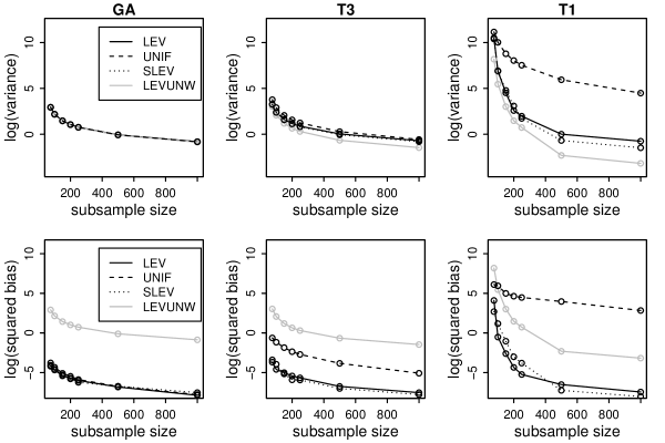
Figure 8: (Conditional Bias and Variance subsection.) Comparison of conditional variances and squared biases of the LEV and UNIF estimators in three data sets (GA, $T_{3}$, and $T_{1}$) for $n=1000$ and $p=50$. Left panels are GA data; Middle panels are $T_{3}$ data; Right panels are $T_{1}$ data. Upper panels are Variances; Lower panels are Squared Bias. Black lines for LEV estimate; dash lines for UNIF estimate; grey lines for LEVUNW estimate; dotted lines for SLEV estimate with $\alpha=0.9$.

Based on these and our other results, our default recommendation is to use SLEV (with either exact or approximate leverage scores) with $\alpha\approx 0.9$: it is no more than slightly worse than LEVUNW when considering unconditional biases and variances, and it can be much better than LEVUNW when considering conditional biases and variances.

5 Additional Empirical Evaluation

In this section, we provide additional empirical results (of a more specialized nature than those presented in Section 4). Here is a brief outline of the main results of this section.

• In Section 5.1, we will consider the synthetic data, and we will describe what happens when the subsampled problem looses rank. This can happen if one is extremely aggressive in downsampling with SLEV; but it is much more common with UNIF, even if one samples many constraints. In both cases, the behavior of bias and variance is very different than when rank is preserved.

• Then, in Section 5.2, we will summarize our results on synthetic data when the leverage scores are computed approximately with the fast approximation algorithm of [10]. Among other things, we will describe the running time of this algorithm, illustrating that it can solve larger problems than can be solved with traditional deterministic methods; and we will evaluate the unconditional bias and variance of SLEV when this algorithm is used to approximate the leverage scores.

• Finally, in Section 5.3, we will consider real data, and we will present our results for the conditional bias and variance for two data sets that are drawn from our previous work in two genetics applications. One of these has very uniform leverage scores, and the other has moderately nonuniform leverage scores; and our results from the synthetic data hold also in these realistic applications.

5.1 Leveraging and Uniform Estimates for Singular Subproblems

Here, we will describe the properties of LEV versus UNIF for situations in which rank is lost in the construction of the subproblem. That is, in some cases, the subsampled matrix, $X^{*}$, may have column rank that is smaller than the rank of the original matrix $X$, and this leads to a singular $X^{*T}X^{*}=X^{T}WX$. Of course, the LS solution of the subproblem can still be solved, but there will be a “bias” due to the dimensions that are not represented in the subsample. (We use the Moore-Penrose generalized inverse to compute the estimators when rank is lost in the construction of the subproblem.) Before describing these results, recall that algorithmic leveraging (in particular, LEV, but it holds for SLEV as well) guarantees that this will not happen in the following sense: if roughly $O(p\log p)$ rows of $X$ are sampled using an importance sampling distribution that approximates the leverage scores in the sense of Eqn. (7), then with very high probability the matrix $X^{*}$ does not loose rank [11, 27, 10]. Indeed, this observation is crucial from the algorithmic perspective, i.e., in order to obtain relative-error bounds of the form of Eqns. (8) and (9), and thus it was central to the development of algorithmic leveraging. On the other hand, if one downsamples more aggressively, e.g., if one samples only, say, $p+100$ or $p+10$ rows, or if one uses uniform sampling when the leverage scores are very nonuniform, then it is possible to loose rank. Here, we examine the statistical consequences of this.

We have observed this phenomenon with the synthetic data for both UNIF as well as for leverage-based sampling procedures; but the properties are somewhat different depending on the sampling procedure. To illustrate both of these with a single synthetic example, we first generated a $1000\times 10$ matrix from multivariate $t$-distribution with $3$ (or $2$ or $1$, denoted $T_{3}$, $T_{2}$, and $T_{1}$, respectively) degrees of freedom and covariance matrix $\Sigma_{ij}=2\times 0.5^{|i-j|}$; we then calculated the leverage scores of all rows; and finally we formed the matrix $X$ was by keeping the $50$ rows with highest leverage scores and replicating $950$ times the row with the smallest leverage score. (This is a somewhat more realistic version of the toy Worst-case Matrix that is described in Section A.2.) We then applied LEV and UNIF to the data sets with different subsample sizes, as we did for the results summarized in Section 4.2. Our results are summarized in Figure 9 and 10.

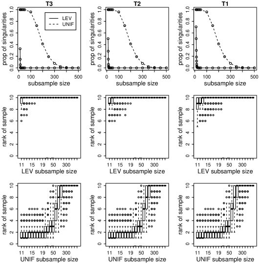
Figure 9: Comparison of LEV and UNIF when rank is lost in the sampling process ($n=1000$ and $p=10$ here). Left panels are $T_{3}$; Middle panels are $T_{2}$; Right panels are $T_{1}$. Upper panels are proportion of singular $X^{T}WX$, out of $500$ trials, for both LEV (solid lines) and UNIF (dashed lines); Middle panels are boxplots of ranks of $500$ LEV subsamples; Lower panels are boxplots of ranks of $500$ UNIF subsamples. Note the nonstandard scaling of the X axis.

Figure 10: Comparison of LEV and UNIF when rank is lost in the sampling process ($n=1000$ and $p=10$ here). Left panel are $T_{3}$; Middle panels are $T_{2}$; Right panels are $T_{1}$. Upper panels are logarithm of variances of the estimates; Middle panels are logarithm of variances, zoomed-in on the X-axis; Lower panels are logarithm of squared bias of the estimates. Black line for LEV; Dash line for UNIF.

The top row of Figure 9 plots the fraction of singular $X^{T}WX$, out of $500$ trials, for both LEV and UNIF; from left to right, results for $T_{3}$, $T_{2}$, and $T_{1}$ are shown. Several points are worth emphasizing. First, both LEV and UNIF loose rank if the downsampling is sufficiently aggressive. Second, for LEV, as long as one chooses more than roughly $20$ (or less for $T_{2}$ and $T_{1}$), i.e., the ratio $r/p$ is at least roughly $2$, then rank is not lost; but for uniform sampling, one must sample a much larger fraction of the data. In particular, when fewer than $r=100$ samples are drawn then nearly all of the subproblems constructed with the UNIF procedure are singular, and it is not until more than $r=300$ that nearly all of the subproblems are not singular. Although these particular numbers depend on the particular data, needing to draw many more samples with UNIF than with LEV in order to preserve rank is a very general phenomenon. The middle row of Figure 9 shows the boxplots of rank for the subproblem for LEV for those $500$ tries; and the bottom row shows the boxplots of the rank of the subproblem for UNIF for those $500$ tries. Note the unusual scale on the X-axis designed to highlight the lost rank data for both LEV as well as UNIF. These boxplots illustrate the sigmoidal distribution of ranks that obtained by UNIF as a function of the number of samples and the less severe beginning of the sigmoid for LEV; and they also show that when subproblems are singular, then often many dimensions fail to be captured. All in all, LEV outperforms UNIF, especially when the leverage scores are nonuniform.

Figure 10 illustrates the variance and bias of the corresponding estimators. In particular, the upper panels plot the logarithm of variances; the middle panels plot the same quantities, except that it is zoomed-in on the X-axis; and the lower panels plot the logarithm of squared bias. As before, the left/middle/right panels present results for the $T_{3}$/$T_{2}$/$T_{1}$ data, respectively. The behavior here is very different that that shown in Figures 1, 2, and 3; and several observations are worth making. First, for all three models and for both LEV and UNIF, when the downsampling is very aggressive, e.g, $r=p+5$ or $r=p+10$, then the bias is comparable to the variance. That is, since the sampling process has lost dimensions, the linear approximation implicit in our Taylor expansion is violated. Second, both bias and variance are worse for $T_{1}$ than for $T_{2}$ than for $T_{3}$, which is consistent with Table 1, but the effect is minor; and the bias and variance are generally much worse for UNIF than for LEV. Third, as $r$ increases, the variance for UNIF increases, hits a maximum and then decreases; and at the same time the bias for UNIF gradually decreases. Upon examining the original data, the reason that there is very little variance initially is that most of the subsamples have rank $1$ or $2$; then the variance increases as the dimensionality of the subsamples increases; and then the variance decreases due to the $1/r$ scaling, as we saw in the plots in Section 4.2. Fourth, as $r$ increases, both the variance and bias of LEV decrease, as we saw in Section 4.2; but in the aggressive downsampling regime, i.e., when $r$ is very small, the variance of LEV is particularly “choppy,” and is actually worse than that of UNIF, perhaps also due to rank deficiency issues.

5.2 Approximate Leveraging via the Fast Leveraging Algorithm

Here, we will describe using the fast randomized algorithm from [10] to compute approximations to the leverage scores of $X$, to be used in place of the exact leverage scores in LEV, SLEV, and LEVUNW. To start, we provide a brief description of the algorithm of [10], which takes as input an arbitrary $n\times p$ matrix $X$.

• Generate an $r_{1}\times n$ random matrix $\Pi_{1}$ and a $p\times r_{2}$ random matrix $\Pi_{2}$.

• Let $R$ be the $R$ matrix from a QR decomposition of $\Pi_{1}X$.

• Compute and return the leverage scores of the matrix $XR^{-1}\Pi_{2}$.

For appropriate choices of $r_{1}$ and $r_{2}$, if one chooses $\Pi_{1}$ to be a Hadamard-based random projection matrix, then this algorithm runs in $o(np^{2})$ time, and it returns $1\pm\epsilon$ approximations to all the leverage scores of $X$ [10]. In addition, with a high-quality implementation of the Hadamard-based random projection, this algorithm runs faster than traditional deterministic algorithms based on Lapack for matrices as small as several thousand by several hundred [3, 17].

We have implemented in the software environment R two variants of this fast algorithm of [10], and we have compared it with QR-based deterministic algorithms also supported in R for computing the leverage scores exactly. In particular, the following results were obtained on a PC with Intel Core i7 Processor and 6 Gbytes RAM running Windows 7, on which we used the software package R, version 2.15.2. In the following, we refer to the above algorithm as BFast (the Binary Fast algorithm) when (up to normalization) each element of $\Pi_{1}$ and $\Pi_{2}$ is generated i.i.d. from $\{-1,1\}$ with equal sampling probabilities; and we refer to the above algorithm as GFast (the Gaussian Fast algorithm) when each element of $\Pi_{1}$ is generated i.i.d. from a Gaussian distribution with mean zero and variance $1/n$ and each element of $\Pi_{2}$ is generated i.i.d. from a Gaussian distribution with mean zero and variance $1/p$. (In particular, note that here we do not consider Hadamard-based projections for $\Pi_{1}$ or more sophisticated parallel and distributed implementations of these algorithms [3, 30, 17, 44].)

To illustrate the behavior of this algorithm as a function of its parameters, we considered synthetic data where the $20,000\times 1,000$ design matrix $X$ is generated from $T_{1}$ distribution. All the other parameters are set to be the same as before, except $\Sigma_{ij}=0.1$, for $i\neq j$, and $\Sigma_{ii}=2$. We then applied BFast and GFast with varying $r_{1}$ and $r_{2}$ to the data. In particular, we set $r_{1}=p,1.5p,2p,3p,5p$, where $p=1,000$, and we set $r_{2}=\kappa\log(n)$, for $\kappa=1,2,3,4,5,10,20$, where $n=20,000$. See Figure 11, which presents both a summary of the correlation between the approximate and exact leverage scores as well as a summary of the running time for computing the approximate leverage scores, as $r_{1}$ and $r_{2}$ are varied for both BFast and GFast. We can see that the correlations between approximated and exact leverage scores are not very sensitive to varying $r_{1}$, whereas the running time increases roughly linearly for increasing $r_{1}$. In contrast, the correlations between approximated and exact leverage scores increases rapidly for increasing $r_{2}$, whereas the running time does not increase much when $r_{2}$ increases. These observations suggest that we may use a combination of small $r_{1}$ and large $r_{2}$ to achieve high-quality approximation and short running time.

Figure 11: (Fast Leveraging Algorithm subsection.) Effect of approximating leverage scores using BFast and GFast for varying parameters. Upper panels: Varying parameter $r_{1}$ for fixed $r_{2}$, where $r_{2}=\log(n)$ (black lines), $r_{2}=5\log(n)$ (dashed lines), and $r_{2}=10\log(n)$ (dotted lines). Lower panels: Varying parameter $r_{2}$ for fixed $r_{1}$, where $r_{1}=p$ (black lines), $r_{1}=3p$ (dashed lines), and $r_{1}=5p$ (dotted lines). Left two panels: Correlation between exact leverage scores and leverage scores approximated using BFast and GFast, for varying $r_{1}$ and $r_{2}$. Right two panels: CPU time for varying $r_{1}$ and $r_{2}$, using BFast and GFast.

Next, we examine the running time of the approximation algorithms for computing the leverage scores. Our results for running times are summarized in Figure 12. In that figure, we plot the running time as sample size $n$ and predictor size $p$ are varied for BFast and GFast. We can see that when the sample size is very small, the computation time of the fast algorithms is slightly worse than that of the exact algorithm. (This phenomenon is primarily since the fast algorithm requires additional projection and matrix multiplication steps, which dominate the running time for very small matrices.) On the other hand, when the sample size is larger than ca. $20,000$, the computation time of the fast approximation algorithms becomes slightly less expensive than that of exact algorithm. Much more significantly, when the sample size is larger than roughly $35,000$, the exact algorithm requires more memory than our standard R environment can provide, and thus it fails to run at all. In contrast, the fast algorithms can work with sample size up to roughly $60,000$.

That is, the use of this randomized algorithm to approximate the leverage scores permits us to work with data that are roughly $1.5$ times larger in $n$ or $p$, even when a simple vanilla implementation is provided in the R environment. (If one is interested in much larger inputs, e.g., with $n=10^{6}$ or more, then one should probably not work within R and instead use Hadamard-based random projections for $\Pi_{1}$ and/or the use of more sophisticated methods, such as those described in [3, 30, 17, 44]; here we simply evaluate an implementation of these methods in R.) The reason that BFast and GFast can run for much larger input is likely that the computational bottleneck for the exact algorithm is a QR decomposition, while the computational bottleneck for the fast randomized algorithms is the matrix-matrix multiplication step.

Figure 12: (Fast Leveraging Algorithm subsection.) CPU time for calculating exact leverage scores and approximate leverage scores using the BFast and GFast versions of the fast algorithm of [10]. Left panel is CPU time for varying sample size $n$ for fixed predictor size $p=500$; Right panel is CPU time for varying predictor size $p$ for fixed sample size $n=2000$. Black lines connect the CPU time for calculating exact leverage scores; dash lines connect the CPU time for using GFast to approximate the leverage scores; dotted lines connect the CPU time for using BFast to approximate the leverage scores.

Finally, we evaluate the bias and variance of LEV, SLEV and LEVUNW estimates where the leverage scores are calculated using exact algorithm, BFast, and GFast. In Figure 13, we plot the variance and squared bias for $T_{3}$ data sets. (We have observed similar but slightly smoother results for the Gaussian data sets and similar but slightly choppier results for the $T_{1}$ data sets.) Observe that the variances of LEV estimates where the leverage scores are calculated using exact algorithm, BFast, and GFast are almost identical; and this observation is also true for SLEV and LEVUNW estimates. All in all, using the fast approximation algorithm of [10] to compute approximations to the leverage scores for use in LEV, SLEV, and LEVUNW leads to improved algorithmic performance, while achieving nearly identical statistical results as LEV, SLEV, and LEVUNW when the exact leverage scores are used.

Figure 13: (Fast Leveraging Algorithm subsection.) Comparison of variances and squared biases of the LEV, SLEV, and LEVUNW estimators in $T_{3}$ data sets for $n=20000$ and $p=5000$ using BFast and GFast versions of the fast algorithm of [10]. Left panels are LEV estimates; Middle panels are SLEV estimates; Right panels are LEVUNW estimates. Black lines are exact algorithm; dash lines are BFast; dotted lines are GFast.

5.3 Illustration of the Method on Real Data

Here, we provide an illustration of our methods on two real data sets drawn from two problems in genetics with which we have prior experience [9, 28]. The first data set has relatively uniform leverage scores, while the second data set has somewhat more nonuniform leverage scores. These two examples simply illustrate that observations we made on the synthetic data also hold for more realistic data that we have studied previously. For more information on the application of these ideas in genetics, see previous work on PCA-correlated SNPs [35, 34].

5.3.1 Linear model for bias correction in RNA-Seq data

In order to illustrate how our methods perform on a real data set with nearly uniform leverage scores, we consider an RNA-Seq data set containing $n=51,751$ read counts from embryonic mouse stem cells [15]. Recall that RNA-Seq is becoming the major tool for transcriptome analysis; it produces digital signals by obtaining tens of millions of short reads; and after being mapped to the genome, RNA-Seq data can be summarized by a sequence of short-read counts. Recent work found that short-read counts have significant sequence bias [25]. Here, we consider a simplified linear model of [9] for correcting sequence bias in RNA-Seq. Let $n_{ij}$ denote the counts of reads that are mapped to the genome starting at the $j$th nucleotide of the $i$th gene, where $i=1,2,\ldots,100$ and $j=1,\ldots,L_{i}$. We assume that the log transformed count of reads, $y_{ij}=\log(n_{ij}+0.5)$, depends on $40$ nucleotides in the neighborhood, denoted as $b_{ij,-20},b_{ij,-19},\ldots,b_{ij,18},b_{ij,19}$ through the following linear model: $y_{ij}=\alpha+\sum_{k=-20}^{19}\sum_{h\in\cal{H}}\beta_{kh}I(b_{ij,k}=h)+\epsilon_{ij},$ where ${\cal{H}}=\{A,C,G\}$, where $T$ is used as the baseline level, $\alpha$ is the grand mean, $I(b_{ij,k}=h)$ equals to 1 if the $k$th nucleotide of the surrounding sequence is $h$, and $0$ otherwise, $\beta_{kh}$ is the coefficient of the effect of nucleotide $h$ occurring in the $k$th position, and $\epsilon_{ij}\sim N(0,\sigma^{2})$. This linear model uses $p=121$ parameters to model the sequence bias of read counts. For $n=51,751$, model-fitting via LS is time-consuming.

Coefficient estimates were obtained using three subsampling algorithms for seven different subsample sizes: $2p,3p,4p,5p,10p,20p,50p$. We compare the estimates using the sample bias and variances; and, for each subsample size, we repeat our sampling $100$ times to get $100$ estimates. (At each subsample size, we take one hundred subsamples and calculate all the estimates; we then calculate the bias of the estimates with respect to the full sample least squares estimate and their variance.) See Figure 14 for a summary of our results. In the left panel of Figure 14, we plot the histogram of the leverage score sampling probabilities. Observe that the distribution is quite uniform, suggesting that leverage-based sampling methods will perform similarly to uniform sampling. To demonstrate this, the middle and right panels of Figure 14 present the (conditional) empirical variances and biases of each of the four estimates, for seven different subsample sizes. Observe that LEV, LEVUNW, SLEV, and UNIF all have comparable sample variances. When the subsample size is very small, all four methods have comparable sample bias; but when the subsample size is larger, then LEVUNW has a slightly larger bias than the other three estimates.

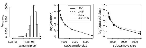
Figure 14: Empirical results for real data. Left panel is the histogram of the leverage score sampling probabilities for the RNA-Seq data (the largest leverage score is $2.25\times 10^{-5}$, and the mean is $1.93\times 10^{-5}$, i.e., the largest is only slightly larger than the mean); Middle panel is the empirical conditional variances of the LEV, UNIF, LEVUNW, and SLEV estimates; Right panel is the empirical conditional biases. Black lines for LEV; dash lines for UNIF; grey lines for LEVUNW; dotted lines for SLEV with $\alpha=0.9$.

5.3.2 Linear model for predicting gene expressions of cancer patient

In order to illustrate how our methods perform on real data with moderately nonuniform leverage scores, we consider a microarray data set that was presented in [33] (and also considered in [28]) for $46$ cancer patients with respect to $n=5,520$ genes. Here, we randomly select one patient’s gene expression as the response $\boldsymbol{y}$ and use the remaining patients’ gene expressions as the predictors (so $p=45$); and we predict the selected patient’s gene expression using other patients gene expressions through a linear model. We fit the linear model using subsampling algorithms with nine different subsample sizes. See Figure 15 for a summary of our results. In the left panel of Figure 15, we plot the histogram of the leverage score sampling probabilities. Observe that the distribution is highly skewed and quite a number of probabilities are significantly larger than the average probability. Thus, one might expect that leveraging estimates will have an advantage over the uniform sampling estimate. To demonstrate this, the middle and right panels of Figure 15 present the (conditional) empirical variances and biases of each of the four estimates, for nine different subsample sizes. Observe that SLEV and LEV have smaller sample variance than LEVUNW and that UNIF consistently has the largest variance. Interestingly, since LEVUNW is approximately unbiased to the weighted least squares estimate, here we observe that LEVUNW has by far the largest bias and that the bias does not decrease as the subsample size increases. In addition, when the subsample size is less than 2000, the biases of LEV, SLEV and UNIF are comparable; but when the subsample size is greater than 2000, LEV and SLEV have slightly smaller bias than UNIF.

Figure 15: Empirical results for real data. Left panel is the histogram of the leverage score sampling probabilities for the microarray data (the largest leverage score is $0.00124$, and the mean is $0.00018$, i.e., the largest is $7$ times the mean); Middle panel is the empirical conditional variances of the LEV, UNIF, LEVUNW, and SLEV estimates; Right panel is the empirical conditional biases. Black lines for LEV; dash lines for UNIF; grey lines for LEVUNW; dotted lines for SLEV with $\alpha=0.9$.

6 Discussion and Conclusion

Algorithmic leveraging—a recently-popular framework for solving large least-squares regression and other related matrix problems via sampling based on the empirical statistical leverage scores of the data—has been shown to have many desirable algorithmic properties. In this paper, we have adopted a statistical perspective on algorithmic leveraging, and we have demonstrated how this leads to improved performance of this paradigm on real and synthetic data. In particular, from the algorithmic perspective of worst-case analysis, leverage-based sampling provides uniformly superior worst-case algorithmic results, when compared with uniform sampling. Our statistical analysis, however, reveals that, from the statistical perspective of bias and variance, neither leverage-based sampling nor uniform sampling dominates the other. Based on this, we have developed new statistically-inspired leveraging algorithms that achieve improved statistical performance, while maintaining the algorithmic benefits of the usual leverage-based method. Our empirical evaluation demonstrates that our theory is a good predictor of the practical performance of both existing as well as our newly-proposed leverage-based algorithms. In addition, our empirical evaluation demonstrates that, by using a recently-developed algorithm to approximate the leverage scores, we can compute improved approximate solutions for much larger least-squares problems than we can compute the exact solutions with traditional deterministic algorithms.

Finally, we should note that, while our results are straightforward and intuitive, obtaining them was not easy, in large part due to seemingly-minor differences between problem formulations in statistics, computer science, machine learning, and numerical linear algebra. Now that we have “bridged the gap” by providing a statistical perspective on a recently-popular algorithmic framework, we expect that one can ask even more refined statistical questions of this and other related algorithmic frameworks for large-scale computation.

Appendix A Asymptotic Analysis and Toy Data

In this section, we will relate our analytic methods to the notion of asymptotic relative efficiency, and we will consider several toy data sets that illustrate various aspects of algorithmic leveraging. Although the results of this section are not used elsewhere, and thus some readers may prefer skip this section, we include it in order to relate our approach to ideas that may be more familiar to certain readers.

A.1 Asymptotic Relative Efficiency Analysis

Here, we present an asymptotic analysis comparing UNIF with LEV, SLEV, and LEVUNW in terms of their relative efficiency. Recall that one natural way to compare two procedures is to compare the sample sizes at which the two procedures meet a given standard of performance. One such standard is efficiency, which addresses how “spread out” about $\boldsymbol{\beta}_{0}$ is the estimator. In this case, the smaller the variance, the more “efficient” is the estimator [38]. Since $\boldsymbol{\beta}_{0}$ is a $p$-dimensional vector, to determine the relative efficiency of two estimators, we consider the linear combination of $\boldsymbol{\beta}_{0}$, i.e., $c^{T}\boldsymbol{\beta}_{0}$, where $c$ is the linear combination coefficient. In somewhat more detail, when $\hat{\boldsymbol{\beta}}$ and $\tilde{\boldsymbol{\beta}}$ are two one-dimensional estimates, their relative efficiency can be defined as

$$e(\hat{\boldsymbol{\beta}},\tilde{\boldsymbol{\beta}})=\frac{\text{Var}(\tilde{\boldsymbol{\beta}})}{\text{Var}(\hat{\boldsymbol{\beta}})},$$

and when $\hat{\boldsymbol{\beta}}$ and $\tilde{\boldsymbol{\beta}}$ are two $p$-dimensional estimates, we can take their linear combinations $c^{T}\hat{\boldsymbol{\beta}}$ and $c^{T}\tilde{\boldsymbol{\beta}}$, where $c$ is the linear combination coefficient vector, and define their relative efficiency as

$$e(c^{T}\hat{\boldsymbol{\beta}},c^{T}\tilde{\boldsymbol{\beta}})=\frac{\text{Var}(c^{T}\tilde{\boldsymbol{\beta}})}{\text{Var}(c^{T}\hat{\boldsymbol{\beta}})}.$$

In order to discuss asymptotic relative efficiency, we start with the following seemingly-technical observation.

Definition 1.

A $k\times k$ matrix A is said to be $A=O(\alpha_{n})$ if and only if every element of $A$ satisfies $A_{ij}=O(\alpha_{n})$ for $i,j=1,\ldots,k$.

Assumption 1.

$X^{T}X=\sum_{i=1}^{n}\boldsymbol{x}_{i}\boldsymbol{x}_{i}^{T}$ is positive definite and $(X^{T}X)^{-1}=O(\alpha_{n}^{-1})$.

Remark. Assuming $X^{T}X$ is nonsingular, for a LS estimator $\hat{\boldsymbol{\beta}}_{ols}$ to converge to true value $\boldsymbol{\beta}_{0}$ in probability, it is sufficient and necessary that $(X^{T}X)^{-1}\rightarrow 0$ as $n\rightarrow\infty$ [2, 24].

Remark. Although we have stated this as an assumption, one typically assumes an $n$-dependence for $\alpha_{n}$ [2]. Since the form of the $n$-dependence is unspecified, we can alternatively view Assumption 1 as a definition of $\alpha_{n}$. The usual assumption that is made (typically for analytical convenience) is that $\alpha_{n}=n$ [16]. We will provide examples of toy data for which $\alpha_{n}=n$, as well as examples for which $\alpha_{n}\neq n$. In light of our empirical results in Section 4 and the empirical observation that leverage scores are often very nonuniform [28, 17], it is an interesting question to ask whether the common assumption that $\alpha_{n}=n$ is too restrictive, e.g., whether it excludes interesting matrices $X$ with very heterogeneous leveraging scores.

Under Assumption 1, i.e., that $(X^{T}X)^{-1}$ is asymptotically parameterized as $(X^{T}X)^{-1}=O(\alpha_{n}^{-1})$, we have the following three results to compare the leveraging estimators and the uniform sampling estimator. The expressions in these three lemmas are complicated; and, since they are expressed in terms of $\alpha_{n}$, they are not easy to evaluate on real or synthetic data. (It is partly for this reason that our empirical evaluation is in terms of the bias and variance of the subsampling estimators.) We start by stating a lemma characterizing the relative efficiency of LEV and UNIF; the proof of this lemma may be found in Appendix B.5.

Lemma 7.

To leading order, the asymptotic relative efficiency of $c^{T}\tilde{\boldsymbol{\beta}}_{LEV}$ and $c^{T}\tilde{\boldsymbol{\beta}}_{UNIF}$ is

$$e(c^{T}\tilde{\boldsymbol{\beta}}_{LEV},c^{T}\tilde{\boldsymbol{\beta}}_{UNIF})\simeq O(\frac{\frac{1}{\alpha_{n}}+\frac{1}{{r}}\sqrt{\sum_{i}(1-h_{ii})^{4}\max(h_{ii})}}{\frac{1}{\alpha_{n}}+\frac{1}{{\alpha_{n}r}}\sqrt{\sum_{i}\frac{(1-h_{ii})^{4}}{h_{ii}^{2}}\max(h_{ii})}}),$$ (24)

where the residual variance is ignored.

Next, we state a lemma characterizing the relative efficiency of SLEV and UNIF; the proof of this lemma is similar to that of Lemma 7 and is thus omitted.

Lemma 8.

To leading order, the asymptotic relative efficiency of $c^{T}\tilde{\boldsymbol{\beta}}_{SLEV}$ and $c^{T}\tilde{\boldsymbol{\beta}}_{UNIF}$ is

$$e(c^{T}\tilde{\boldsymbol{\beta}}_{SLEV},c^{T}\tilde{\boldsymbol{\beta}}_{UNIF})\simeq O(\frac{\frac{1}{\alpha_{n}}+\frac{1}{{r}}\sqrt{\sum_{i}(1-h_{ii})^{4}\max(h_{ii})}}{\frac{1}{\alpha_{n}}+\frac{1}{{\alpha_{n}r}}\sqrt{\sum_{i}\frac{(1-h_{ii})^{4}}{\pi_{i}^{2}}\max(h_{ii})}}),$$

where the residual variance is ignored.

Finally, we state a lemma characterizing the relative efficiency of LEVUNW and UNIF; the proof of this lemma may be found in Appendix B.6.

Lemma 9.

To leading order, the asymptotic relative efficiency of $c^{T}\tilde{\boldsymbol{\beta}}_{LEVUNW}$ and $c^{T}\tilde{\boldsymbol{\beta}}_{UNIF}$ is

$$e(c^{T}\tilde{\boldsymbol{\beta}}_{LEVUNW},c^{T}\tilde{\boldsymbol{\beta}}_{UNIF})\simeq O(\frac{\frac{1}{\alpha_{n}}+\frac{1}{{r}}\sqrt{\sum_{i}(1-h_{ii})^{4}\max(h_{ii})}}{\frac{\max(h_{ii})}{\alpha_{n}\min(h_{ii})}+\frac{1}{{\alpha_{n}\min(h_{ii})r}}\sqrt{\sum_{i}(1-g_{ii})^{4}\max(g_{ii})}}),$$

where the residual variance is ignored and $g_{ii}=h_{ii}\boldsymbol{x}_{i}^{T}(X^{T}\mbox{}{Diag}\left\{h_{ii}\right\}X)^{-1}\boldsymbol{x}_{i}$.

Of course, in an analogous manner, one could derive expressions for the asymptotic relative efficiencies $e(c^{T}\tilde{\boldsymbol{\beta}}_{SLEV},c^{T}\tilde{\boldsymbol{\beta}}_{LEV})$, $e(c^{T}\tilde{\boldsymbol{\beta}}_{LEVUNW},c^{T}\tilde{\boldsymbol{\beta}}_{LEV})$, and $e(c^{T}\tilde{\boldsymbol{\beta}}_{LEVUNW},c^{T}\tilde{\boldsymbol{\beta}}_{SLEV})$.

A.2 Illustration of the Method on Toy Data

Here, we will consider several toy data sets that illustrate various aspects of algorithmic leveraging, including various extreme cases of the method. While some of these toy data may seem artificial or contrived, they will highlight properties that manifest themselves in less extreme forms in the more realistic data in Section 4. Since the leverage score structure of the matrix $X$ is crucial for the behavior of the method, we will focus primarily on that structure. To do so, consider the two extreme cases. At one extreme, when the leverage scores are all equal, i.e., $h_{ii}=p/n$, for all $i\in[n]$, the first two variance terms in Eqn. (20) are equal to the first two variance terms in Eqn. (18). In this case, LEV simply reduces to UNIF. At the other extreme, the leverage scores can be very nonuniform—e.g., there can be a small number of leverage scores that are much larger than the rest and/or there can be some leverage scores that are much smaller than the mean score. Dealing with these two cases properly is crucial for the method of algorithmic leveraging, but these two cases highlight important differences between the more common algorithmic perspective and our more novel statistical perspective.

The former problem (of a small number of very large leverage scores) is of particular importance from an algorithmic perspective. The reason is that in that case one wants to compare the output of the sampling algorithm with the optimum based on the empirical data (as opposed to the “ground truth” solution). Thus, dealing with large leverage scores was a main issue in the development of the leveraging paradigm [11, 27, 10]. On the other hand, the latter problem (of some very small leverage scores) is also an important concern if we are interested in statistical properties of algorithmic leveraging. To see why, consider, e.g., the extreme case that a few data points have very very small leverage scores, e.g. $h_{ii}=1/n^{4}$ for some $i$. In this case, e.g., the second variance term in Eqn. (18) will be much larger than the second variance term in Eqn. (20).

In light of this discussion, here are several toy examples to consider. We will start with several examples where $p=1$ that illustrate things in the simplest setting.

• Example 1A: Sample Mean. Let $n$ be arbitrary, $p=1$, and let the $n\times p$ matrix $X$ be such that $X_{i}=1$, for all $i\in[n]$, i.e., let $X$ be the all-ones vector. In this case, $X^{T}X=n$ and $h_{ii}=1/n$, for all $i\in[n]$, i.e., the leverage scores are uniform, and thus algorithmic leveraging reduces to uniform sampling. Also, in this case, $\alpha_{n}=n$ in Assumption 1. All three asymptotic efficiencies are equal to $O(1)$.

• Example 1B: Simple Linear Combination. Let $n$ be arbitrary, $p=1$, and let the $n\times p$ matrix $X$ be such that $X_{i}=\pm 1$, for all $i\in[n]$, either uniformly at random, or such that $X_{i}=+1$ if $i$ is odd and $X_{i}=-1$ if $i$ is even. In this case, $X^{T}X=n$ and $h_{ii}=1/n$, for all $i\in[n]$, i.e., the leverage scores are uniform; and, in addition, $\alpha_{n}=n$ in Assumption 1. For all four estimators, all four unconditional variances are equal to $\sigma^{2}\{\frac{1}{n}+\frac{(1-1/n)^{2}}{r}\}$. In addition, for all four estimators, all three relative efficiencies are equal to $O(1)$.

• Example 2: “Inflated” Regression Line Through Origin. Let $n$ be arbitrary, $p=1$, and let the $n\times p$ matrix $X$ be such that $X_{i}=i$, i.e., they are evenly spaced and increase without limit with increasing $i$. (We thus refer the $X$ as “inflated.”) In this case,

  $$X^{T}X=n(n+1)(2n+1)/6,$$

  and the leverage scores equal

  $$h_{ii}=\frac{6i^{2}}{n(n+1)(2n+1)},$$

  i.e., the leverage scores $h_{ii}$ are very nonuniform. This is illustrated in the left panel of Figure 16. Also, in this case, $\alpha_{n}=n^{3}$ in Assumption 1. It is easy to see that the first variance components of UNIF, LEV, SLEV are the same, i.e., they equal

  $$(X^{T}X)^{-1}=\frac{6}{n(n+1)(2n+1)}.$$

  It is also easy to see that variances of LEV, SLEV and UNIF are dominated by their second variance component. The leading terms of the second variance component of LEV and UNIF are the same, and we expect to see the similar performance based on their variance. The leading term of the second variance component of SLEV is smaller than that of LEV and UNIF; and thus SLEV has smaller variance than LEV and UNIF. Simple calculation shows that LEVUNW has a smaller leading term for the second variance component than those of LEV, UNIF and SLEV.

• Example 3: “In-fill” Regression Line Through Origin. Let $n$ be arbitrary, $p=1$, and let the $n\times p$ matrix $X$ be such that $X_{i}=1/i$. This is different than the evenly spaced data points in the “inflated” toy example since the unevenly spaced data points this this example get denser in the interval $(0,1]$. The asymptotic properties of such design matrix are so-called “in-fill” asymptotics [8]. In this case,

  $$X^{T}X=\pi^{2}/6-\psi^{(1)}(n+1),$$

  where $\psi^{(k)}$ is the $k^{th}$ derivative of digamma function, and the leverage scores equal

  $$h_{ii}=\frac{1}{i^{2}(\pi^{2}/6-\psi^{(1)}(n+1))},$$

  i.e., the leverage scores $h_{ii}$ are very nonuniform. This is illustrated in the middle panel of Figure 16. Also, in this case, $\alpha_{n}=1$ in Assumption 1.

To obtain an improved understanding of these examples, consider the first two panels of Figures 16 and 17. Figure 16 shows the sampling probabilities for the Inflated Regression Line and the In-fill Regression Line. Both the Inflated Regression Line and the In-fill Regression Line have very nonuniform leverage scores, and by construction there is a natural ordering such that the leverage scores increase or decrease respectively. For the Inflated Regression Line, the minimum, mean, and maximum leverage scores are $6/(n(n+1)(2n+1))$, $1/n$, and $6n/(n+1)(2n+1)$, respectively; and for the In-fill Regression Line, the minimum, mean, and maximum leverage scores are $1/(n^{2}(\pi^{2}/6-\psi^{(1)}(n+1)))$, $1/n$, and $1/(\pi^{2}/6-\psi^{(1)}(n+1))$, respectively. For reference, note that for the Sample Mean (as well as for the Simple Linear Combination) all of the the leverage scores are equal to $1/n$, which equals $0.1$ for the value of $n=10$ used in Figure 16.

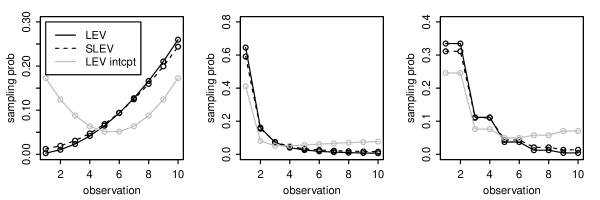
Figure 16: Leverage score-based sampling probabilities for three toy examples (Example 2, Example 3, and Example 4). Left panel is Inflated Regression Line (Example 2); Middle panel is In-fill Regression Line (Example 3); Right panel is Regression Surface (Example 4). In this example, we set $n=10$. Black lines connect the sampling probability for each data points for LEV; dash lines (below black) connect sampling probability for SLEV; and grey lines connect sampling probability for LEV after we add an intercept (i.e., the sample mean) as a second column to $X$.

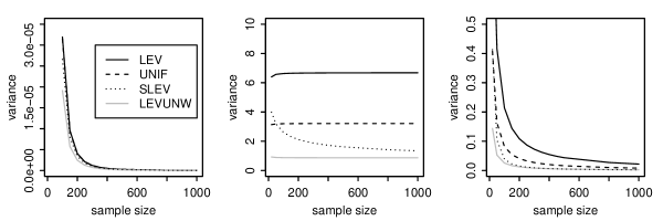
Figure 17: Theoretical variances for three toy examples (Example 2, Example 3, and Example 4) for various sample sizes $n$. Left panel is Inflated Regression Line (Example 2); Middle panel is In-fill Regression Line (Example 3); Right panel is Regression Surface (Example 4). In this example, we set $\sigma^{2}=1$ and $r=0.1n$, for varying $n$ from $100$ to $1000$. Black line for LEV (Equation 18); dash line for UNIF (Equation 20); dotted line (below black) for SLEV; and grey line for LEVUNW (Equation 23).

Figure 17 illustrates the theoretical variances for the same examples for particular values of $\sigma^{2}$ and $r$. In particular, observe that for the Inflated Regression Line, all three sampling methods tend to have smaller variance as $n$ is increased for a fixed value of $p$. This is intuitive, and it is a common phenomenon that we observe in most of the synthetic and real data sets. The property of the In-fill Regression Line where the variances are roughly flat (actually, they increase slightly) is more uncommon, but it illustrates that other possibilities exist. The reason is that leverage scores of most data points are relatively homogeneous (as long as $i$ is greater than $\sqrt{6n/\pi^{2}}$, the leverage score of $i$th observation is less than mean $1/n$ but greater than $1/n^{2}(\pi^{2}/6)$). When subsample size $r$ is reasonably large, we have high probabilities to sample these data points, whose sample probabilities inflate the variance. These curves also illustrate that LEV and UNIF can be better or worse with respect to each other, depending on the problem parameters; and that SLEV and LEVUNW can be better than either, for certain parameter values.

From these examples, we can see that the variance for the leveraging estimate can be inflated by very small leverage scores. That is, since the variances involve terms that depend on the inverse of $h_{ii}$, they can be large if $h_{ii}$ is very small. Here, we note that the common practice of adding an intercept, i.e., a sample mean or all-ones vector tends to uniformize the leverage scores. That is, in statistical model building applications, we usually have intercept—which is an all-ones vector, called the Sample Mean above—in the model, i.e., the first column of $X$ is $\boldsymbol{1}$ vector; and, in this case, the $h_{ii}$s are bounded below by $1/n$ and above by $1/w_{i}$ [42]. This is also illustrated in Figure 16, which shows the the leverage scores for when an intercept is included. Interestingly, for the Inflated Regression Line, the scores for elements that originally had very small score actually increase to be on par with the largest scores. In our experience, it is much more common for the small leverage scores to simply be increased a bit, as is illustrated with the modified scores for the In-fill Regression Line.

We continue the toy examples with an example for $p=2$; this is the simplest case that allows us to look at what is behind Assumption 1.

• Example 4: Regression Surface Through Origin. Let $p=2$ and $n=2k$ be even. Let the elements of $X$ be defined as $\boldsymbol{x}_{2j-1,n}=\left(\begin{array}[]{cc}\sqrt{\frac{n}{3^{j}}}&0\\ \end{array}\right)$, and $\boldsymbol{x}_{2j,n}=\left(\begin{array}[]{cc}0&\sqrt{\frac{n}{3^{j}}}\\ \end{array}\right)$. In this case,

  $$X^{T}X=(n\sum_{j=1}^{n}\frac{1}{3^{j}})I_{2}=k\frac{3^{k}-1}{3^{k}}I_{2}=O(n),$$

  and the leverage scores equal

  $$h_{2j-1,2j-1}=h_{2j,2j}=\frac{2\times 3^{k}}{3^{j}(3^{k}-1)}.$$

  Here, $\alpha_{n}=n$ in Assumption 1, and the largest leverage score does not converge to zero.

To see the leverage scores and the (theoretically-determined) variance for the Regression Surface of Example 4, see the third panel of Figures 16 and 17. In particular, the third panel of Figure 16 demonstrates what we saw with the $p=1$ examples, i.e., that adding an intercept tends to increase the small leverage scores; and Figure 17 illustrates that the variances of all four estimates are getting close as sample size $n$ becomes larger.

Remark. It is worth noting that [32] showed $\alpha_{n}=n$ in Assumption 1 implies that $\max h_{ii}\rightarrow 0$. In his proof, Miller essentially assumed that $\boldsymbol{x}_{i}$, $i=1,\ldots,n$ is a single sequence. Example 4 shows that Miller’s theorem does not hold for triangular array (with one pattern for even numbered observations and the other pattern for odd numbered observations) [39].

Finally, we consider several toy data sets with larger values of $p$. In this case, there starts to be a nontrivial interaction between the singular value structure and the singular vector structure of the matrix $X$.

• Example 5: Truncated Hadamard Matrix. An $n\times p$ matrix consisting of $p$ columns from a Hadamard Matrix (which is an orthogonal matrix) has uniform leverage scores—all are equal. Similarly, for an $n\times p$ matrix with entries i.i.d. from Gaussian distribution—that is, unless the aspect ratio of the matrix is extremely rectangular, e.g., $p=1$, the leverage scores of a random Gaussian matrix are very close to uniform. (In particular, as our empirical results demonstrate, using nonuniform sampling probabilities is not necessary for data generated from Gaussian random matrices.)

• Example 6: Truncated Identity Matrix. An $n\times p$ matrix consisting of the first $p$ columns from an Identity Matrix (which is an orthogonal matrix) has very nonuniform leverage scores—the first $p$ are large, and the remainder are zero. (Since one could presumably remove the all-zeros rows, this example might seem trivial, but it is useful as a worst-case thought experiment.)

• Example 7: Worst-case Matrix. An $n\times p$ matrix consisting of $n-1$ rows all pointing in the same direction and $1$ row pointing in some other direction. This has one leverage score—the one corresponding to the row pointing in the other direction—that is large, and the rest are mediumly-small. (This is an even better worst-case matrix than Example 6; and in the main text we have an even less trivial example of this.)

Example 5 is “nice” from an algorithmic perspective and, as seen in Section 4, from a statistical perspective as well. Since they have nonuniform leverage scores; Example 6 and Example 7 are worse from an algorithmic perspective. As our empirical results will demonstrate, they are also problematic from a statistical perspective, but for slightly different reasons.

Appendix B Appendix: Proofs of our main results

In this section, we will provide proofs of several of our main results.

B.1 Proof of Lemma 1

Recall that the matrix $W=S_{X}D^{2}S_{X}^{T}$ encodes information about the sampling/rescaling process; in particular, this includes UNIF, LEV, and SLEV, although our results hold more generally.

By performing a Taylor expansion of $\tilde{\boldsymbol{\beta}}_{W}(\boldsymbol{w})$ around the point $\boldsymbol{w}_{0}=\boldsymbol{1}$, we have

$$\tilde{\boldsymbol{\beta}}_{W}(\boldsymbol{w})=\tilde{\boldsymbol{\beta}}_{W}(\boldsymbol{w}_{0})+\frac{\partial\tilde{\boldsymbol{\beta}}_{W}(\boldsymbol{w})}{\partial\boldsymbol{w}^{T}}|_{\boldsymbol{w}=\boldsymbol{w}_{0}}(\boldsymbol{w}-\boldsymbol{w}_{0})+R_{W},$$

where the second order remainder $R_{W}=o_{p}(||\boldsymbol{w}-\boldsymbol{w}_{0}||)$ when $\boldsymbol{w}$ is close to $\boldsymbol{w}_{0}$. By setting $\boldsymbol{w}_{0}$ as the all-one vector, i.e., $\boldsymbol{w}_{0}=\boldsymbol{1}$, $\tilde{\boldsymbol{\beta}}_{W}(\boldsymbol{w}_{0})$ is expanded around the full sample ordinary LS estimate $\hat{\boldsymbol{\beta}}_{ols}$, i.e., $\tilde{\boldsymbol{\beta}}_{W}(\boldsymbol{1})=\hat{\boldsymbol{\beta}}_{ols}$. That is,

$$\tilde{\boldsymbol{\beta}}_{W}(\boldsymbol{w})=\hat{\boldsymbol{\beta}}_{ols}+\frac{\partial(X^{T}\mbox{}{Diag}\left\{\boldsymbol{w}\right\}X)^{-1}X^{T}\mbox{}{Diag}\left\{\boldsymbol{w}\right\}\boldsymbol{y}}{\partial\boldsymbol{w}^{T}}|_{\boldsymbol{w}=\boldsymbol{1}}(\boldsymbol{w}-\boldsymbol{1})+R_{W}.$$

By differentiation by parts, we obtain

$$\frac{\partial(X^{T}\mbox{}{Diag}\left\{\boldsymbol{w}\right\}X)^{-1}X^{T}\mbox{}{Diag}\left\{\boldsymbol{w}\right\}\boldsymbol{y}}{\partial\boldsymbol{w}^{T}} =\frac{\partial\text{Vec}[(X^{T}\mbox{}{Diag}\left\{\boldsymbol{w}\right\}X)^{-1}X^{T}\mbox{}{Diag}\left\{\boldsymbol{w}\right\}\boldsymbol{y}]}{\partial\boldsymbol{w}^{T}}$$

$$=(\boldsymbol{1}\otimes(X^{T}\mbox{}{Diag}\left\{\boldsymbol{w}\right\}X)^{-1})\frac{\partial\text{Vec}[X^{T}\mbox{}{Diag}\left\{\boldsymbol{w}\right\}\boldsymbol{y}]}{\partial\boldsymbol{w}^{T}}$$ (25)

$$+(\boldsymbol{y}^{T}\mbox{}{Diag}\left\{\boldsymbol{w}\right\}X\otimes I_{p})\frac{\partial\text{Vec}[(X^{T}\mbox{}{Diag}\left\{\boldsymbol{w}\right\}X)^{-1}]}{\partial\boldsymbol{w}^{T}}$$ (26)

where Vec is Vec operator, which stacks the columns of a matrix into a vector, and $\otimes$ is the Kronecker product. The Kronecker product is defined as follows: suppose $A=\{a_{ij}\}$ is an $m\times n$ matrix and $B=\{b_{ij}\}$ is a $p\times q$ matrix; then, $A\otimes B$ is a $mp\times nq$ matrix, comprising $m$ rows and $n$ columns of $p\times q$ blocks, the $ij$th of which is $a_{ij}B$.

To simplify (25), note that is easy to show that (25) can be seen as

$$(\boldsymbol{1}\otimes(X^{T}\mbox{}{Diag}\left\{\boldsymbol{w}\right\}X)^{-1})(\boldsymbol{y}^{T}\otimes X^{T})\frac{\partial\text{Vec}[\mbox{}{Diag}\left\{\boldsymbol{w}\right\}]}{\partial\boldsymbol{w}^{T}}.$$ (27)

To simplify (26), we need the following two results of matrix differentiation,

$$\frac{\partial\text{Vec}[X^{-1}]}{\partial(\text{Vec}X)^{T}} =-(X^{-1})^{T}\otimes X^{-1},\mbox{ and}$$

$$\frac{\partial\text{Vec}[AWB]}{\partial\boldsymbol{w}^{T}} =(B^{T}\otimes A)\frac{\partial\text{Vec}[W]}{\partial\boldsymbol{w}^{T}},$$ (28)

where the details on these two results can be found on page 366-367 of [19]. By combining the two results in (B.1), by the chain rule, we have

$$\frac{\partial\text{Vec}[(X^{T}\mbox{}{Diag}\left\{\boldsymbol{w}\right\}X)^{-1}]}{\partial\boldsymbol{w}^{T}}$$

$$= \frac{\partial\text{Vec}[(X^{T}\mbox{}{Diag}\left\{\boldsymbol{w}\right\}X)^{-1}]}{\partial\text{Vec}[(X^{T}\mbox{}{Diag}\left\{\boldsymbol{w}\right\}X)]^{T}}\frac{\partial\text{Vec}[(X^{T}\mbox{}{Diag}\left\{\boldsymbol{w}\right\}X)]}{\partial\boldsymbol{w}^{T}}$$

$$= -(X^{T}\mbox{}{Diag}\left\{\boldsymbol{w}\right\}X)^{-1}\otimes(X^{T}\mbox{}{Diag}\left\{\boldsymbol{w}\right\}X)^{-1}(X^{T}\otimes X^{T})\frac{\partial\text{Vec}[\mbox{}{Diag}\left\{\boldsymbol{w}\right\}]}{\partial\boldsymbol{w}^{T}}$$

By simple but tedious algebra, (25) and (26) give rise to

$$\{(\boldsymbol{y}^{T}-\boldsymbol{y}^{T}\mbox{}{Diag}\left\{\boldsymbol{w}\right\}X(X^{T}\mbox{}{Diag}\left\{\boldsymbol{w}\right\}X)^{-1}X^{T})\otimes(X^{T}\mbox{}{Diag}\left\{\boldsymbol{w}\right\}X)^{-1}X^{T}\}\frac{\partial\text{Vec}[\mbox{}{Diag}\left\{\boldsymbol{w}\right\}]}{\partial\boldsymbol{w}^{T}}\\ =\{(\boldsymbol{y}-X\tilde{\boldsymbol{\beta}}_{W}(\boldsymbol{w}))^{T}\otimes(X^{T}\mbox{}{Diag}\left\{\boldsymbol{w}\right\}X)^{-1}X^{T}\}\frac{\partial\text{Vec}[\mbox{}{Diag}\left\{\boldsymbol{w}\right\}]}{\partial\boldsymbol{w}^{T}}$$ (29)

By combining these results, we thus have,

$$\tilde{\boldsymbol{\beta}}_{W} =\hat{\boldsymbol{\beta}}_{ols}+\{(\boldsymbol{y}-X\hat{\boldsymbol{\beta}}_{ols})^{T}\otimes(X^{T}X)^{-1}X^{T}\}\frac{\partial\text{Vec}(\mbox{}{Diag}\left\{\boldsymbol{w}\right\})}{\partial\boldsymbol{w}^{T}}(\boldsymbol{w}-\boldsymbol{1})+R_{W}$$

$$=\hat{\boldsymbol{\beta}}_{ols}+\{\hat{\boldsymbol{e}}^{T}\otimes(X^{T}X)^{-1}X^{T}\}\begin{pmatrix}\mathbf{e}_{1}\mathbf{e}_{1}^{T}\\ \mathbf{e}_{2}\mathbf{e}_{2}^{T}\\ \\ \\ \mathbf{e}_{n}\mathbf{e}_{n}^{T}\end{pmatrix}(\boldsymbol{w}-\boldsymbol{1})+R_{W}$$

$$=\hat{\boldsymbol{\beta}}_{ols}+(X^{T}X)^{-1}X^{T}\mbox{}{Diag}\left\{\hat{\boldsymbol{e}}\right\}(\boldsymbol{w}-\boldsymbol{1})+R_{W}$$

where $\hat{\boldsymbol{e}}=\boldsymbol{y}-X\hat{\boldsymbol{\beta}}_{ols}$ is the LS residual vector, $\mathbf{e}_{i}$ is a length $n$ vector with $i^{th}$ element equal to one and all other elements equal to zero, from which the lemma follows.

B.2 Proof of Lemma 2

Recall that we will use $W$ to refer to the sampling process.

We start by establishing the conditional result. Since $\mbox{}{\bf{E}}\left[\boldsymbol{w}\right]=\boldsymbol{1}$, it is straightforward to calculate conditional expectation of $\tilde{\boldsymbol{\beta}}_{W}$. Then, it is easy to see that

$$\mbox{}{\bf{E}}\left[(w_{i}-1)(w_{j}-1)\right] =\frac{1}{r\pi_{i}}-\frac{1}{r}\quad\text{for}\quad i=j$$

$$=-\frac{1}{r}\quad\text{for}\quad i\neq j.$$

We rewrite it in matrix form,

$$\mbox{}{\bf{Var}}\left[\boldsymbol{w}\right]=\mbox{}{\bf{E}}\left[(\boldsymbol{w}-\boldsymbol{1})(\boldsymbol{w}-\boldsymbol{1})^{T}\right]=\mbox{}{Diag}\left\{\frac{1}{r\boldsymbol{\pi}}\right\}-\frac{1}{r}J_{n},$$

where $\boldsymbol{\pi}=(\pi_{1},\pi_{2},\ldots,\pi_{n})^{T}$ and $J_{n}$ is a $n\times n$ matrix of ones. Some additional algebra yields that the variance of $\tilde{\boldsymbol{\beta}}_{W}$ is

$$\mbox{}{\bf{Var}_{w}}\left[\tilde{\boldsymbol{\beta}}_{W}-\hat{\boldsymbol{\beta}}|\boldsymbol{y}\right] =\mbox{}{\bf{Var}}\left[(X^{T}X)^{-1}X^{T}\mbox{}{Diag}\left\{\hat{\boldsymbol{e}}\right\}(\boldsymbol{w}-\boldsymbol{1})|\boldsymbol{y}\right]+\mbox{}{\bf{Var}_{w}}\left[R_{W}\right]$$

$$=(X^{T}X)^{-1}X^{T}\mbox{}{Diag}\left\{\hat{\boldsymbol{e}}\right\}(\mbox{}{Diag}\left\{\frac{1}{r\boldsymbol{\pi}}\right\}-\frac{1}{r}J_{n})\mbox{}{Diag}\left\{\hat{\boldsymbol{e}}\right\}X(X^{T}X)^{-1}+\mbox{}{\bf{Var}_{w}}\left[R_{W}\right]$$

$$=(X^{T}X)^{-1}X^{T}[\mbox{}{Diag}\left\{\hat{\boldsymbol{e}}\right\}\mbox{}{Diag}\left\{\frac{1}{r\boldsymbol{\pi}}\right\}\mbox{}{Diag}\left\{\hat{\boldsymbol{e}}\right\}]X(X^{T}X)^{-1}+\mbox{}{\bf{Var}}\left[R_{W}\right]$$

$$=(X^{T}X)^{-1}X^{T}\mbox{}{Diag}\left\{\frac{1}{r\boldsymbol{\pi}}\hat{\boldsymbol{e}}^{2}\right\}X(X^{T}X)^{-1}+\mbox{}{\bf{Var}_{w}}\left[R_{W}\right].$$

Setting $\pi_{i}=h_{ii}/p$ in above equations, we thus prove the conditional result.

We next establish the unconditional result as follows. If we take one more expectation of the expectation result in Lemma 3 with respect to the response, then we have the expectation result. By rule of double expectations, we have the variance of $\tilde{\boldsymbol{\beta}}_{W}$ result, from which the lemma follows.

B.3 Proof of Lemma 5

First note that the unweighted leveraging estimate $\tilde{\boldsymbol{\beta}}_{LEVUNW}$ can be written as

$$\tilde{\boldsymbol{\beta}}_{LEVUNW}=(X^{T}S_{X}S_{X}^{T}X)^{-1}X^{T}S_{X}S_{X}^{T}\boldsymbol{y}=(X^{T}W_{LEVUNW}X)^{-1}X^{T}W_{LEVUNW}\boldsymbol{y},$$

where $W_{LEVUNW}=S_{X}S_{X}^{T}=\mbox{}{Diag}\left\{\boldsymbol{w}_{LEVUNW}\right\}$, and where $\boldsymbol{w}_{LEVUNW}$ has a multinomial distribution $Multi(r,\boldsymbol{\pi})$. The proof of this lemma is analogous to the proof of Lemma 1; and so here we provide only some details on the differences. By employing a Taylor expansion, we have

$$\tilde{\boldsymbol{\beta}}_{LEVUNW}(\boldsymbol{w}_{LEVUNW})=\tilde{\boldsymbol{\beta}}_{LEVUNW}(\boldsymbol{w}_{0})+\frac{\partial\tilde{\boldsymbol{\beta}}_{LEVUNW}(\boldsymbol{w})}{\partial\boldsymbol{w}^{T}}|_{\boldsymbol{w}=\boldsymbol{w}_{0}}(\boldsymbol{w}_{LEVUNW}-\boldsymbol{w}_{0})+R_{LEVUNW},$$

where $R_{LEVUNW}=o_{p}(||\boldsymbol{w}_{LEVUNW}-\boldsymbol{w}_{0}||)$. Following the proof of the previous lemma, we have that

$$\tilde{\boldsymbol{\beta}}_{LEVUNW} =\hat{\boldsymbol{\beta}}_{wls}+\{(\boldsymbol{y}-X\hat{\boldsymbol{\beta}}_{wls})^{T}\otimes(X^{T}W_{0}X)^{-1}X^{T}\}\frac{\partial\text{vec}(\mbox{}{Diag}\left\{\boldsymbol{w}_{LEVUNW}\right\})}{\partial\boldsymbol{w}_{LEVUNW}^{T}}(\boldsymbol{w}_{LEVUNW}-\boldsymbol{w}_{0})$$

$$+R_{LEVUNW}$$

$$=\hat{\boldsymbol{\beta}}_{wls}+\{\hat{\boldsymbol{e}}_{w}^{T}\otimes(X^{T}W_{0}X)^{-1}X^{T}\}\begin{pmatrix}\mathbf{e}_{1}\mathbf{e}_{1}^{T}\\ \mathbf{e}_{2}\mathbf{e}_{2}^{T}\\ \\ \\ \mathbf{e}_{n}\mathbf{e}_{n}^{T}\end{pmatrix}(\boldsymbol{w}_{LEVUNW}-\boldsymbol{w}_{0})+R_{LEVUNW}$$

$$=\hat{\boldsymbol{\beta}}_{wls}+(X^{T}W_{0}X)^{-1}X^{T}\mbox{}{Diag}\left\{\hat{\boldsymbol{e}}_{w_{0}}\right\}(\boldsymbol{w}_{LEVUNW}-\boldsymbol{w}_{0})+R_{LEVUNW},$$

where $W_{0}=\mbox{}{Diag}\left\{\boldsymbol{w}_{0}\right\}=\mbox{}{Diag}\left\{r\boldsymbol{\pi}\right\}$, $\hat{\boldsymbol{\beta}}_{wls}=(X^{T}W_{0}X)^{-1}X^{T}W_{0}\boldsymbol{y}$, $\hat{\boldsymbol{e}}_{w}=\boldsymbol{y}-X\hat{\boldsymbol{\beta}}_{wls}$ is the weighted LS residual vector, $\mathbf{e}_{i}$ is a length $n$ vector with $i^{th}$ element equal to one and all other elements equal to zero. From this the lemma follows.

B.4 Proof of Lemma 6

By taking the conditional expectation of Taylor expansion of the LEVUNW estimate $\tilde{\boldsymbol{\beta}}_{LEVUNW}$ in Lemma 5, we have that

$$\mbox{}{\bf{E}_{w}}\left[\tilde{\boldsymbol{\beta}}_{LEVUNW}|\boldsymbol{y}\right]=\hat{\boldsymbol{\beta}}_{wls}+(X^{T}W_{0}X)^{-1}X^{T}\mbox{}{Diag}\left\{\hat{\boldsymbol{e}}_{w}\right\}\mbox{}{\bf{E}_{w}}\left[\boldsymbol{w}-r\boldsymbol{\pi}\right]+\mbox{}{\bf{E}_{w}}\left[R_{LEVUNW}\right].$$

Since $\mbox{}{\bf{E}_{w}}\left[\boldsymbol{w}_{LEVUNW}\right]=r\boldsymbol{\pi}$, the conditional expectation is thus obtained. Since $\boldsymbol{w}_{LEVUNW}$ is multinomial distributed, we have

$$\mbox{}{\bf{Var}}\left[\boldsymbol{w}_{LEVUNW}\right]=\mbox{}{\bf{E}}\left[(\boldsymbol{w}_{LEVUNW}-r\boldsymbol{\pi})(\boldsymbol{w}_{LEVUNW}-r\boldsymbol{\pi})^{T}\right]=\mbox{}{Diag}\left\{r\boldsymbol{\pi}\right\}-{r}\boldsymbol{\pi}\boldsymbol{\pi}^{T}.$$

Some algebra yields that the conditional variance of $\tilde{\boldsymbol{\beta}}_{LEVUNW}$ is

$$\mbox{}{\bf{Var}_{w}}\left[\tilde{\boldsymbol{\beta}}_{LEVUNW}-\hat{\boldsymbol{\beta}}_{wls}|\boldsymbol{y}\right]$$

$$= \mbox{}{\bf{Var}_{w}}\left[(X^{T}W_{0}X)^{-1}X^{T}\mbox{}{Diag}\left\{\hat{\boldsymbol{e}}_{w}\right\}(\boldsymbol{w}_{LEVUNW}-r\boldsymbol{\pi})|\boldsymbol{y}\right]+\mbox{}{\bf{Var}_{w}}\left[R_{LEVUNW}\right]$$

$$= (X^{T}W_{0}X)^{-1}X^{T}\mbox{}{Diag}\left\{\hat{\boldsymbol{e}}_{w}\right\}W_{0}\mbox{}{Diag}\left\{\hat{\boldsymbol{e}}_{w}\right\}X(X^{T}W_{0}X)^{-1}+\mbox{}{\bf{Var}_{w}}\left[R_{LEVUNW}\right].$$

Finally, note that

$$\mbox{}{\bf{E}}\left[\hat{\boldsymbol{\beta}}_{wls}\right]=(X^{T}W_{0}X)^{-1}XW_{0}\mbox{}{\bf{E}}\left[\boldsymbol{y}\right]=(X^{T}W_{0}X)^{-1}XW_{0}X\boldsymbol{\beta}_{0}=\boldsymbol{\beta}_{0}.$$

From this the lemma follows.

B.5 Proof of Lemma 7

Since $\text{Var}(c^{T}\tilde{\boldsymbol{\beta}}_{LEV})=c^{T}\text{Var}(\tilde{\boldsymbol{\beta}}_{LEV})c$, we shall the derive the asymptotic order of $\text{Var}(\tilde{\boldsymbol{\beta}}_{LEV})$. The second variance component of $\tilde{\boldsymbol{\beta}}_{LEV}$ in (18) is seen to be

$$\frac{p\sigma^{2}}{r}(X^{T}X)^{-1}X^{T}\mbox{}{Diag}\left\{\frac{(1-h_{ii})^{2}}{h_{ii}}\right\}X(X^{T}X)^{-1}$$

$$= \frac{p\sigma^{2}}{r}\sum_{i}\frac{(1-h_{ii})^{2}}{h_{ii}}(X^{T}X)^{-1}\boldsymbol{x}_{i}\boldsymbol{x}_{i}^{T}(X^{T}X)^{-1}$$

$$\leq \frac{p\sigma^{2}}{r}\sqrt{\sum_{i}\frac{(1-h_{ii})^{4}}{h_{ii}^{2}}\sum_{i}((X^{T}X)^{-1}\boldsymbol{x}_{i}\boldsymbol{x}_{i}^{T}(X^{T}X)^{-1})^{2}},$$

where Cauchy-Schwartz inequality has been used. Next, we show that

$$\sum_{i}((X^{T}X)^{-1}\boldsymbol{x}_{i}\boldsymbol{x}_{i}^{T}(X^{T}X)^{-1})^{2}=O(\max(h_{ii})\alpha_{n}^{-2}).$$

To see this, observe that

$$\sum_{i}((X^{T}X)^{-1}\boldsymbol{x}_{i}\boldsymbol{x}_{i}^{T}(X^{T}X)^{-1})^{2} \leq\max((X^{T}X)^{-1}\boldsymbol{x}_{i}\boldsymbol{x}_{i}^{T})\sum_{i}(X^{T}X)^{-2}\boldsymbol{x}_{i}\boldsymbol{x}_{i}^{T}(X^{T}X)^{-1}$$

$$\leq\max(\boldsymbol{x}_{i}^{T}(X^{T}X)^{-1}\boldsymbol{x}_{i})\sum_{i}(X^{T}X)^{-2}\boldsymbol{x}_{i}\boldsymbol{x}_{i}^{T}(X^{T}X)^{-1}$$

$$=\max(\boldsymbol{x}_{i}^{T}(X^{T}X)^{-1}\boldsymbol{x}_{i})(X^{T}X)^{-2}$$

$$=O(\max(h_{ii})\alpha_{n}^{-2})$$

Thus, the second variance component of $\tilde{\boldsymbol{\beta}}_{LEV}$ in (18) is of the order of

$$O(\frac{1}{{\alpha_{n}r}}\sqrt{\sum_{i}\frac{(1-h_{ii})^{4}}{h_{ii}^{2}}\max(h_{ii})}).$$

Analogously, the second variance component of $\tilde{\boldsymbol{\beta}}_{UNIF}$ in (20) is of the order of

$$O(\frac{1}{{r}}\sqrt{\sum_{i}(1-h_{ii})^{4}\max(h_{ii})}).$$

The lemma then follows immediately.

B.6 Proof of Lemma 9

It is easy to see that $(X^{T}\mbox{}{Diag}\left\{h_{ii}\right\}X)^{-1}=O(1/(\min(h_{ii})\alpha_{n}))$. The second variance component of $\tilde{\boldsymbol{\beta}}_{LEVUNW}$ in (23) is seen to be

$$\frac{p\sigma^{2}}{r}(X^{T}\mbox{}{Diag}\left\{h_{ii}\right\}X)^{-1}X^{T}\mbox{}{Diag}\left\{(1-g_{ii})^{2}h_{ii}\right\}X(X^{T}\mbox{}{Diag}\left\{h_{ii}\right\}X)^{-1}$$

$$= \frac{p\sigma^{2}}{r}\sum_{i}(1-g_{ii})^{2}h_{ii}(X^{T}\mbox{}{Diag}\left\{h_{ii}\right\}X)^{-1}\boldsymbol{x}_{i}\boldsymbol{x}_{i}^{T}(X^{T}\mbox{}{Diag}\left\{h_{ii}\right\}X)^{-1}$$

$$\leq \frac{p\sigma^{2}}{r}\sqrt{\sum_{i}(1-g_{ii})^{4}\sum_{i}(h_{ii}(X^{T}\mbox{}{Diag}\left\{h_{ii}\right\}X)^{-1}\boldsymbol{x}_{i}\boldsymbol{x}_{i}^{T}(X^{T}\mbox{}{Diag}\left\{h_{ii}\right\}X)^{-1})^{2}},$$

where Cauchy-Schwartz inequality has used. Next, we show that

$$\sum_{i}(h_{ii}(X^{T}\mbox{}{Diag}\left\{h_{ii}\right\}X)^{-1}\boldsymbol{x}_{i}\boldsymbol{x}_{i}^{T}(X^{T}\mbox{}{Diag}\left\{h_{ii}\right\}X)^{-1})^{2}=O(\max(g_{ii})(\min(h_{ii})\alpha_{n})^{-2}).$$

To see this, observe that

$$\sum_{i}(h_{ii}(X^{T}\mbox{}{Diag}\left\{h_{ii}\right\}X)^{-1}\boldsymbol{x}_{i}\boldsymbol{x}_{i}^{T}(X^{T}\mbox{}{Diag}\left\{h_{ii}\right\}X)^{-1})^{2}$$

$$\leq \max(h_{ii}(X^{T}\mbox{}{Diag}\left\{h_{ii}\right\}X)^{-1}\boldsymbol{x}_{i}\boldsymbol{x}_{i}^{T})\sum_{i}h_{ii}(X^{T}\mbox{}{Diag}\left\{h_{ii}\right\}X)^{-2}\boldsymbol{x}_{i}\boldsymbol{x}_{i}^{T}(X^{T}\mbox{}{Diag}\left\{h_{ii}\right\}X)^{-1}$$

$$\leq \max(h_{ii}\boldsymbol{x}_{i}^{T}(X^{T}\mbox{}{Diag}\left\{h_{ii}\right\}X)^{-1}\boldsymbol{x}_{i})\sum_{i}h_{ii}(X^{T}\mbox{}{Diag}\left\{h_{ii}\right\}X)^{-2}\boldsymbol{x}_{i}\boldsymbol{x}_{i}^{T}(X^{T}\mbox{}{Diag}\left\{h_{ii}\right\}X)^{-1}$$

$$= \max(h_{ii}\boldsymbol{x}_{i}^{T}(X^{T}\mbox{}{Diag}\left\{h_{ii}\right\}X)^{-1}\boldsymbol{x}_{i})(X^{T}\mbox{}{Diag}\left\{h_{ii}\right\}X)^{-2}=O(\max(g_{ii})(\min(h_{ii})\alpha_{n})^{-2}).$$

Thus, the second variance component of $\tilde{\boldsymbol{\beta}}_{LEVUNW}$ in (23) is of the order of

$$O(\frac{1}{{\alpha_{n}\min(h_{ii})r}}\sqrt{\sum_{i}(1-g_{ii})^{4}\max(g_{ii})}).$$

The lemma then follows immediately.

Acknowledgments. This research was partially supported by a grant from the U.S. National Science Foundation.

References

- [1] N. Ailon and B. Chazelle. Faster dimension reduction. Communications of the ACM, 53(2):97–104, 2010.
- [2] T. W. Anderson and J. B. Taylor. Strong consistency of least squares estimates in normal linear regression. Annals of Statistics, 4(4):788–790, 1976.
- [3] H. Avron, P. Maymounkov, and S. Toledo. Blendenpik: Supercharging LAPACK’s least-squares solver. SIAM Journal on Scientific Computing, 32:1217–1236, 2010.
- [4] P. J. Bickel, F. Gotze, and W. R. van Zwet. Resampling fewer than observations: gains, losses, and remedies for losses. Statistica Sinica, 7:1–31, 1997.
- [5] S. Chatterjee and A. S. Hadi. Influential observations, high leverage points, and outliers in linear regression. Statistical Science, 1(3):379–393, 1986.
- [6] K. L. Clarkson, P. Drineas, M. Magdon-Ismail, M. W. Mahoney, X. Meng, and D. P. Woodruff. The Fast Cauchy Transform and faster robust linear regression. Technical report. Preprint: arXiv:1207.4684 (2012).
- [7] K. L. Clarkson and D. P. Woodruff. Low rank approximation and regression in input sparsity time. Technical report. Preprint: arXiv:1207.6365 (2012).
- [8] N. Cressie. Statistics for Spatial Data. Wiley, New York, 1991.
- [9] D. Dalpiaz, X. He, and P. Ma. Bias correction in RNA-Seq short-read counts using penalized regression. Statistics in Biosciences, 5(1):88–99, 2013.
- [10] P. Drineas, M. Magdon-Ismail, M. W. Mahoney, and D. P. Woodruff. Fast approximation of matrix coherence and statistical leverage. Journal of Machine Learning Research, 13:3475–3506, 2012.
- [11] P. Drineas, M. W. Mahoney, and S. Muthukrishnan. Sampling algorithms for regression and applications. In Proceedings of the 17th Annual ACM-SIAM Symposium on Discrete Algorithms, pages 1127–1136, 2006.
- [12] P. Drineas, M. W. Mahoney, S. Muthukrishnan, and T. Sarlós. Faster least squares approximation. Numerische Mathematik, 117(2):219–249, 2010.
- [13] B. Efron. Bootstrap methods: another look at the jackknife. The Annals of Statistics, 7(1):1–26, 1979.
- [14] B. Efron and G. Gong. A leisurely look at the bootstrap, the jackknife, and cross-validation. The American Statistician, 37(1):36–48, 1983.
- [15] N. Cloonan et al. Stem cell transcriptome profiling via massive-scale mRNA sequencing. Nature Methods, 5(7):613–619, 2008.
- [16] W. Fu and K. Knight. Asymptotics for lasso-type estimators. Annals of Statistics, 28:1356–1378, 2000.
- [17] A. Gittens and M. W. Mahoney. Revisiting the Nyström method for improved large-scale machine learning. Technical report. Preprint: arXiv:1303.1849 (2013).
- [18] G. H. Golub and C. F. Van Loan. Matrix Computations. Johns Hopkins University Press, Baltimore, 1996.
- [19] D. A. Harville. Matrix Algebra from A Statistician’s perspective. Springer-Verlag, New York, 1997.
- [20] D. V. Hinkley. Jackknifing in unbalanced situations. Technometrics, 19(3):285–292, 1977.
- [21] D. C. Hoaglin and R. E. Welsch. The hat matrix in regression and ANOVA. The American Statistician, 32(1):17–22, 1978.
- [22] L. Jaeckel. The infinitesimal jackknife. Bell Laboratories Memorandum, MM:72–1215–11, 1972.
- [23] A. Kleiner, A. Talwalkar, P. Sarkar, and M. Jordan. The big data bootstrap. In Proceedings of the 29th International Conference on Machine Learning, 2012.
- [24] T. L. Lai, H. Robbins, and C. Z. Wei. Strong consistency of least squares estimates in multiple regression. Proceedings of National Academy of Sciences, 75(7):3034–3036, 1978.
- [25] J. Li, H. Jiang, and W. H. Wong. Modeling non-uniformity in short-read rates in RNA-seq data. Genome Biology, 11:R50, 2010.
- [26] J. S. Liu, R. Chen, and W. H. Wong. Rejection control and sequential importance sampling. Journal of the American Statistical Association, 93(443):1022–1031, 1998.
- [27] M. W. Mahoney. Randomized algorithms for matrices and data. Foundations and Trends in Machine Learning. NOW Publishers, Boston, 2011. Also available at: arXiv:1104.5557.
- [28] M. W. Mahoney and P. Drineas. CUR matrix decompositions for improved data analysis. Proceedings of National Academy of Sciences, 106:697–702, 2009.
- [29] X. Meng and M. W. Mahoney. Low-distortion subspace embeddings in input-sparsity time and applications to robust linear regression. Technical report. Preprint: arXiv:1210.3135 (2012).
- [30] X. Meng, M. A. Saunders, and M. W. Mahoney. LSRN: A parallel iterative solver for strongly over- or under-determined systems. Technical report. Preprint: arXiv:1109.5981 (2011).
- [31] R. G. Miller. The jackknife–a review. Biometrika, 61(1):1–15, 1974.
- [32] R. G. Miller. An unbalanced jackknife. The Annals of Statistics, 2(5):880–891, 1974.
- [33] T. Nielsen, R. B. West, S. C. Linn, O. Alter, M. A. Knowling, J. O’Connell, S. Zhu, M. Fero, G. Sherlock, J. R. Pollack, P. O. Brown, D. Botstein, and M. van de Rijn. Molecular characterisation of soft tissue tumours: a gene expression study. Lancet, 359(9314):1301–1307, 2002.
- [34] P. Paschou, J. Lewis, A. Javed, and P. Drineas. Ancestry informative markers for fine-scale individual assignment to worldwide populations. Journal of Medical Genetics, page doi:10.1136/jmg.2010.078212, 2010.
- [35] P. Paschou, E. Ziv, E. G. Burchard, S. Choudhry, W. Rodriguez-Cintron, M. W. Mahoney, and P. Drineas. PCA-correlated SNPs for structure identification in worldwide human populations. PLoS Genetics, 3:1672–1686, 2007.
- [36] D. N. Politis, J. P. Romano, and M. Wolf. Subsampling. Springer-Verlag, New York, 1999.
- [37] D. B. Rubin. The Bayesian bootstrap. The Annals of Statistics, 9(1):130–134, 1981.
- [38] R. Serfling. Asymptotic relative efficiency in estimation. In Miodrag Lovric, editor, International Encyclopedia of Statistical Sciences, pages 68–72. Springer, 2010.
- [39] J. Shao. On resampling methods for variance estimation and related topics. PhD thesis, University of Wisconsin at Madison, 1987.
- [40] J. Shao and D. Tu. The Jackknife and Bootstrap. Springer-Verlag, New York, 1995.
- [41] P. F. Velleman and R. E. Welsch. Efficient computing of regression diagnostics. The American Statistician, 35(4):234–242, 1981.
- [42] S. Weisberg. Applied Linear Regression. Wiley, New York, 2005.
- [43] C. F. J. Wu. Jackknife, bootstrap and other resampling methods in regression analysis. The Annals of Statistics, 14(4):1261–1295, 1986.
- [44] J. Yang, X. Meng, and M. W. Mahoney. Quantile regression for large-scale applications. Technical report. Preprint: arXiv:1305.0087 (2013).