Eigenvalue enclosures

Abstract.

This paper is concerned with methods for numerical computation of eigenvalue enclosures. We examine in close detail the equivalence between an extension of the Lehmann-Maehly-Goerisch method developed a few years ago by Zimmermann and Mertins, and a geometrically motivated method developed more recently by Davies and Plum. We extend various previously known results in the theory and establish explicit convergence estimates in both settings. The theoretical results are supported by two benchmark numerical experiments on the isotropic Maxwell eigenvalue problem.

1. Introduction

Below we examine in close detail the equivalence between two pollution-free techniques for numerical computation of eigenvalue enclosures for general self-adjoint operators: a method considered a few years ago by Zimmermann and Mertins [23], and a method developed more recently by Davies and Plum [17]. These turn out to be highly robust and they can be applied to a wide variety of settings with minimal implementation difficulties.

The approach of Zimmermann and Mertins is based on an extension of the Lehmann-Maehly-Goerisch method [20, 22] and it has proved to be highly successful in concrete numerical implementations. These include the computation of bounds for eigenvalues of the radially reduced magnetohydrodynamics operator [23, 10], the study of complementary eigenvalue bounds for the Helmholtz equation [4] and the calculation of sloshing frequencies in the left definite case [3].

The method of Davies and Plum on the other hand, is based on a notion of approximated spectral distance which is highly geometrical in character. Its original formulation dates back to [15, 16, 17], and it is yet to be tested properly on models of dimension other than one. Our main motivation for the analysis conducted below, initiated with the results presented in [17, Section 6] where it is shown that both techniques are equivalent. Below we determine in a more precise manner the nature of this equivalence and examine their convergence properties.

In Section 2 we extend various canonical results from [17]. Notably, we include multiplicity counting (propositions 1 and 4) and a description of how eigenfunctions are approximated (Proposition 6). The method of Zimmermann and Mertins, on the other hand, is introduced in Section 3. We derive the latter in a self-contained manner independently from the work [23]. See Theorem 9 and Corollary 10.

Section 4 addresses the questions of convergence and upper bounds for residuals in both methods. The main statements in this respect are Theorem 13, Corollary 14 and Theorem 15, where we formulate general convergence estimates with explicit bounds for a finite group of contiguous eigenvalues.

Section 5 is devoted to a concrete computational application in the spectral pollution regime. For this purpose, we consider the model of the resonant cavity, for which it has been well-documented that nodal elements lead to spurious eigenvalues. Remarkably the present approach on nodal elements allows estimation of sharp eigenvalue bounds. A companion Comsol Multiphysics v4.3b Livelink code which was employed to produce some of the results presented in Section 5 as well as further numerical experiments on this model, is available in the appendix.

2. Approximated local counting functions

Let $A:\operatorname{D}(A)\longrightarrow\mathcal{H}$ be a self-adjoint operator acting on a Hilbert space $\mathcal{H}$. Decompose the spectrum of $A$ in the usual fashion, as the union of discrete and essential spectrum, $\sigma(A)=\sigma_{\mathrm{disc}}(A)\cup\sigma_{\mathrm{ess}}(A)$. Let $J$ be any Borel subset of $\mathbb{R}$. The spectral projector associated to $A$ is denoted by ${\mathds{1}}_{J}(A)=\int_{J}\mathrm{d}E_{\lambda}$. Hence $\operatorname{Tr}{\mathds{1}}_{J}(A)=\dim{\mathds{1}}_{J}(A)\mathcal{H}.$ We write $\mathcal{E}_{J}(A)=\oplus_{\lambda\in J}\ker(A-\lambda)$ with the convention $\mathcal{E}_{\lambda}(A)=\mathcal{E}_{\{\lambda\}}(A)$. Generally $\mathcal{E}_{J}(A)\subseteq{\mathds{1}}_{J}(A)\mathcal{H}$, however there is no reason for these two subspaces to be equal.

Let $t\in\mathbb{R}$. Let $q_{t}:\operatorname{D}(A)\times\operatorname{D}(A)\longrightarrow\mathbb{C}$ be the closed bi-linear form

(1) $$q_{t}(u,w)=\langle(A-t)u,(A-t)w\rangle\qquad\forall u,w\in\operatorname{D}(A).$$

For any $u\in\operatorname{D}(A)$ we will constantly make use of the following $t$-dependant semi-norm, which is a norm if $t$ is not an eigenvalue,

(2) $$|u|_{t}=q_{t}(u,u)^{1/2}=\|(A-t)u\|.$$

By virtue of the min-max principle, $q_{t}$ characterizes the spectrum which lies near the origin of the positive operator $(A-t)^{2}$. In turn, this gives rise to a notion of local counting function at $t$ for the spectrum of $A$ as we will see next.

Let

$$\mathfrak{d}_{j}(t) =\inf_{\begin{subarray}{c}\dim V=j\\ V\subset\operatorname{D}(A)\end{subarray}}\sup_{u\in V}\frac{|u|_{t}}{\|u\|}$$

so that $0\leq\mathfrak{d}_{j}(t)\leq\mathfrak{d}_{k}(t)$ for $j<k$. Then $\mathfrak{d}_{1}(t)$ is the Hausdorff distance from $t$ to $\sigma(A)$,

(3) $$\mathfrak{d}_{1}(t)=\min\{\lambda\in\sigma(A):|\lambda-t|\}=\inf_{u\in\operatorname{D}(A)}\frac{|u|_{t}}{\|u\|}.$$

Similarly $\mathfrak{d}_{j}(t)$ are the distances from $t$ to the $j$th nearest point in $\sigma(A)$ counting multiplicity in a generalized sense. That is, stopping when the essential spectrum is reached. Moreover

$$\mathfrak{d}_{j}(t)=\mathfrak{d}_{j-1}(t)\iff\left\{\begin{aligned} \text{either}\qquad&\dim\mathcal{E}_{[t-\mathfrak{d}_{j-1}(t),t+\mathfrak{d}_{j-1}(t)]}(A)>j-1\\ \text{or}\qquad&t+\mathfrak{d}_{j-1}(t)\in\sigma_{\mathrm{ess}}(A)\\ \text{or}\qquad&t-\mathfrak{d}_{j-1}(t)\in\sigma_{\mathrm{ess}}(A).\end{aligned}\right.$$

Without further mention, below we will always count spectral points of $A$ relative to $t$, regarding multiplicities in this generalized sense.

We now show how to extract certified information about $\sigma(A)$ in the vicinity of $t$ from the action of $A$ onto finite-dimensional trial subspaces $\mathcal{L}\subset\operatorname{D}(A)$, see [15, Section 3]. For $j\leq n=\dim\mathcal{L}$, let

(4) $$F_{\mathcal{L}}^{j}(t)=\min_{\begin{subarray}{c}\dim V=j\\ V\subset\mathcal{L}\end{subarray}}\max_{u\in V}\frac{|u|_{t}}{\|u\|}.$$

Then $0\leq F_{\mathcal{L}}^{1}(t)\leq\ldots\leq F_{\mathcal{L}}^{n}(t)$ and $F_{\mathcal{L}}^{j}(t)\geq\mathfrak{d}_{j}(t)$ for all $j=1,2,\ldots,n$. Since $[t-\mathfrak{d}_{j}(t),t+\mathfrak{d}_{j}(t)]\subseteq[t-F_{\mathcal{L}}^{j}(t),t+F_{\mathcal{L}}^{j}(t)]$, there are at least $j$ spectral points of $A$ in the segment $\big{[}t-F^{j}_{\mathcal{L}}(t),t+F^{j}_{\mathcal{L}}(t)\big{]}$ including, possibly, the essential spectrum. That is

(5) $$\operatorname{Tr}{\mathds{1}}_{[t-F^{j}_{\mathcal{L}}(t),t+F^{j}_{\mathcal{L}}(t)]}(A)\geq j\qquad\forall j=1,\ldots,n.$$

Hence $F^{j}_{\mathcal{L}}(t)$ is an approximated local counting function for $\sigma(A)$.

As a consequence of the triangle inequality, $F_{\mathcal{L}}^{j}$ is a Lipschitz continuous function such that

(6) $$|F_{\mathcal{L}}^{j}(t)-F_{\mathcal{L}}^{j}(s)|\leq|t-s|\qquad\qquad\forall s,t\in\mathbb{R}\quad\text{ and }\quad j=1,\ldots,n.$$

Moreover, $F_{\mathcal{L}}^{j}(t)$ is the $j$th smallest eigenvalue $\mu$ of the non-negative weak problem:

(7) $$\text{find }(\mu,u)\in[0,\infty)\times\mathcal{L}\!\setminus\!\{0\}\quad\text{ such that}\quad q_{t}(u,v)=\mu^{2}\langle u,v\rangle\qquad\forall v\in\mathcal{L}.$$

Hence

(8) $$F_{\mathcal{L}}^{j}(t)=\max_{\begin{subarray}{c}\dim V=j-1\\ V\subset\mathcal{L}\end{subarray}}\min_{u\in\mathcal{L}\ominus V}\frac{|u|_{t}}{\|u\|}=\max_{\begin{subarray}{c}\dim V=j-1\\ V\subset\mathcal{H}\end{subarray}}\min_{u\in\mathcal{L}\ominus V}\frac{|u|_{t}}{\|u\|}.$$

2.1. Optimal setting for detection of the spectrum

As we show next, it is possible to detect the spectrum of $A$ to the left/right of $t$ by means of $F_{\mathcal{L}}^{j}$ in an optimal setting. This turns out to be a crucial ingredient in the formulation of the strategy proposed in [15, 16, 17].

The following notation simplifies various statements below. Let

$$\mathfrak{n}^{-}_{j}(t) =\sup\{s<t:\operatorname{Tr}{\mathds{1}}_{(s,t]}(A)\geq j\}\quad\text{and}$$

$$\mathfrak{n}^{+}_{j}(t) =\inf\{s>t:\operatorname{Tr}{\mathds{1}}_{[t,s)}(A)\geq j\}.$$

Then $\mathfrak{n}^{\mp}_{j}(t)$ is the $j$th point in $\sigma(A)$ to the left$(-)$/right$(+)$ of $t$ counting multiplicities. Here $t\in\sigma(A)$ is allowed and neither $t$ nor $\mathfrak{n}_{1}^{\mp}(t)$ have to be isolated from the rest of $\sigma(A)$. Note that $\mathfrak{n}^{-}_{j}(t)=-\infty$ for $\operatorname{Tr}{\mathds{1}}_{(-\infty,t]}(A)<j$ and $\mathfrak{n}^{+}_{j}(t)=+\infty$ for $\operatorname{Tr}{\mathds{1}}_{[t,+\infty)}(A)<j$. Without further mention, all statements below regarding bounds on $\mathfrak{n}_{j}^{\mp}(t)$ will be void (hence redundant) in either of these two cases.

Proposition 1.

Let $t^{-}<t<t^{+}$. Then

(9) $$F_{\mathcal{L}}^{j}(t^{-})\leq t-t^{-} \qquad\Rightarrow\qquad t^{-}-F^{j}_{\mathcal{L}}(t^{-})\leq\mathfrak{n}_{j}^{-}(t)$$

$$F_{\mathcal{L}}^{j}(t^{+})\leq t^{+}-t \qquad\Rightarrow\qquad t^{+}+F^{j}_{\mathcal{L}}(t^{+})\geq\mathfrak{n}_{j}^{+}(t).$$

Moreover, let $t_{1}^{-}<t_{2}^{-}<t<t_{2}^{+}<t_{1}^{+}$. Then

(10) $$F^{j}_{\mathcal{L}}(t_{i}^{-})\leq t-t_{i}^{-}\;\textrm{for}\;i=1,2 \quad\Rightarrow\quad t_{1}^{-}-F^{j}_{\mathcal{L}}(t_{1}^{-})\leq t_{2}^{-}-F^{j}_{\mathcal{L}}(t_{2}^{-})\leq\mathfrak{n}_{j}^{-}(t)$$

$$F^{j}_{\mathcal{L}}(t_{i}^{+})\leq t_{i}^{+}-t\;\textrm{for}\;i=1,2 \quad\Rightarrow\quad t_{1}^{+}+F^{j}_{\mathcal{L}}(t_{1}^{+})\geq t_{2}^{+}+F^{j}_{\mathcal{L}}(t_{2}^{+})\geq\mathfrak{n}_{j}^{+}(t).$$

Proof.

We firstly show (9). Suppose that $t\geq F_{\mathcal{L}}^{j}(t^{-})+t^{-}$. Then

$$\operatorname{Tr}{\mathds{1}}_{[t^{-}-F^{j}_{\mathcal{L}}(t^{-}),t]}(A)\geq j.$$

Since $\mathfrak{n}_{j}^{-}(t)\leq\ldots\leq\mathfrak{n}_{1}^{-}(t)$ are the only spectral points in the segment $[\mathfrak{n}_{j}^{-}(t),t]$, then necessarily

$$\mathfrak{n}^{-}_{j}(t)\in[t^{-}-F^{j}_{\mathcal{L}}(t^{-}),t].$$

The bottom of (9) is shown in a similar fashion.

The second statement follows by observing that the maps $t\mapsto t\pm F_{\mathcal{L}}^{j}(t)$ are monotonically increasing as a consequence of (6). ∎

The structure of the trial subspace $\mathcal{L}$ determines the existence of $t^{\pm}$ satisfying the hypothesis in (9). If we expect to detect $\sigma(A)$ at both sides of $t$, a necessary requirement on $\mathcal{L}$ should certainly be the condition

(11) $$\min_{u\in\mathcal{L}}\frac{\langle Au,u\rangle}{\langle u,u\rangle}<t<\max_{u\in\mathcal{L}}\frac{\langle Au,u\rangle}{\langle u,u\rangle}.$$

By virtue of lemmas 7 and 8 below, for $j=1$, the left hand side inequality of (11) implies the existence of $t^{-}$ and the right hand side inequality implies the existence of $t^{+}$, respectively.

Remark 1.

From Proposition 1 it follows that optimal lower bounds for $\mathfrak{n}_{j}^{-}(t)$ are achieved by finding $\hat{t}^{-}_{j}\leq t$, the closer point to $t$, such that $F_{\mathcal{L}}^{j}(\hat{t}^{-}_{j})=t-\hat{t}^{-}_{j}$. Indeed, by virtue of (10), $t^{-}-F_{\mathcal{L}}^{j}(t^{-})\leq\hat{t}^{-}_{j}-F_{\mathcal{L}}^{j}(\hat{t}^{-}_{j})\leq\mathfrak{n}_{j}^{-}(t)$ for any other $t^{-}$ as in (9). Similarly, optimal upper bounds for $\mathfrak{n}_{j}^{+}(t)$ are found by analogous means. This observation will play a crucial role in Section 3.

The main result of this section is Proposition 1, which is central to the hierarchical method for finding eigenvalue inclusions examined a few years ago in [15, 16]. For fixed $\mathcal{L}$ this method leads to bounds for eigenvalues which are far sharper than those obtained from the obvious idea of estimating local minima of $F^{1}_{\mathcal{L}}(t)$. From an abstract perspective, Proposition 1 provides an intuitive insight on the mechanism for determining complementary bounds for eigenvalues (in the left definite case, for example). The method proposed in [15, 16, 17] is yet to be explored more systematically in the practical setting, however in most circumstances the technique described in [23] is easier to implement.

2.2. Geometrical properties of the first approximated counting function

We now determine further geometrical properties of $F^{1}_{\mathcal{L}}$ and its connection to the spectral distance. Let the Hausdorff distances from $t\in\mathbb{R}$ to $\sigma(A)\setminus(-\infty,t]$ and $\sigma(A)\setminus[t,\infty)$, respectively, be given by

(12) $$\delta^{+}(t) =\inf\{\mu-t:\mu\in\sigma(A),\,\mu>t\}\qquad\text{and}$$

$$\delta^{-}(t) =\inf\{t-\mu:\mu\in\sigma(A),\,\mu<t\}.$$

In general, $t-\mathfrak{n}^{-}_{1}(t)\leq\delta^{-}(t)$ and $\mathfrak{n}^{+}_{1}(t)-t\leq\delta^{+}(t)$. In fact, $|\mathfrak{n}^{\pm}_{1}(t)-t|=\delta^{\pm}(t)$ for $t\not\in\sigma(A)$. However, these relations can be strict whenever $t\in\sigma(A)$. Indeed, $\mathfrak{n}_{1}^{+}(t)-t=\delta^{+}(t)$ iff there exists a decreasing sequence $t_{n}^{+}\in\sigma(A)$ such that $t_{n}^{+}\downarrow t$, whereas $t-\mathfrak{n}_{1}^{-}(t)=\delta^{-}(t)$ iff there exists an increasing sequence $t_{n}^{-}\in\sigma(A)$ such that $t_{n}^{-}\uparrow t$.

An emphasis in distinguishing $|\mathfrak{n}_{1}^{\pm}(t)-t|$ from $\delta^{\pm}(t)$ seems unnecessary at this stage. However, this distinction in the notation will be justified later on. Without further mention below we write $\delta^{\pm}(t)=\pm\infty$ to indicate that either of the sets on the right side of (12) is empty.

Let $\lambda\in\sigma(A)$ be an isolated point. If there exists a non-vanishing $u\in\mathcal{L}\cap\mathcal{E}_{\lambda}(A)$, then

$$\frac{|u|_{s}}{\|u\|}=|\lambda-s|=\mathfrak{d}_{1}(s)\qquad\forall s\in\left[\lambda-\frac{\delta^{-}(\lambda)}{2},\lambda+\frac{\delta^{+}(\lambda)}{2}\right].$$

According to the convergence analysis carried out in Section 4, the smaller the angle between $\mathcal{L}$ and the spectral subspace $\mathcal{E}_{\lambda}(A)$, the closer the $F^{1}_{\mathcal{L}}(t)$ is to $\mathfrak{d}_{1}(t)$ for $t\in\big{(}\lambda-\frac{\delta^{-}(\lambda)}{2},\lambda+\frac{\delta^{+}(\lambda)}{2}\big{)}$. The special case of this angle being zero is described by the following lemma.

Lemma 2.

For $\lambda\in\sigma(A)$ isolated from the rest of the spectrum, the following statements are equivalent.

1. There exists a minimizer $u\in\mathcal{L}$ of the right side of (4) for $j=1$, such that $|u|_{t}=\mathfrak{d}_{1}(t)$ for a single $t\in\big{(}\lambda-\frac{\delta^{-}(\lambda)}{2},\lambda+\frac{\delta^{+}(\lambda)}{2}\big{)}$,

2. $F^{1}_{\mathcal{L}}(t)=\mathfrak{d}_{1}(t)$ for a single $t\in\big{(}\lambda-\frac{\delta^{-}(\lambda)}{2},\lambda+\frac{\delta^{+}(\lambda)}{2}\big{)}$,

3. $F^{1}_{\mathcal{L}}(s)=\mathfrak{d}_{1}(s)$ for all $s\in[\lambda-\frac{\delta^{-}(\lambda)}{2},\lambda+\frac{\delta^{+}(\lambda)}{2}]$,

4. $\mathcal{L}\cap\mathcal{E}_{\lambda}(A)\not=\{0\}$.

Proof.

Since $\mathcal{L}$ is finite-dimensional, a) and b) are equivalent by the definitions of $\mathfrak{d}_{1}(t)$, $F^{1}_{\mathcal{L}}(t)$ and $q_{t}$. From the paragraph above the statement of the lemma it is clear that d) $\Rightarrow$ c) $\Rightarrow$ b). Since $|u|_{t}/\|u\|$ is the square root of the Rayleigh quotient associated to the operator $(A-t)^{2}$, the fact that $\lambda$ is isolated combined with the Rayleigh-Ritz principle, gives the implication a)$\Rightarrow$d). ∎

As there can be a mixing of eigenspaces, it is not possible to replace b) in this lemma by an analogous statement including $t=\lambda\pm\frac{\delta^{\pm}(\lambda)}{2}$. If $\lambda^{\prime}=\lambda+\delta^{+}(\lambda)$ is an eigenvalue, for example, then $F^{1}_{\mathcal{L}}\left(\frac{\lambda+\lambda^{\prime}}{2}\right)=\mathfrak{d}_{1}\left(\frac{\lambda+\lambda^{\prime}}{2}\right)$ ensures that $\mathcal{L}$ contains elements of $\mathcal{E}_{\lambda}(A)\oplus\mathcal{E}_{\lambda^{\prime}}(A)$. However it is not guaranteed to be orthogonal to either of these two subspaces.

2.3. Geometrical properties of the subsequent approximated counting functions

Various extensions of Lemma 2 to the case $j>1$ are possible, however it is difficult to write these results in a neat fashion. The proposition below is one such an extension.

The following generalization of Danskin’s Theorem is a direct consequence of [5, Theorem D1]. Let $J\subset\mathbb{R}$ be an open segment. Denote by

$$\partial_{t}^{\pm}f(t)=\lim_{\tau\to 0^{+}}\pm\frac{f(t\pm\tau)-f(t)}{\tau},$$

the one-side derivatives of a function $f:J\longrightarrow\mathbb{R}$. Let $\mathcal{V}$ be a compact topological space. For given $\mathcal{J}:J\times\mathcal{V}\longrightarrow\mathbb{R}$ we write

$$\tilde{\mathcal{J}}(t)=\max_{v\in\mathcal{V}}\mathcal{J}(t,v)\quad\text{ and }\quad\tilde{\mathcal{V}}(t)=\left\{\tilde{v}\in\mathcal{V}:\tilde{\mathcal{J}}(t)=\mathcal{J}(t,\tilde{v})\right\}.$$

Lemma 3.

If the map $\mathcal{J}$ is upper semi-continuous and $\partial_{t}^{\pm}\mathcal{J}(t,v)$ exist for all $(t,v)\in J\times\mathcal{V}$, then also $\partial_{t}^{\pm}\tilde{\mathcal{J}}(t)$ exist for all $t\in J$ and

(13) $$\partial_{t}^{\pm}\tilde{\mathcal{J}}(t)=\max_{\tilde{v}\in\tilde{\mathcal{V}}(t)}\partial_{t}^{\pm}\tilde{\mathcal{J}}(t,\tilde{v}).$$

In the statement of this lemma, note that the left and right derivatives of both $\mathcal{J}$ and $\tilde{\mathcal{J}}$ might possibly be different.

Proposition 4.

Let $j=1,\ldots,n$ and $t\in\mathbb{R}$ be fixed. The following assertions are equivalent.

1. $|F_{\mathcal{L}}^{j}(t)-F_{\mathcal{L}}^{j}(s)|=|t-s|$ for some $s\not=t$.

2. There exists an open segment $J\subset\mathbb{R}$ containing $t$ in its closure, such that

   $$|F_{\mathcal{L}}^{j}(t)-F_{\mathcal{L}}^{j}(s)|=|t-s|\qquad\qquad\forall s\in\overline{J}.$$

3. There exists an open segment $J\subset\mathbb{R}$ containing $t$ in its closure, such that

   $$\forall s\in J,\text{ either}\quad\mathcal{L}\cap\mathcal{E}_{s+F_{\mathcal{L}}^{j}(s)}\not=\{0\}\quad\text{or}\quad\mathcal{L}\cap\mathcal{E}_{s-F_{\mathcal{L}}^{j}(s)}(A)\not=\{0\}.$$

Proof.

a) $\Rightarrow$ b). Assume a). Since $r\mapsto r\pm F^{j}_{\mathcal{L}}(r)$ are continuous and monotonically increasing, then they have to be constant in the closure of

$$J=\{\tau t+(1-\tau)s:0<\tau<1\}.$$

This is precisely b).

b) $\Rightarrow$ c). Assume b). Then $s\mapsto F^{j}_{\mathcal{L}}(s)$ is differentiable in $J$ and its one-side derivatives are equal to $1$ or $-1$ in the whole of this interval. For this part of the proof, we aim at applying (13), in order to get another expression for these derivatives.

Let $\mathcal{F}_{j}$ be the family of $(j\!-\!1)-$dimensional linear subspaces of $\mathcal{L}$. Identify an orthonormal basis of $\mathcal{L}$ with the canonical basis of $\mathbb{C}^{n}$. Then any other orthonormal basis of $\mathcal{L}$ is represented by a matrix in $\mathrm{O}(n)$, the orthonormal group. By picking the first $(j\!-\!1)$ columns of these matrices, we cover all possible subspaces $V\in\mathcal{F}_{j}$. Indeed we just have to identify $(\underline{v}_{1}|\ldots|\underline{v}_{j-1})$ for $[\underline{v}_{kl}]_{kl=1}^{n}\in\mathrm{O}(n)$ with $V=\mathrm{Span}\{\underline{v}_{k}\}_{k=1}^{j-1}$.

Let

$$\mathcal{K}_{j}=\Big{\{}(\underline{v}_{1},\ldots,\underline{v}_{j-1}):[\underline{v}_{kl}]_{kl=1}^{n}\in\mathrm{O}(n)\Big{\}}\subset\underbrace{\mathbb{C}^{n}\times\ldots\times\mathbb{C}^{n}}_{j-1}.$$

Then $\mathcal{K}_{j}$ is a compact subset in the product topology of the right hand side. According to (8),

$$F^{j}_{\mathcal{L}}(s)=\max_{(\underline{v}_{1},\ldots,\underline{v}_{j-1})\in\mathcal{K}_{j}}g(s;\underline{v}_{1},\ldots,\underline{v}_{j-1})$$

where

$$g(s;\underline{v}_{1},\ldots,\underline{v}_{j-1})=\min_{\begin{subarray}{c}(a_{1},\ldots,a_{j-1})\in\mathbb{C}^{j-1}\\ \sum|a_{k}|^{2}=1\end{subarray}}\left|\sum a_{k}\tilde{v}_{k}\right|_{s}.$$

Here we have used the correspondence between $\underline{v}_{k}\in\mathbb{C}^{n}$ and $\tilde{v}_{k}\in\mathcal{L}$ in the orthonormal basis set above. We write

$$g(r,V)=g(r;\underline{v}_{1},\ldots,\underline{v}_{j-1})\quad\text{for}\quad V=\mathrm{Span}\{\tilde{\underline{v}}_{k}\}_{k=1}^{j-1}\in\mathcal{F}_{j}.$$

The map $g:J\times\mathcal{K}_{j}\longrightarrow\mathbb{R}^{+}$ is the minimum of a differentiable function, so the hypotheses of Lemma 3 are satisfied by $\mathcal{J}=-g$. Hence, by virtue of (13),

$$\partial_{s}^{\pm}g(s,V)=\min_{\begin{subarray}{c}u\in\mathcal{L}\ominus V,\|u\|=1\\ |u|_{s}=g(s,V)\end{subarray}}\left(\frac{\operatorname{Re}l_{s}(u,u)}{|u|_{s}}\right)\,.$$

As minima of continuous functions, $g(s,V)$ and $\partial_{s}^{\pm}g(s,V)$ are upper semi-continuous. Therefore, a further application of Lemma 3 yields

$$\partial_{s}^{\pm}F_{\mathcal{L}}^{j}(s) =\max_{\begin{subarray}{c}(\underline{v}_{1},\ldots,\underline{v}_{j-1})\in\mathcal{K}_{j}\\ g(s;\underline{v}_{1},\ldots,\underline{v}_{j-1})=F_{\mathcal{L}}^{j}(s)\end{subarray}}\partial_{s}^{\pm}g(s,\underline{v}_{1},\ldots,\underline{v}_{j-1})$$

$$=\max_{\begin{subarray}{c}V\in\mathcal{F}_{j}\\ g(s,V)=F_{\mathcal{L}}^{j}(s)\end{subarray}}\min_{\begin{subarray}{c}u\in\mathcal{L}\ominus V,\|u\|=1\\ |u|_{s}=g(s,V)\end{subarray}}\left(\frac{\operatorname{Re}l_{s}(u,u)}{|u|_{s}}\right).$$

Now, this shows that

$$\left|\max_{\begin{subarray}{c}V\in\mathcal{F}_{j}\\ g(s,V)=F_{\mathcal{L}}^{j}(s)\end{subarray}}\min_{\begin{subarray}{c}u\in\mathcal{L}\ominus V,\|u\|=1\\ |u|_{s}=g(s,V)\end{subarray}}\left(\frac{\operatorname{Re}l_{s}(u,u)}{|u|_{s}}\right)\right|=1.$$

As $\mathcal{L}$ is finite dimensional, there exists a vector $u\in\mathcal{L}$ satisfying $|u|_{s}=F_{\mathcal{L}}^{j}(s)$ such that

$$\frac{|\operatorname{Re}l_{s}(u,u)|}{|u|_{s}}=1.$$

Thus $|\operatorname{Re}\langle(A-s)u,u\rangle|=\langle(A-s)u,(A-s)u\rangle=F_{\mathcal{L}}^{j}(s)$. Hence, according to the “equality” case in the Cauchy-Schwarz inequality, $u$ must be an eigenvector of $A$ associated with either $s+F_{\mathcal{L}}^{j}(s)$ or $s-F_{\mathcal{L}}^{j}(s)$. This is precisely c).

c) $\Rightarrow$ a). Under the condition c), there exists an open segment $\tilde{J}\subseteq J$, possibly smaller, such that $t\in\overline{\tilde{J}}$ and $F^{j}_{\mathcal{L}}(s)=\mathfrak{d}_{j}(s)$ for all $s\in\tilde{J}$. As $|\mathfrak{d}_{j}(s)-\mathfrak{d}_{j}(r)|=|s-r|$, then either a) is immediate, or it follows by taking $r\to t$. ∎

As a consequence of this statement, we find the following extension of Proposition 1 for $t$ an eigenvalue.

Corollary 5.

Let $t\in\sigma(A)$ be an eigenvalue of multiplicity $m$. Let $t^{-}<t<t^{+}$. If $\mathcal{E}_{t}(A)\cap\mathcal{L}=\{0\}$, then

(14) $$F_{\mathcal{L}}^{j}(t^{-})\leq t-t^{-} \qquad\Rightarrow\qquad t^{-}-F^{j}_{\mathcal{L}}(t^{-})\leq\mathfrak{n}_{j+m}^{-}(t)$$

$$F_{\mathcal{L}}^{j}(t^{+})\leq t^{+}-t \qquad\Rightarrow\qquad t^{+}+F^{j}_{\mathcal{L}}(t^{+})\geq\mathfrak{n}_{j+m}^{+}(t).$$

Proof.

According to (5),

$$\operatorname{Tr}{\mathds{1}}_{[t^{-}-F^{j}_{\mathcal{L}}(t^{-}),t^{-}+F^{j}_{\mathcal{L}}(t^{-})]}(A)\geq j.$$

Thus, if $t>F_{\mathcal{L}}^{j}(t^{-})+t^{-}$, there is nothing to prove.

Consider now the case $t=F_{\mathcal{L}}^{j}(t^{-})+t^{-}$. If there exists $\tau<t^{-}$ such that $t=F_{\mathcal{L}}^{j}(\tau)+\tau$, then from Proposition 4 there exists an open segment $J\subset\mathbb{R}$ containing $(\tau,t^{-})$ such that

$$\forall s\in J,\text{ either}\quad\mathcal{L}\cap\mathcal{E}_{s+F_{\mathcal{L}}^{j}(s)}\not=\{0\}\quad\text{or}\quad\mathcal{L}\cap\mathcal{E}_{s-F_{\mathcal{L}}^{j}(s)}(A)\not=\{0\}.$$

From the assumption, only the second alternative takes place, and necessarily

$$\forall s\in(\tau,t^{-}),\,s-F_{\mathcal{L}}^{j}(s)\in\sigma_{\mathrm{p}}(A).$$

Hence, as $s-F_{\mathcal{L}}^{j}(s)$ is continuous and $\mathcal{H}$ is separable, this function should be constant in the segment $(\tau,t^{-})$. We also notice that due to monotonicity for any $s\in(\tau,t^{-})$, $s+F_{\mathcal{L}}^{j}(s)=t^{-}$. Hence if $s\in(\tau,t^{-})\mapsto s-F_{\mathcal{L}}^{j}(s)$ is constant, and equal to some value (say $v$), then $s$ is the midpoint between $t$ and $v$ for any $s\in(\tau,t^{-})$, which is a contradiction with the fact that $\tau\neq t^{-}$. Hence

$$t>F_{\mathcal{L}}^{j}(\tau)+\tau,\quad\forall\tau<t^{-}$$

and so

$$\tau-F_{\mathcal{L}}^{j}(\tau)\leq\mathfrak{n}_{j+m}^{-}(t),$$

for all $\tau<t^{-}$. Thus, by continuity, also

$$t^{-}-F_{\mathcal{L}}^{j}(t^{-})\leq\mathfrak{n}_{j+m}^{-}(t).$$

The bottom of (14) is shown in a similar fashion. ∎

2.4. Approximated eigenspaces

We conclude this section by examining extensions of the implications b) $\Rightarrow$ d) of Lemma 2 into a more general context. In combination with the results of Section 3, the next proposition shows how to obtain certified information about spectral subspaces.

Here and below $\{u_{j}^{t}\}_{j=1}^{n}\subset\mathcal{L}$ will denote an orthonormal family of eigenfunctions associated to the eigenvalues $\mu=F^{j}_{\mathcal{L}}(t)$ of the weak problem (7). In a suitable asymptotic regime for $\mathcal{L}$, the angle between these eigenfunctions and the spectral subspaces of $|A-t|$ in the vicinity of the origin is controlled by a residual which is as small as $\mathcal{O}\left(\sqrt{F_{\mathcal{L}}^{j}(t)-\mathfrak{d}_{j}(t)}\right)$ for $F_{\mathcal{L}}^{j}(t)-\mathfrak{d}_{j}(t)\to 0$.

Assumption 1.

Unless otherwise specified, from now on we will always fix the parameter $m\leq n=\dim\mathcal{L}$ and suppose that

(15) $$[t-\mathfrak{d}_{m}(t),t+\mathfrak{d}_{m}(t)]\cap\sigma(A)\subseteq\sigma_{\mathrm{disc}}(A).$$

Set

$$\delta_{j}(t)=\operatorname{dist}\left[t,\sigma(A)\setminus\left\{t\pm\mathfrak{d}_{k}(t)\right\}_{k=1}^{j}\right].$$

By virtue of (15), $\delta_{j}(t)>\mathfrak{d}_{j}(t)$ for all $j\leq m$.

Remark 2.

If $t=\frac{\mathfrak{n}_{j}^{-}(t)+\mathfrak{n}_{j}^{+}(t)}{2}$ for a given $j$, the vectors $\phi_{j}^{t}$ introduced in Proposition 6 and invoked subsequently, might not be eigenvectors of $A$ despite of the fact that $|A-t|\phi_{j}^{t}=\mathfrak{d}_{j}(t)\phi_{j}^{t}$. However, in any other circumstance $\phi_{j}^{t}$ are eigenvectors of $A$.

Proposition 6.

Let $t\in\mathbb{R}$ and $j\in\{1,\ldots,m\}$. Assume that $F_{\mathcal{L}}^{j}(t)-\mathfrak{d}_{j}(t)$ is small enough so that $0<\varepsilon_{j}<1$ holds true for the residuals constructed inductively as follows,

$$\varepsilon_{1}=\sqrt{\frac{F_{\mathcal{L}}^{1}(t)^{2}-\mathfrak{d}_{1}(t)^{2}}{\delta_{1}(t)^{2}-\mathfrak{d}_{1}(t)^{2}}}$$

$$\varepsilon_{j}=\sqrt{\frac{F^{j}_{\mathcal{L}}(t)^{2}-\mathfrak{d}_{j}(t)^{2}}{\delta_{j}(t)^{2}-\mathfrak{d}_{j}(t)^{2}}+\sum_{k=1}^{j-1}\frac{\varepsilon^{2}_{k}}{1-\varepsilon_{k}^{2}}\left(1+\frac{\mathfrak{d}_{j}(t)^{2}-\mathfrak{d}_{k}(t)^{2}}{\delta_{j}(t)^{2}-\mathfrak{d}_{j}(t)^{2}}\right)}.$$

Then, there exists an orthonormal basis $\{\phi_{j}^{t}\}_{j=1}^{m}$ of $\mathcal{E}_{{[t-\mathfrak{d}_{m}(t),t+\mathfrak{d}_{m}(t)]}}(A)$ such that $\phi_{j}^{t}\in\mathcal{E}_{\{t-\mathfrak{d}_{j}(t),t+\mathfrak{d}_{j}(t)\}}(A)$,

(16) $$\|u_{j}^{t}-\langle u_{j}^{t},\phi_{j}^{t}\rangle\phi_{j}^{t}\|\leq\varepsilon_{j}\qquad\text{and}$$

(17) $$\qquad|u_{j}^{t}-\langle u_{j}^{t},\phi_{j}^{t}\rangle\phi_{j}^{t}|_{t}\leq\sqrt{F^{j}_{\mathcal{L}}(t)^{2}-\mathfrak{d}_{j}(t)^{2}+\mathfrak{d}_{j}(t)^{2}\varepsilon_{j}^{2}}.$$

Proof.

As it is clear from the context, in this proof we suppress the index $t$ on top of any vector. We write $\Pi_{\mathcal{S}}$ to denote the orthogonal projection onto the subspace $\mathcal{S}$ with respect to the inner product $\langle\cdot,\cdot\rangle$.

Let us first consider the case $j=1$. Let $\mathcal{S}_{1}=\mathcal{E}_{\{t-\mathfrak{d}_{1}(t),t+\mathfrak{d}_{1}(t)\}}\!(A)$, and decompose $u_{1}=\Pi_{\mathcal{S}_{1}}u_{1}+u_{1}^{\perp}$ where $u_{1}^{\perp}\perp\mathcal{S}_{1}$. Since $A$ is self-adjoint,

(18) $$F^{1}_{\mathcal{L}}(t)^{2} =\|(A-t)u_{1}\|^{2}=\mathfrak{d}_{1}(t)^{2}\|\Pi_{\mathcal{S}_{1}}u_{1}\|^{2}+\|(A-t)u_{1}^{\perp}\|^{2}.$$

Hence

$$F^{1}_{\mathcal{L}}(t)^{2}\geq\mathfrak{d}_{1}(t)^{2}(1-\|u_{1}^{\perp}\|^{2})+\delta_{1}(t)^{{2}}\|u_{1}^{\perp}\|^{2}.$$

Since $\delta_{1}(t)>\mathfrak{d}_{1}(t)$, clearing from this identity $\|u_{1}^{\perp}\|^{2}$ yields $\|u_{1}^{\perp}\|{\leq}\varepsilon_{1}$. Hence $\|\Pi_{\mathcal{S}_{1}}u_{1}\|^{2}\geq 1-\varepsilon_{1}^{2}>0$. Let

$$\phi_{1}=\frac{1}{\|\Pi_{\mathcal{S}_{1}}u_{1}\|}{\Pi_{\mathcal{S}_{1}}u_{1}}$$

so that $\|\Pi_{\mathcal{S}_{1}}u_{1}\|=|\langle u_{1},\phi_{1}\rangle|$. Then (16) holds immediately and (17) is achieved by clearing $\|(A-t)u_{1}^{\perp}\|^{2}$ from (18).

We define the needed basis, and show (16) and (17), for $j$ up to $m$ inductively as follows. Set

$$\phi_{j}=\frac{1}{\|\Pi_{\mathcal{S}_{j}}u_{j}\|}\Pi_{\mathcal{S}_{j}}u_{j}$$

where $\mathcal{S}_{j}=\mathcal{E}_{\{t-\mathfrak{d}_{j}(t),t+\mathfrak{d}_{j}(t)\}}\!(A)\ominus\operatorname{Span}\{\phi_{l}\}_{1}^{j-1}$ and $\Pi_{\mathcal{S}_{j}}u_{j}\not=0$, all this for $1\leq j\leq k-1$. Assume that (16) and (17) hold true for $j$ up to $k-1$. Define $\mathcal{S}_{k}=\mathcal{E}_{\{t-\mathfrak{d}_{k}(t),t+\mathfrak{d}_{k}(t)\}}\!(A)\ominus\operatorname{Span}\{\phi_{l}\}_{1}^{k-1}$. We first show that $\Pi_{\mathcal{S}_{k}}u_{k}\not=0$, and so we can define

(19) $$\phi_{k}=\frac{1}{\|\Pi_{\mathcal{S}_{k}}u_{k}\|}\Pi_{\mathcal{S}_{k}}u_{k}$$

ensuring $\phi_{k}\perp\operatorname{Span}\{\phi_{l}\}_{l=1}^{k-1}$. After that we verify the validity of (16) and (17) for $j=k$.

Decompose

$$u_{k}=\Pi_{\mathcal{S}_{k}}u_{k}+\sum_{l=k-1}^{1}\langle u_{k},\phi_{l}\rangle\phi_{l}+u_{k}^{\perp}$$

where $u_{k}^{\perp}\perp\operatorname{Span}\{\phi_{l}\}_{l=1}^{k-1}\oplus\mathcal{S}_{k}$. Then

$$F_{\mathcal{L}}^{k}(t)^{2} =\mathfrak{d}_{k}(t)^{2}\|\Pi_{\mathcal{S}_{k}}u_{k}\|^{2}+\sum_{l=k-1}^{1}\mathfrak{d}_{l}(t)^{2}|\langle u_{k},\phi_{l}\rangle|^{2}+\|(A-t)u_{k}^{\perp}\|^{2}$$

$$\geq\mathfrak{d}_{k}(t)^{2}\|\Pi_{\mathcal{S}_{k}}u_{k}\|^{2}+\sum_{l=k-1}^{1}\mathfrak{d}_{l}(t)^{2}|\langle u_{k},\phi_{l}\rangle|^{2}+\delta_{k}(t)^{2}\|u_{k}^{\perp}\|^{2}$$

$$=\mathfrak{d}_{k}(t)^{2}(1-\|u_{k}^{\perp}\|^{2})+\sum_{l=k-1}^{1}(\mathfrak{d}_{l}(t)^{2}-\mathfrak{d}_{k}(t)^{2})|\langle u_{k},\phi_{l}\rangle|^{2}+\delta_{k}(t)^{2}\|u_{k}^{\perp}\|^{2}.$$

The conclusion (16) up to $k-1$, implies $|\langle u_{l},\phi_{l}\rangle|^{2}\geq 1-\varepsilon_{l}^{2}$ for $l=1,\ldots,k-1$. Since $\langle u_{k},u_{l}\rangle=0$ for $l\not=k$,

$$|\langle u_{l},\phi_{l}\rangle||\langle u_{k},\phi_{l}\rangle|=|\langle u_{k},u_{l}-\langle u_{l},\phi_{l}\rangle\phi_{l}\rangle|.$$

Then, the Cauchy-Schwarz inequality alongside with (16) yield

(20) $$|\langle u_{k},\phi_{l}\rangle|^{2}\leq\frac{\varepsilon_{l}^{2}}{1-\varepsilon_{l}^{2}}.$$

Hence, since $\mathfrak{d}_{l}(t)\leq\mathfrak{d}_{k}(t)$,

$$F_{\mathcal{L}}^{k}(t)^{2}\geq\mathfrak{d}_{{k}}(t)^{2}+\sum_{l=k-1}^{1}(\mathfrak{d}_{l}(t)^{2}-\mathfrak{d}_{k}(t)^{2})\frac{\varepsilon_{l}^{2}}{1-\varepsilon_{l}^{2}}+(\delta_{k}(t)^{2}-\mathfrak{d}_{k}(t)^{2})\|u_{k}^{\perp}\|^{2}.$$

Clearing $\|u_{k}^{\perp}\|^{2}$ from this inequality and combining with the validity of (20) and (16) up to $k-1$, yields $\Pi_{\mathcal{S}_{k}}u_{k}\not=0$.

Let $\phi_{k}$ be as in (19). Then (16) is guaranteed for $j=k$. On the other hand, (16) up to $j=k$, (20) and the identity

$$F^{k}_{\mathcal{L}}(t)^{2}=\mathfrak{d}_{k}(t)^{2}|\langle u_{k},\phi_{k}\rangle|^{2}+\|(A-t)(u_{k}-\langle u_{k},\phi_{k}\rangle\phi_{k})\|^{2},$$

yield (17) up to $j=k$. ∎

3. Local bounds for eigenvalues

Let $t\in\mathbb{R}$ and $\mathcal{L}\subset\operatorname{D}(A)$ be a specified trial subspace as above. Recall that $q_{t}$ is given by (1). Let $l_{t}:\operatorname{D}(A)\times\operatorname{D}(A)\longrightarrow\mathbb{C}$ be the (generally not closed) bi-linear form associated to $(A-t)$,

$$l_{t}(u,w)=\langle(A-t)u,w\rangle\qquad\forall u,w\in\operatorname{D}(A).$$

Our next purpose is to characterize the optimal parameters $t^{\pm}$ in Proposition 1 as described in Remark 1 by means of the following weak eigenvalue problem,

(Z$${}_{t}^{\mathcal{L}} \textrm{find }u\in\mathcal{L}\setminus\{0\}\text{ and }\tau\in\mathbb{R}\text{ such that}$$)

$$\tau q_{t}(u,v)=l_{t}(u,v)\qquad\forall v\in\mathcal{L}.$$

This problem is central to the method of eigenvalue bounds calculation examined in [23].

Let

$$\tau^{-}_{1}(t)\leq\ldots\leq\tau^{-}_{n^{-}}(t)<0\qquad\text{ and }\qquad 0<\tau^{+}_{n^{+}}(t)\leq\ldots\leq\tau^{+}_{1}(t),$$

be the negative and positive eigenvalues of (Z${}_{t}^{\mathcal{L}}$) respectively. Here and below $n^{\mp}(t)$ is the number of these negative and positive eigenvalues, which are both locally constant in $t$. Below we will denote eigenfunctions associated with $\tau^{\mp}_{j}(t)$ by $u_{j}^{\mp}(t)$.

Assumption 2.

For the purpose of clarity of exposition and without further mention, below we write most statements only for the case of “lower bounds for the eigenvalues of $A$ which are to the left of $t$”. As the position of $t$ relative to the essential spectrum is irrelevant here, evidently this assumption does not restrict generality. The corresponding results regarding “upper bounds for the eigenvalues of $A$ which are to the right of $t$” can be recovered by replacing $A$ by $-A$.

The left side of the hypotheses (11) ensures the existence of $\tau^{-}_{1}(t)$. A more concrete connection with the framework of Section 2 is made precise in the following lemma. Its proof is straightforward, hence omitted.

Lemma 7.

The following conditions are equivalent,

• $F^{1}_{\mathcal{L}}(s)>t-s$ for all $s<t$

• $\frac{\langle Au,u\rangle}{\langle u,u\rangle}>t$ for all $u\in\mathcal{L}$

• all the eigenvalues of (Z${}_{t}^{\mathcal{L}}$) are positive.

Remark 3.

Let $\mathcal{L}=\operatorname{Span}\{b_{j}\}_{j=1}^{n}$. The matrix $[q_{t}(b_{j},b_{k})]_{jk=1}^{n}$ is singular if and only if $\mathcal{E}_{t}(A)\cap\mathcal{L}\neq\{0\}$. On the other hand, the kernel of (Z${}_{t}^{\mathcal{L}}$) might be non-empty. If $n_{0}(t)$ is the dimension of this kernel and $n_{\infty}(t)=\dim(\mathcal{E}_{t}(A)\cap\mathcal{L})$, then $n=n_{\infty}(t)+n_{0}(t)+n^{-}(t)+n^{+}(t)$.

Assumption 3.

Note that $n_{\infty}(t)\geq 1$ if and only if $F_{\mathcal{L}}^{j}(t)=0$ for $j=1,\ldots,n_{\infty}(t)$. In this case the conclusions of Lemma 8 and Theorem 9 below become void. In order to write our statements in a more transparent fashion, without further mention from now on we will suppose that

(21) $$\mathcal{L}\cap\mathcal{E}_{t}(A)=\{0\}.$$

By virtue of the next three results, finding the negative eigenvalues of (Z${}_{t}^{\mathcal{L}}$) is equivalent to finding $s=\hat{t}^{-}_{j}\in\mathbb{R}$ such that

(22) $$t-s=F^{j}_{\mathcal{L}}(s),$$

and in this case $\hat{t}^{-}_{j}=t+\frac{1}{2\tau_{j}^{-}(t)}$. It then follows from Remark 1 that (Z${}_{t}^{\mathcal{L}}$) encodes information about the optimal bounds for the spectrum around $t$, achievable by (10) in Proposition 1.

3.1. The eigenvalue immediately to the left

We begin with the case $j=1$, see [17, Theorem 11].

Lemma 8.

Let $t\in\mathbb{R}$. The smallest eigenvalue $\tau=\tau_{1}^{-}(t)$ of (Z${}_{t}^{\mathcal{L}}$) is negative if and only if there exists $s<t$ such that (22) holds true. In this case $s=t+\frac{1}{2\tau^{-}_{1}(t)}$ and

$$F^{1}_{\mathcal{L}}(s)=-\frac{1}{2\tau^{-}_{1}(t)}=\frac{|u_{1}^{-}(t)|_{s}}{\|u_{1}^{-}(t)\|}$$

for $u=u^{-}_{1}(t)\in\mathcal{L}$ the corresponding eigenvector.

Proof.

For all $u\in\mathcal{L}$ and $s\in\mathbb{R}$,

$$q_{s}(u,u)-F_{\mathcal{L}}^{1}(s)^{2}\langle u,u\rangle=q_{t}(u,u)+2(t-s)l_{t}(u,u)+\left((t-s)^{2}-F^{1}_{\mathcal{L}}(s)^{2}\right)\langle u,u\rangle.$$

Suppose that $F^{1}_{\mathcal{L}}(s)=t-s$. Then

$$q_{s}(u,u)-F^{1}_{\mathcal{L}}(s)^{2}\langle u,u\rangle=q_{t}(u,u)+2F^{1}_{\mathcal{L}}(s)l_{t}(u,u).$$

As the left side of this expression is non-negative,

$$\frac{l_{t}(u,u)}{q_{t}(u,u)}\geq-\frac{1}{2F^{1}_{\mathcal{L}}(s)}$$

for all $u\in\mathcal{L}\setminus\{0\}$ and the equality holds for some $u\in\mathcal{L}$. Hence $-\frac{1}{2F^{1}_{\mathcal{L}}(s)}$ is the smallest eigenvalue of (Z${}_{t}^{\mathcal{L}}$), and thus necessarily equal to $\tau_{1}^{-}(t)$. In this case $s-F^{1}_{\mathcal{L}}(s)=t-2F^{1}_{\mathcal{L}}(s)=t+\frac{1}{\tau_{1}^{-}(t)}$. Here the vector $u$ for which equality is achieved is exactly $u=u^{-}_{1}(t)$.

Conversely, let $\tau^{-}_{1}(t)$ and $u^{-}_{1}(t)$ be as stated. Then

$$\tau^{-}_{1}(t)\leq\frac{l_{t}(u,u)}{q_{t}(u,u)}$$

for all $u\in\mathcal{L}$ with equality for $u=u^{-}_{1}(t)$. Re-arranging this expression yields

$$q_{t}(u,u)-\frac{1}{\tau^{-}_{1}(t)}l_{t}(u,u)\geq 0$$

for all $u\in\mathcal{L}$ with equality for $u=u^{-}_{1}(t)$. The substitution $t=s-\frac{1}{2\tau^{-}_{1}(t)}$ then yields

$$q_{t}(u,u)-\frac{1}{(2\tau_{1}^{-}(t))^{2}}\langle u,u\rangle\geq 0$$

for all $u\in\mathcal{L}$. The equality holds for $u=u^{-}_{1}(t)$. This expression further re-arranges as

$$\frac{|u|_{s}^{2}}{\|u\|^{2}}\geq\frac{1}{(2\tau^{-}_{1}(t))^{2}}.$$

Hence $F^{1}_{\mathcal{L}}(s)^{2}=\frac{1}{(2\tau_{1}^{-}(t))^{2}}$, as needed. ∎

3.2. Further eigenvalues

An extension to $j\not=1$ is now found by induction.

Theorem 9.

Let $t\in\mathbb{R}$ and $1\leq j\leq n$ be fixed. The number of negative eigenvalues $n^{-}(t)$ in (Z${}_{t}^{\mathcal{L}}$) is greater than or equal to $j$ if and only if

$$\frac{\langle Au,u\rangle}{\langle u,u\rangle}<t\qquad\text{for some}\quad u\in\mathcal{L}\ominus\operatorname{Span}\{u^{-}_{1}(t),\ldots,u^{-}_{j-1}(t)\}.$$

Assuming this holds true, then $\tau=\tau^{-}_{j}(t)$ and $u=u_{j}^{-}(t)$ are solutions of (Z${}_{t}^{\mathcal{L}}$) if and only if

$$F^{j}_{\mathcal{L}}\left(t+\frac{1}{2\tau_{j}^{-}(t)}\right)=-\frac{1}{2\tau_{j}^{-}(t)}=\frac{\left|u^{-}_{j}(t)\right|_{t+\frac{1}{2\tau_{j}^{-}(t)}}}{\|u^{-}_{j}(t)\|}.$$

Proof.

For $j=1$ the statements are Lemma 8 taking into consideration (11). For $j>1$, due to the self-adjointness of the eigenproblem (Z${}_{t}^{\mathcal{L}}$), it is enough to apply again Lemma 8 by fixing $\tilde{\mathcal{L}}=\mathcal{L}\ominus\operatorname{Span}\{u^{-}_{1}(t),\ldots,u^{-}_{j-1}(t)\}$ as trial spaces. Note that the negative eigenvalues of $(\mathrm{Z}^{\tilde{\mathcal{L}}}_{t})$ are those of (Z${}_{t}^{\mathcal{L}}$) except for $\tau_{1}^{-}(t),\ldots,\tau_{j-1}^{-}(t)$. ∎

A neat procedure for finding certified spectral bounds for $A$, as described in [23], can now be deduced from Theorem 9. By virtue of Proposition 1 and Remark 1, this procedure turns out to be optimal in the context of the approximated counting functions discussed in Section 2, see [17, Section 6]. We summarize the core statement as follows.

Corollary 10.

For all $t\in\mathbb{R}$ and $j\in\{1,\ldots,n^{\pm}(t)\}$,

(23) $$t+\frac{1}{\tau_{j}^{-}(t)}\leq\mathfrak{n}_{j}^{-}(t)\qquad\text{and}\qquad\mathfrak{n}_{j}^{+}(t)\leq t+\frac{1}{\tau_{j}^{+}(t)}.$$

In recent years, numerical techniques based on this statement have been designed to successfully compute eigenvalues for the radially reduced magnetohydrodynamics operator [23, 10], the Helmholtz equation [4] and the calculation of sloshing frequencies in the left definite case [3]. We will explore the case of the Maxwell operator in sections 5.

4. Convergence and error estimates

Our first goal in this section will be to show that, if $\mathcal{L}$ captures an eigenspace of $A$ within a certain order of precision $\mathcal{O}(\varepsilon)$ as specified below, then the bounds which follow from Proposition 1 are

1. at least within $\mathcal{O}(\varepsilon)$ from the true spectral data for any $t\in\mathbb{R}$,

2. within $\mathcal{O}(\varepsilon^{2})$ for $t\not\in\sigma(A)$.

This will be the content of theorems 12 and 13, and Corollary 14. We will then show that, in turns, the estimates (23) have always residual of size $\mathcal{O}(\varepsilon^{2})$ for any $t\in\mathbb{R}$. See Theorem 15. In the spectral approximation literature this property is known as optimal order of convergence/exactness, see [13, Chapter 6] or [22].

Recall Remark 2, and the assumptions 1 and 3. Below $\{\phi_{j}^{t}\}_{j=1}^{m}$ denotes an orthonormal set of eigenvectors of $\mathcal{E}_{[t-\mathfrak{d}_{m}(t),t+\mathfrak{d}_{m}(t)]}(A)$ which is ordered so that

$$|A-t|\phi_{j}^{t}=\mathfrak{d}_{j}(t)\phi_{j}^{t}\qquad\text{for}\qquad j=1,\ldots,m.$$

Whenever $0<\varepsilon_{j}<1$ is small, as specified below, the trial subspace $\mathcal{L}\subset\operatorname{D}(A)$ will be assumed to be close to $\operatorname{Span}\{\phi_{j}^{t}\}_{j=1}^{m}$ in the sense that there exist $w_{j}^{t}\in\mathcal{L}$ such that

(A₀) $$\|w_{j}^{t}-\phi_{j}^{t}\| \leq\varepsilon_{j}\qquad\text{and}$$

(A₁) $$|w_{j}^{t}-\phi_{j}^{t}|_{t} \leq\varepsilon_{j}.$$

We have split this condition into two, in order to highlight the fact that some times only (A₁) is required. Unless otherwise specified, the index $j$ runs from $1$ to $m$.

From (15) it follows that the family $\{\phi_{j}^{s}\}_{j=1}^{m}\subset\mathcal{E}_{[t-\mathfrak{d}_{m}(t),t+\mathfrak{d}_{m}(t)]}(A)$ and the family $\{w_{j}^{s}\}_{j=1}^{m}\subset\mathcal{L}$ above can always be chosen piecewise constant for $s$ in a neighbourhood of $t$. Moreover, they can be chosen so that jumps only occur at $s\in\sigma(A)$.

Assumption 4.

Without further mention all $t$-dependant vectors below will be assumed to be locally constant in $t$ with jumps only at the spectrum of $A$.

A set $\{w_{j}^{t}\}_{j=1}^{m}$ subject to (A₀)-(A₁) is not generally orthonormal. However, according to the next lemma, it can always be substituted by an orthonormal set, provided $\varepsilon_{j}$ is small enough.

Lemma 11.

There exists a constant $C>0$ independent of $\mathcal{L}$ ensuring the following. If $\{w_{j}^{t}\}_{j=1}^{m}\subset\mathcal{L}$ is such that (A₀)-(A₁) hold for all $\varepsilon_{j}$ such that

$$\varepsilon=\sqrt{\sum_{j=1}^{m}\varepsilon_{j}^{2}}<\frac{1}{\sqrt{m}},$$

then there is a set $\{v_{j}^{t}\}_{j=1}^{m}\subset\mathcal{L}$ orthonormal in the inner product $\langle\cdot,\cdot\rangle$ such that

$$|v_{j}^{t}-\phi_{j}^{t}|_{t}+\|v_{j}^{t}-\phi_{j}^{t}\|<C\varepsilon.$$

Proof.

As it is clear from the context, in this proof we suppress the index $t$ on top of any vector. The desired conclusion is achieved by applying the Gram-Schmidt procedure. Let $G=[\langle w_{k},w_{l}\rangle]_{kl=1}^{m}\in\mathbb{C}^{m\times m}$ be the Gram matrix associated to $\{w_{j}\}$. Set

$$v_{j}=\sum_{k=1}^{m}(G^{-1/2})_{kj}\;w_{k}.$$

Then

$$\|G-I\| \leq\sqrt{\sum_{k,l=1}^{m}|\langle w_{k},w_{l}\rangle-\langle\phi_{k},\phi_{l}\rangle|^{2}}$$

$$\leq\sqrt{2\sum_{k,l=1}^{m}\|w_{k}-\phi_{k}\|^{2}(\|w_{l}\|+\|\phi_{l}\|)^{2}}$$

$$\leq\sqrt{2}(2+\varepsilon)\varepsilon.$$

Since

$$\|v_{j}-w_{j}\|^{2} =\left\|\sum_{k=1}^{m}(G^{-1/2}-I)_{kj}\;w_{k}\right\|^{2}$$

$$=\sum_{k,l=1}^{m}(G^{-1/2}-I)_{kj}\overline{(G^{-1/2}-I)_{lj}}\langle w_{k},w_{l}\rangle$$

$$=\sum_{k=1}^{m}(G^{-1/2}-I)_{kj}\overline{\left(\sum_{l=1}^{m}G_{kl}(G^{-1/2}-I)_{lj}\right)}$$

$$=\sum_{k=1}^{m}(G^{-1/2}-I)_{kj}(G^{1/2}-G)_{jk}$$

$$=\left((I-G^{1/2})^{2}\right)_{jj}$$

then

$$\|v_{j}-w_{j}\|\leq\|I-G^{1/2}\|.$$

As $G^{1/2}$ is a positive-definite matrix, for every $\underline{v}\in\mathbb{C}^{m}$ we have

$$\|(G^{1/2}+I)\underline{v}\|^{2}=\|G^{1/2}\underline{v}\|^{2}+2\langle G^{1/2}\underline{v},\underline{v}\rangle+\|\underline{v}\|^{2}\geq\|\underline{v}\|^{2}.$$

Then $\det(I+G^{1/2})\not=0$ and $\|(I+G^{1/2})^{-1}\|\leq 1$. Hence

(24) $$\|v_{j}-w_{j}\|\leq\|(I-G)(I+G^{1/2})^{-1}\|\leq\|I-G\|\,\|(I+G^{1/2})^{-1}\|\leq(2+\varepsilon)\varepsilon\,.$$

Now, identify $\underline{v}=(v_{1},\ldots,v_{m})\in{\mathbb{C}}^{m}$ with $v=\sum_{k=1}^{m}v_{k}\phi_{k}$. As

$$\|G^{1/2}\underline{v}\|=\left\|\sum_{j=1}^{m}\langle v,\phi_{j}\rangle w_{j}\right\|\geq\|v\|-\left\|\sum_{j=1}^{m}\langle v,\phi_{j}\rangle(w_{j}-\phi_{j})\right\|\geq(1-\varepsilon)\|\underline{v}\|$$

then

$$\|G^{-1/2}\|\leq\frac{1}{1-\varepsilon}.$$

Hence

$$|v_{j}-w_{j}|_{t} \leq\sum_{k=1}^{m}|(G^{-1/2}-I)_{jk}||w_{k}|_{t}$$

$$\leq\sum_{k=1}^{m}|(G^{-1/2}-I)_{jk}|(\varepsilon_{k}+\mathfrak{d}_{k}(t))$$

$$\leq\sum_{k,l=1}^{m}|(G^{-1/2})_{kl}||(G^{1/2}-I)_{lj}|(\varepsilon_{k}+\mathfrak{d}_{k}(t))$$

(25) $$\leq\frac{\sqrt{m}(\varepsilon+\mathfrak{d}_{m}(t))(2+\varepsilon)}{1-\varepsilon}\varepsilon.$$

The desired conclusion follows from (24) and (25). ∎

4.1. Convergence of the approximated local counting function

The next theorem addresses the claim a) made at the beginning of this section. According to Lemma 11, in order to examine the asymptotic behaviour of $F^{j}_{\mathcal{L}}(t)$ as $\varepsilon_{j}\to 0$ under the constraints (A₀)-(A₁), we can assume without loss of generality that the trial vectors $w_{j}^{t}$ form an orthonormal set in the inner product $\langle\cdot,\cdot\rangle$.

Theorem 12.

Let $\{w_{j}^{t}\}_{j=1}^{m}\subset\mathcal{L}$ be a family of vectors which is orthonormal in the inner product $\langle\cdot,\cdot\rangle$ and satisfies (A₁). Then

$$F_{\mathcal{L}}^{j}(t)-\mathfrak{d}_{j}(t)\leq\left(\sum_{k=1}^{j}\varepsilon_{k}^{2}\right)^{1/2}\qquad\quad\forall j=1,\ldots,m.$$

Proof.

From the min-max principle we obtain

$$F_{\mathcal{L}}^{j}(t) \leq\max_{\sum|c_{k}|^{2}=1}\left|\sum_{k=1}^{j}c_{k}w_{k}\right|_{t}$$

$$\leq\max_{\sum|c_{k}|^{2}=1}\left|\sum_{k=1}^{j}c_{k}(w_{k}-\phi_{k})\right|_{t}+\max_{\sum|c_{k}|^{2}=1}\left|\sum_{k=1}^{j}c_{k}\phi_{k}\right|_{t}$$

$$=\max_{\sum|c_{k}|^{2}=1}\left|\sum_{k=1}^{j}c_{k}(w_{k}-\phi_{k})\right|_{t}+\mathfrak{d}_{j}(t).$$

This gives

$$F_{\mathcal{L}}^{j}(t)-\mathfrak{d}_{j}(t) \leq\max_{\sum|c_{k}|^{2}=1}\sum_{k=1}^{j}|c_{k}||w_{k}-\phi_{k}|_{t}$$

$$\leq\max_{\sum|c_{k}|^{2}=1}\left(\sum_{k=1}^{j}|c_{k}|^{2}\right)^{1/2}\left(\sum_{k=1}^{j}|w_{k}-\phi_{k}|_{t}^{2}\right)^{1/2}\leq\left(\sum_{k=1}^{j}\varepsilon_{k}^{2}\right)^{1/2}$$

as needed. ∎

In terms of order of approximation, Theorem 12 will be superseded by Theorem 13 for $t\not\in\sigma(A)$. However, if $t\in\sigma(A)$, the trial space $\mathcal{L}$ can be chosen so that $F_{\mathcal{L}}^{1}(t)-\mathfrak{d}_{1}(t)$ is linear in $\varepsilon_{1}$. Indeed, fixing any non-zero $u\in\operatorname{D}(A)$ and $\mathcal{L}=\operatorname{Span}\{u\}$, yields $F^{1}_{\mathcal{L}}(t)-\mathfrak{d}_{1}(t)=F^{1}_{\mathcal{L}}(t)=\varepsilon_{1}$. This shows that Theorem 12 is optimal, upon the presumption that $t$ is arbitrary.

The next theorem addresses the claim b) made at the beginning of this section. Its proof is reminiscent of that of [21, Theorem 6.1].

Theorem 13.

Let $t\not\in\sigma(A)$. Suppose that the $\varepsilon_{j}$ in (A₁) are such that

(26) $$\sum_{j=1}^{m}\varepsilon_{j}^{2}<\frac{\mathfrak{d}_{1}(t)^{2}}{6}.$$

Then,

(27) $$F^{j}_{\mathcal{L}}(t)-\mathfrak{d}_{j}(t)\leq 3\frac{\mathfrak{d}_{j}(t)}{\mathfrak{d}_{1}(t)^{2}}\sum_{k=1}^{j}\varepsilon_{k}^{2}\qquad\forall j=1,\ldots,m.$$

Proof.

Since $t\not\in\sigma(A)$, then $(\operatorname{D}(A),q_{t}(\cdot,\cdot))$ is a Hilbert space. Let $P_{\mathcal{L}}:\operatorname{D}(A)\longrightarrow\mathcal{L}$ be the orthogonal projection onto $\mathcal{L}$ with respect to the inner product $q_{t}(\cdot,\cdot)$, so that

$$q_{t}(u-P_{\mathcal{L}}u,v)=0\qquad\forall v\in\mathcal{L}.$$

Then $|u|_{t}^{2}=|P_{\mathcal{L}}u|_{t}^{2}+|u-P_{\mathcal{L}}u|_{t}^{2}$ for all $u\in\operatorname{D}(A)$ and $|u-P_{\mathcal{L}}u|_{t}\leq|u-v|_{t}$ for all $v\in\mathcal{L}$. Hence

(28) $$|\phi_{k}-P_{\mathcal{L}}\phi_{k}|_{t}\leq\varepsilon_{k}\qquad\qquad\forall k=1,\ldots,m.$$

Let $\mathcal{E}_{j}=\mathrm{Span}\big{\{}\phi_{k}\}_{k=1}^{j}$. Define

$$\mathcal{F}_{j} =\{\phi\in\mathcal{E}_{j}:\|\phi\|=1\big{\}}\qquad\text{and}$$

$$\mu_{\mathcal{L}}^{j}(t) =\max_{\phi\in\mathcal{F}_{j}}\left|2\operatorname{Re}\langle\phi,\phi-P_{\mathcal{L}}\phi\rangle-\|\phi-P_{\mathcal{L}}\phi\|^{2}\right|.$$

Here $\mu_{\mathcal{L}}^{j}$ depends on $t$, as $P_{\mathcal{L}}$ does. We first show that, under hypothesis (26), $\mu_{\mathcal{L}}^{j}(t)<\frac{1}{2}$. Indeed, given $\phi\in\mathcal{F}_{j}$ we decompose it as $\phi=\sum_{k=1}^{j}c_{k}\phi_{k}$. Then

$$|\langle\phi,\phi-P_{\mathcal{L}}\phi\rangle| =\left|\sum_{k=1}^{j}c_{k}\langle\phi_{k},\phi-P_{\mathcal{L}}\phi\rangle\right|=\left|\sum_{k=1}^{j}\frac{c_{k}}{\mathfrak{d}_{k}(t)^{2}}q_{t}(\phi_{k},\phi-P_{\mathcal{L}}\phi)\right|$$

$$=\left|q_{t}\left(\sum_{k=1}^{j}\frac{c_{k}}{\mathfrak{d}_{k}(t)^{2}}\phi_{k},\phi-P_{\mathcal{L}}\phi\right)\right|$$

$$=\left|q_{t}\left(\sum_{k=1}^{j}\frac{c_{k}}{\mathfrak{d}_{k}(t)^{2}}(\phi_{k}-P_{\mathcal{L}}\phi_{k}),\phi-P_{\mathcal{L}}\phi\right)\right|$$

(29) $$\leq\left|\sum_{k=1}^{j}\frac{c_{k}}{\mathfrak{d}_{k}(t)^{2}}(\phi_{k}-P_{\mathcal{L}}\phi_{k})\right|_{t}\,\left|\sum_{k=1}^{j}c_{k}(\phi_{k}-P_{\mathcal{L}}\phi_{k})\right|_{t}.$$

For each multiplying term in the latter expression, the triangle and Cauchy-Schwarz’s inequalities yield (take $\alpha_{k}=c_{k}$ or $\alpha_{k}=\frac{c_{k}}{\mathfrak{d}_{k}(t)^{2}}$)

$$\left|\sum_{k=1}^{j}\alpha_{k}(\phi_{k}-P_{\mathcal{L}}\phi_{k})\right|_{t} \leq\sum_{k=1}^{j}|\alpha_{k}|\,|\phi_{k}-P_{\mathcal{L}}\phi_{k}|_{t}$$

(30) $$\leq\left(\sum_{k=1}^{j}|\alpha_{k}|^{2}\right)^{1/2}\left(\sum_{k=1}^{j}|\phi_{k}-P_{\mathcal{L}}\phi_{k}|_{t}^{2}\right)^{1/2}.$$

Then

(31) $$\left|2\operatorname{Re}\langle\phi,\phi-P_{\mathcal{L}}\phi\rangle\right| \leq 2\left(\sum_{k=1}^{j}\frac{|c_{k}|^{2}}{\mathfrak{d}_{k}(t)^{4}}\right)^{1/2}\left(\sum_{k=1}^{j}|c_{k}|^{2}\right)^{1/2}\sum_{k=1}^{j}\varepsilon_{k}^{2}$$

$$\leq\frac{2}{\mathfrak{d}_{1}(t)^{2}}\sum_{k=1}^{j}\varepsilon_{k}^{2}$$

for all $\phi\in\mathcal{F}_{j}$.

The other term in the expression for $\mu_{\mathcal{L}}^{j}(t)$ has an upper bound found as follows. According to the min-max principle

(32) $$\|\phi-P_{\mathcal{L}}\phi\|^{2}\leq\frac{1}{\mathfrak{d}_{1}(t)^{2}}q_{t}(\phi-P_{\mathcal{L}}\phi,\phi-P_{\mathcal{L}}\phi).$$

Therefore, by repeating analogous steps as in (29) and (30), we get

$$\|\phi-P_{\mathcal{L}}\phi\|^{2} \leq\frac{1}{\mathfrak{d}_{1}(t)^{2}}\sum_{k=1}^{j}c_{k}q_{t}(\phi_{k}-P_{\mathcal{L}}\phi_{k},\phi-P_{\mathcal{L}}\phi)$$

$$=q_{t}\left(\sum_{k=1}^{j}\frac{c_{k}}{\mathfrak{d}_{1}(t)^{2}}(\phi_{k}-P_{\mathcal{L}}\phi_{k}),\phi-P_{\mathcal{L}}\phi\right)$$

$$=q_{t}\left(\sum_{k=1}^{j}\frac{c_{k}}{\mathfrak{d}_{1}(t)^{2}}(\phi_{k}-P_{\mathcal{L}}\phi_{k}),\sum_{l=1}^{j}c_{l}(\phi_{l}-P_{\mathcal{L}}\phi_{l})\right)$$

(33) $$\leq\frac{1}{\mathfrak{d}_{1}(t)^{2}}\sum_{k=1}^{j}\varepsilon_{k}^{2}\,.$$

Hence, from (31) and (33),

(34) $$\mu_{\mathcal{L}}^{j}(t)\leq\frac{3}{\mathfrak{d}_{1}(t)^{2}}\sum_{k=1}^{j}\varepsilon_{k}^{2}<\frac{1}{2}$$

as a consequence of (26).

Next, observe that $\dim(P_{\mathcal{L}}\mathcal{E}_{j})=j$. Indeed $P_{\mathcal{L}}\psi=0$ for $\|\psi\|=1$ would imply

$$\mu_{\mathcal{L}}^{j}(t)\geq\left|2\operatorname{Re}\langle\psi,\psi-P_{\mathcal{L}}\psi\rangle-\|\psi-P_{\mathcal{L}}\psi\|^{2}\right|=\|\psi\|^{2}=1,$$

which would contradict the fact that $\mu_{\mathcal{L}}^{j}(t)<1$. Then,

$$F^{j}_{\mathcal{L}}(t)^{2}\leq\max_{u\in P_{\mathcal{L}}\mathcal{E}_{j}}\frac{|u|_{t}^{2}}{\|u\|^{2}}=\max_{\phi\in\mathcal{E}_{j}}\frac{|P_{\mathcal{L}}\phi|_{t}^{2}}{\|P_{\mathcal{L}}\phi\|^{2}}=\max_{\phi\in\mathcal{F}_{j}}\frac{|P_{\mathcal{L}}\phi|_{t}^{2}}{\|P_{\mathcal{L}}\phi\|^{2}}.$$

As

$$\|P_{\mathcal{L}}\phi\|^{2}=\|\phi\|^{2}-2\operatorname{Re}\langle\phi,\phi-P_{\mathcal{L}}\phi\rangle+\|\phi-P_{\mathcal{L}}\phi\|^{2}\geq 1-\mu^{j}_{\mathcal{L}}(t),$$

we get

(35) $$F_{\mathcal{L}}^{j}(t)^{2}\leq\max_{\phi\in\mathcal{F}_{j}}\frac{|\phi|_{t}^{2}}{1-\mu_{\mathcal{L}}^{j}(t)}=\max_{\sum|c_{k}|^{2}=1}\frac{\sum_{k=1}^{j}|c_{k}|^{2}\mathfrak{d}_{k}(t)^{2}}{1-\mu_{\mathcal{L}}^{j}(t)}=\frac{\mathfrak{d}_{j}(t)^{2}}{1-\mu_{\mathcal{L}}^{j}(t)}.$$

Finally, (35) and (34) yield

$$F_{\mathcal{L}}^{j}(t)^{2}-\mathfrak{d}_{j}(t)^{2} \leq\frac{\mu_{\mathcal{L}}^{j}(t)}{1-\mu_{\mathcal{L}}^{j}(t)}\mathfrak{d}_{j}(t)^{2}$$

$$\leq 2\mu_{\mathcal{L}}^{j}(t)\mathfrak{d}_{j}(t)^{2}$$

(36) $$\leq 2\frac{3}{\mathfrak{d}_{1}(t)^{2}}\mathfrak{d}_{j}(t)^{2}\sum_{k=1}^{j}\varepsilon_{k}^{2}.$$

The proof is completed by observing that $F_{\mathcal{L}}^{j}(t)+\mathfrak{d}_{j}(t)\geq 2\mathfrak{d}_{j}(t).$ ∎

As the next corollary shows, a quadratic order of decrease for $F^{j}_{\mathcal{L}}(t)-\mathfrak{d}_{j}(t)$ is prevented for $t\in\sigma(A)$ in the context of theorems 12 and 13, only for $j$ up to $\dim\mathcal{E}_{t}(A)$.

Corollary 14.

Let $t\in\sigma_{\mathrm{disc}}(A)$, $\ell=1+\dim\mathcal{E}_{t}(A)$ and $k\in\{\ell,\ldots,m\}$. Let

$$\alpha_{k}(t)=\frac{1}{4}\min\left\{|\mathfrak{d}_{l}(t)-\mathfrak{d}_{l-1}(t)|:\mathfrak{d}_{l}(t)\not=\mathfrak{d}_{l-1}(t),\,l=\ell,...,k\right\}>0.$$

There exists $\varepsilon>0$ independent of $k$ ensuring the following. If (A₁) holds true for $\sqrt{\sum_{j=1}^{m}\varepsilon_{j}^{2}}<\varepsilon$, then

$$F^{k}_{\mathcal{L}}(t)-\mathfrak{d}_{k}(t)\leq 3\frac{\mathfrak{d}_{k}(t)}{\alpha_{k}(t)^{2}}\sum_{j=1}^{k}\varepsilon_{j}^{2}.$$

Proof.

Without loss of generality we assume that $t+\mathfrak{d}_{k}(t)\in\sigma(A)$. Otherwise $t-\mathfrak{d}_{k}(t)\in\sigma(A)$ and the proof is analogous to the one presented below.

Let $\tilde{t}=t+\alpha_{k}(t)$. Then $\tilde{t}\not\in\sigma(A)$ and $t+\mathfrak{d}_{k}(t)=\tilde{t}+\mathfrak{d}_{k}(\tilde{t})$. Since the map $s\mapsto s+F_{\mathcal{L}}^{j}(s)$ is non-decreasing as a consequence of Proposition 1, Theorem 13 applied at $\tilde{t}$ yields

$$F_{\mathcal{L}}^{k}(t)-\mathfrak{d}_{k}(t) =t+F_{\mathcal{L}}^{k}(t)-(t+\mathfrak{d}_{k}(t))\leq\tilde{t}+F_{\mathcal{L}}^{k}(\tilde{t})-(\tilde{t}+\mathfrak{d}_{k}(\tilde{t}))$$

$$=F_{\mathcal{L}}^{k}(\tilde{t})-\mathfrak{d}_{k}(\tilde{t})\leq 3\frac{\mathfrak{d}_{k}(\tilde{t})}{\mathfrak{d}_{1}(\tilde{t})^{2}}\sum_{j=1}^{k}\varepsilon_{k}^{2}\leq 3\frac{\mathfrak{d}_{k}(t)}{\alpha_{k}(t)^{2}}\sum_{j=1}^{k}\varepsilon_{j}^{2}$$

as needed. ∎

4.2. Convergence of local bounds for eigenvalues

For the final part of this section, we formulate precise statements on the convergence of the method described in Section 3. Theorem 15 below improves upon two crucial aspects of a similar result established in [10, Lemma 2]. It allows $j>1$ and it allows $t\in\sigma(A)$. These two improvements are essential in order to obtain sharp bounds for those eigenvalues which are either degenerate or form a tight cluster.

Remark 4.

The constants $\tilde{\varepsilon}_{t}$ and $C_{t}^{\pm}$ below do have a dependence on $t$ that may be determined explicitly from Theorem 13, Corollary 14 and the proof of Theorem 15. Despite of the fact that they can deteriorate as $t$ approaches the isolated eigenvalues of $A$ and they can have jumps precisely at these points, they may be chosen locally independent of $t$ in compacts outside the spectrum.

Set

$$\nu_{j}^{-}(t) =\sup\{s<t:\operatorname{Tr}{\mathds{1}}_{(s,t)}(A)\geq j\}$$

$$\nu_{j}^{+}(t) =\inf\{s>t:\operatorname{Tr}{\mathds{1}}_{(t,s)}(A)\geq j\}.$$

Note that these are the spectral points of $A$ which are strictly to the left and strictly to the right of $t$ respectively. The inequality $\nu_{j}^{\pm}(t)\not=\mathfrak{n}^{\pm}_{j}(t)$ only occurs when $t$ is an eigenvalue. In view of (12), $\delta^{\pm}(t)=|t-\nu_{1}^{\pm}(t)|$.

Remark 5.

By virtue of Corollary 10 and Corollary 5, $\frac{1}{\tau_{j}^{-}(t)}\leq\nu_{j}^{-}(t)-t$ and $\frac{1}{\tau_{j}^{+}(t)}\geq\nu_{j}^{+}(t)-t$. Then

$$\hat{t}^{-}_{j}=t+\frac{1}{2\tau_{j}^{-}(t)}\leq\frac{t+\nu_{j}^{-}(t)}{2}\leq\frac{\nu_{j}^{+}(t)+\nu_{j}^{-}(t)}{2}\leq\frac{\nu_{j}^{+}(t)+t}{2}\leq t+\frac{1}{2\tau_{j}^{+}(t)}=\hat{t}^{+}_{j}.$$

The following is one of the main results of this paper.

Theorem 15.

Let $J\subset\mathbb{R}$ be a bounded open segment such that $J\cap\sigma(A)\subseteq\sigma_{\mathrm{disc}}(A)$. Let $\{\phi_{k}\}_{k=1}^{\tilde{m}}$ be a family of eigenvectors of $A$ such that $\operatorname{Span}\{\phi_{k}\}_{k=1}^{\tilde{m}}=\mathcal{E}_{J}(A)$. For fixed $t\in J$, there exist constants $\tilde{\varepsilon}_{t}>0$ and $C^{-}_{t}>0$ independent of the trial space $\mathcal{L}$, ensuring the following. If there are $\{w_{j}\}_{j=1}^{\tilde{m}}\subset\mathcal{L}$ such that

(37) $$\left(\sum_{j=1}^{\tilde{m}}\|w_{j}-\phi_{j}\|^{2}+|w_{j}-\phi_{j}|_{t}^{2}\right)^{1/2}\leq\varepsilon<\tilde{\varepsilon}_{t},$$

then

$$0<\nu^{-}_{j}(t)-\left(t+\frac{1}{\tau_{j}^{-}(t)}\right)\leq C_{t}^{-}\varepsilon^{2}$$

for all $j\leq n^{-}(t)$ such that $\nu^{-}_{j}(t)\in J$.

Proof.

The hypotheses ensure that the number of indices $j\leq n^{-}(t)$ such that $\nu^{-}_{j}(t)\in J$ never exceeds $\tilde{m}$. Therefore this condition in the conclusion of the theorem is consistent.

Let

$$m(t)=\max\{m\in\mathbb{N}:[t-\mathfrak{d}_{m}(t),t+\mathfrak{d}_{m}(t)]\subset J\}.$$

The hypothesis on $\mathcal{L}$ guarantees that (A₀)-(A₁) hold true for $m=m(t)$ and with $\left(\sum_{j=1}^{m}\varepsilon_{j}^{2}\right)^{1/2}<\varepsilon$. By combining Lemma 11 and Theorem 12 and the fact that we can pick $\{w^{t}_{j}\}_{j=1}^{m(t)}\subseteq\{w_{k}\}_{k=1}^{\tilde{m}}$, there exists $\tilde{\varepsilon}_{t}>0$ small enough, such that (37) yields

(38) $$F^{j}_{\mathcal{L}}(s)-\mathfrak{d}_{j}(s)\leq{\frac{t-\nu_{1}^{-}(t)}{2}}\qquad\qquad\forall j=1,\ldots,\tilde{m}\quad\text{and}\quad s\in J.$$

Let $j$ be such that $\nu^{-}_{j}(t)\in J$. Since $\nu_{j}^{-}(t)-(\alpha+t)\leq(t+\alpha)-\nu_{1}^{-}(t)$ for all $\alpha$ such that $\frac{\nu_{j}^{-}(t)+\nu_{1}^{-}(t)}{2}-t\leq\alpha\leq 0$, then

$$\mathfrak{d}_{j}(s)=s-\nu_{j}^{-}(t)\qquad\forall s\in\left[\frac{\nu_{1}^{-}(t)+\nu_{j}^{-}(t)}{2},\frac{t+\nu_{j}^{-}(t)}{2}\right].$$

Let

$$g(\alpha)=F_{\mathcal{L}}^{j}(t+\alpha)+\alpha.$$

Then $g$ is an increasing function of $\alpha$ and $g(0)=F_{\mathcal{L}}^{j}(t)>0$. For the strict inequality in the latter, recall Assumption 3. Moreover, according to (38)

$$g\left(\frac{\nu_{j}^{-}(t)+\nu_{1}^{-}(t)}{2}-t\right) =F_{\mathcal{L}}^{j}\left(\frac{\nu_{j}^{-}(t)+\nu_{1}^{-}(t)}{2}\right)-t+\nu_{1}^{-}(t)-\frac{\nu_{1}^{-}(t)-\nu_{j}^{-}(t)}{2}$$

$$=F_{\mathcal{L}}^{j}\left(\frac{\nu_{j}^{-}(t)+\nu_{1}^{-}(t)}{2}\right)-t+\nu_{1}^{-}(t)-\mathfrak{d}_{j}\left(\frac{\nu_{j}^{-}(t)+\nu_{1}^{-}(t)}{2}\right)$$

$$\leq\frac{t-\nu_{1}^{-}(t)}{2}-(t-\nu_{1}^{-}(t))<0\,.$$

Hence, the Mean Value Theorem ensures the existence of $\tilde{\alpha}\in\left(\frac{\nu_{1}^{-}(t)+\nu_{j}^{-}(t)}{2}-t,0\right)$ such that $\tilde{\alpha}=F_{\mathcal{L}}^{j}(t+\tilde{\alpha})$. According to Theorem 9, $\tilde{\alpha}$ is unique and $\tilde{\alpha}=\frac{1}{2\tau_{j}^{-}(t)}$.

The proof is now completed as follows. By virtue of Remark 5,

$$\hat{t}_{j}^{-}(t)=t+\frac{1}{2\tau_{j}^{-}(t)}\in\left(\frac{\nu_{1}^{-}(t)+\nu_{j}^{-}(t)}{2},\frac{t+\nu_{j}^{-}(t)}{2}\right)\quad\text{and}\quad F_{\mathcal{L}}^{j}(\hat{t}_{j}^{-}(t))=\frac{1}{2\tau_{j}^{-}(t)}.$$

Then, Theorem 13 or Corollary 14, as appropriate, ensure the existence of $C_{t}^{-}>0$ yielding

$$\nu_{j}^{-}(t)-\left(t+\frac{1}{\tau_{j}^{-}(t)}\right)={F_{\mathcal{L}}^{j}}(\hat{t}_{j}^{-})-\mathfrak{d}_{j}(\hat{t}^{-}_{j})\leq C_{t}^{-}\sum_{k=1}^{j}\varepsilon_{k}^{2}<C_{t}^{-}\varepsilon^{2}\,,$$

as needed. ∎

4.3. Convergence for eigenfunctions

We conclude this section with a statement on convergence of eigenfunctions.

Corollary 16.

Let $J\subset\mathbb{R}$ be a bounded open segment such that $J\cap\sigma(A)\subseteq\sigma_{\mathrm{disc}}(A)$. Let $\{\phi_{k}\}_{k=1}^{\tilde{m}}$ be a family of eigenvectors of $A$ such that $\operatorname{Span}\{\phi_{k}\}_{k=1}^{\tilde{m}}=\mathcal{E}_{J}(A)$. For fixed $t\in J$, there exist constants $\tilde{\varepsilon}_{t}>0$ and $C^{\pm}_{t}>0$ independent of the trial space $\mathcal{L}$, ensuring the following. If there are $\{w_{j}\}_{j=1}^{\tilde{m}}\subset\mathcal{L}$ guaranteeing the validity of (37), for all $j\leq n^{\pm}(t)$ such that $\nu_{j}^{\pm}(t)\in J$ we can find $\psi_{j}^{\varepsilon\pm}\in\mathcal{E}_{\{\nu_{j}^{-}(t),\nu_{j}^{+}(t)\}}(A)$ satisfying

$$|u_{j}^{\pm}(t)-\psi_{j}^{\varepsilon\pm}|_{t}+\|u_{j}^{\pm}(t)-\psi_{j}^{\varepsilon\pm}\|\leq C_{t}^{\pm}\varepsilon.$$

Proof.

Fix $t\in J$. By virtue of Theorem 9, $u^{\pm}_{j}(t)=u^{\hat{t}^{\pm}_{j}}_{j}$ in the notation for eigenvectors employed in Proposition 6. The claimed conclusion is a consequence of the latter combined with Theorem 13 or Corollary 14, as appropriate. ∎

5. The finite element method for the Maxwell eigenvalue problem

Let $\Omega\subset\mathbb{R}^{3}$ be a polyhedron which is open, bounded, simply connected and Lipschitz in the sense of [1, Notation 2.1]. Let $\partial\Omega$ be the boundary of $\Omega$ and denote by $\mathbf{n}$ its outer normal vector. The physical phenomenon of electromagnetic oscillations in a resonator filled with a homogeneous medium is described by the isotropic Maxwell eigenvalue problem,

(39) $$\left\{\begin{aligned} &\operatorname{curl}{\boldsymbol{E}}=i\omega{\boldsymbol{H}}&\text{in }\Omega\\ &\operatorname{curl}{\boldsymbol{H}}=-i\omega{\boldsymbol{E}}&\text{in }\Omega\\ &{\boldsymbol{E}}\times\mathbf{n}=0&\text{on }\partial\Omega.\end{aligned}\right.$$

Here the angular frequency $\omega\in\mathbb{R}$ and the field phasor $({\boldsymbol{E}},{\boldsymbol{H}})\not=0$ is restricted to the solenoidal subspace, characterized by the Gauss law

(40) $$\operatorname{div}({\boldsymbol{E}})=0=\operatorname{div}({\boldsymbol{H}}).$$

The orthogonal complement of this subspace is the gradient space, which has infinite dimension and it lies in the kernel of the eigenvalue equation (39). In turns, this means that (39)-(40) and the unrestricted problem (39), have the same non-zero spectrum and the same corresponding eigenspace.

Let

$$\mathcal{H}(\operatorname{curl};\Omega)=\left\{\boldsymbol{u}\in[L^{2}(\Omega)]^{3}:\operatorname{curl}\boldsymbol{u}\in[L^{2}(\Omega)]^{3}\right\}$$

equipped with the norm

(41) $$\|\boldsymbol{u}\|_{\operatorname{curl},\Omega}^{2}=\|\boldsymbol{u}\|_{0,\Omega}^{2}+\|\operatorname{curl}\boldsymbol{u}\|_{0,\Omega}^{2}.$$

Let $\mathcal{R}_{\max}$ denote the operator defined by the expression “$\operatorname{curl}$” acting on the domain $\operatorname{D}(\mathcal{R}_{\max})=\mathcal{H}(\operatorname{curl};\Omega)$, the maximal domain. Let

$$\mathcal{R}_{\min}=\mathcal{R}_{\max}^{*}=\overline{\mathcal{R}_{\max}\!\upharpoonright\![\mathcal{D}(\Omega)]^{3}}.$$

The domain of $\mathcal{R}_{\min}$ is

$$\operatorname{D}(\mathcal{R}_{\min}) =\mathcal{H}_{0}(\operatorname{curl};\Omega)$$

$$=\{\boldsymbol{u}\in\mathcal{H}(\operatorname{curl};\Omega):\langle\operatorname{curl}\boldsymbol{u},\boldsymbol{v}\rangle_{\Omega}=\langle\boldsymbol{u},\operatorname{curl}\boldsymbol{v}\rangle_{\Omega}\quad\forall\boldsymbol{v}\in\mathcal{H}(\operatorname{curl};\Omega)\}.$$

By virtue of Green’s identity for the rotational [19, Theorem I.2.11],

$$\mathcal{H}_{0}(\operatorname{curl};\Omega)=\{\boldsymbol{u}\in\mathcal{H}(\operatorname{curl};\Omega):\boldsymbol{u}\times\mathbf{n}={\mathbf{0}}\;\mathrm{on}\;\partial\Omega\}.$$

The linear operator associated to (39) is then,

$$\mathcal{M}=\begin{pmatrix}0&i\mathcal{R}_{\max}\\ -i\mathcal{R}_{\min}&0\end{pmatrix}$$

on the domain

(42) $$\operatorname{D}(\mathcal{M})=\operatorname{D}(\mathcal{R}_{\min})\times\operatorname{D}(\mathcal{R}_{\max})\subset[L^{2}(\Omega)]^{6}.$$

Note that $\mathcal{M}:\operatorname{D}(\mathcal{M}_{1})\longrightarrow[L^{2}(\Omega)]^{6}$ is self-adjoint, as $\mathcal{R}_{\max}$ and $\mathcal{R}_{\min}$ are mutually adjoints [6, Lemma 1.2].

The numerical estimation of the eigenfrequencies of (39)-(40) is known to be extremely challenging in general. The operator $\mathcal{M}$ does not have a compact resolvent and it is strongly indefinite. The self-adjoint operator associated to (39)-(40) has a compact resolvent but it is still strongly indefinite. By considering the square of $\mathcal{M}$ on the solenoidal subspace, one obtains a positive definite eigenvalue problem (involving the bi-curl) which can in principle be discretized via the Galerkin method. A serious drawback of this idea for practical computations is the fact that the standard finite element spaces are not solenoidal. Usually, spurious modes associated to the infinite-dimensional kernel appear and give rise to spectral pollution. This has been well documented and it is known to be a manifested problem whenever the underlying mesh is unstructured, [2, 7] and references therein.

Various ingenious methods, e.g. [9, 11, 12, 8, 7], capable of approximating the eigenvalues of (39) by means of the finite element method have been documented in the past. Let us apply the framework of Section 3 for finding eigenvalue bounds for $\mathcal{M}$ employing Lagrange finite elements on unstructured meshes. Convergence and absence of spectral pollution are guaranteed, as a consequence of Corollary 10 and Theorem 15.

Let $\{\mathcal{T}_{h}\}_{h>0}$ be a family of shape-regular triangulations of $\overline{\Omega}$ [18], where each element $K\in{\mathcal{T}}_{h}$ is a simplex with diameter $h_{K}$ such that $h=\max_{K\in{\mathcal{T}}_{h}}h_{K}$. For $r\geq 1$, let

$$\mathbf{V}_{h}^{r} =\{\boldsymbol{v}_{h}\in[C^{0}(\overline{\Omega})]^{3}:\boldsymbol{v}_{h}|_{K}\in[\mathbb{P}_{r}(K)]^{3}\ \forall K\in\mathcal{T}_{h}\},$$

$$\mathbf{V}_{h,0}^{r} =\{\boldsymbol{v}_{h}\in\mathbf{V}_{h}^{r}:\boldsymbol{v}_{h}\times\mathbf{n}={\mathbf{0}}\;\textrm{on}\;\partial\Omega\}$$

and set

$$\mathcal{L}_{h}=\mathbf{V}_{h,0}^{r}\times\mathbf{V}_{h}^{r}\subset\operatorname{D}(\mathcal{M}).$$

Let $\omega_{1}\leq\omega_{2}\leq\ldots$ be the positive eigenvalues of $\mathcal{M}$. The upper bounds $\omega_{j}^{+}$ and lower bounds $\omega^{-}_{j}$ reported below are found by fixing $t\in\mathbb{R}$, solving (Z${}_{t}^{\mathcal{L}_{h}}$) numerically, and then applying (23).

The only hypothesis in the analysis carried out above ensuring that the $\omega^{\pm}_{j}$ are close to $\omega_{j}$, is for the trial space to capture well the eigenfunctions in the graph norm of $\operatorname{D}(\mathcal{M})$. Therefore, as we have substantial freedom to choose these spaces and they constitute the simplest alternative, we have picked the Lagrange nodal elements. A direct application of Theorem 12 and classical interpolation estimates e.g. [14, Theorem 3.1.6], leads to convergence of the approximated eigenvalues and eigenspaces. Moreover, if the eigenspaces are regular, then the optimal convergence rates of order $h^{2r}$ for eigenvalues and $h^{r}$ for eigenspaces can be proved.

This regularity assumption on the corresponding vector spaces can be formulated in different ways in order to suit the chosen algorithm. For the one we have employed here, if we wish to obtain a lower/upper bound for the $j$-eigenvalue to the left/right of a fixed $t$ (and consequently obtain approximate eigenvectors) all the vectors of the sum of all eigenspaces up to $j$ have to be regular. If by some misfortune, an intermediate eigenspace does not fullfill this requirement, then the algorithm will converge slowly. To circumvent this difficulty, the computational procedure can be modified in many ways. For instance, it can be allowed to split iteratively the initial interval, once it is clear that some accuracy can not be achieved after a fixed number of steps.

5.1. Orders of convergence on a cube

The eigenfunctions of (39) are regular in the interior of a convex domain. In this case, the Zimmermann-Mertins method for the resonant cavity problem achieves an optimal order of convergence in the context of finite elements.

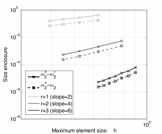
Figure 1. Log-log graph associated to $\Omega_{\mathrm{c}}$ and $\omega_{2}=\sqrt{3}$. Vertical axis: enclosure width. Horizontal axis: maximum element size $h$. Here we have chosen Lagrange elements of order $r=1,2,3$ on a sequence of unstructured meshes. Here we have chosen $t=\frac{\sqrt{2}+\sqrt{3}}{2}$ the upper bounds and $t=\frac{\sqrt{3}+\sqrt{5}}{2}$ for the lower bounds.

Let $\Omega=\Omega_{\mathrm{c}}=(0,\pi)^{3}\subset\mathbb{R}^{3}$. The non-zero eigenvalues are

$$\omega=\pm\sqrt{l^{2}+m^{2}+n^{2}}$$

and the corresponding eigenfunctions are

$${\boldsymbol{E}}(x,y,z)=\begin{pmatrix}\alpha_{1}\cos(lx)\sin(my)\sin(nz)\\ \alpha_{2}\sin(lx)\cos(my)\sin(nz)\\ \alpha_{3}\sin(lx)\sin(my)\cos(nz)\end{pmatrix}\qquad\forall\underline{\alpha}:=\begin{pmatrix}\alpha_{1}\\ \alpha_{2}\\ \alpha_{3}\end{pmatrix}\mbox{ s.t. }\underline{\alpha}\cdot\begin{pmatrix}l\\ m\\ n\end{pmatrix}=0.$$

Here $\{l,m,n\}\subset\mathbb{N}\cup\{0\}$ and not two indices are allowed to vanish simultaneously. The vector $\underline{\alpha}$ determines the multiplicity of the eigenvalue for a given triplet $(l,m,n)$. That is, for example, $\omega_{1}=\sqrt{2}$ (the first positive eigenvalue) has multiplicity 3 corresponding to indices $\{(1,1,0),(0,1,1),(1,0,1)\}$ each one of them contributing to one of the dimensions of the eigenspace. However, $\omega_{2}=\sqrt{3}$ (the second positive eigenvalue) corresponding to index $\{(1,1,1)\}$ has multiplicity 2 determined by $\underline{\alpha}$ on a plane.

In Figure 1 we have depicted the decrease in enclosure width and exact residual,

$$\omega^{+}_{2}-\omega^{-}_{2}\qquad\text{and}\qquad\omega^{+}_{2}-\omega_{2},$$

for the computed bounds of the eigenvalue $\omega_{2}=\sqrt{3}$ by means of Lagrange elements of order $r=1,2,3$. In this experiment we have chosen a sequence of unstructured tetrahedral mesh. The values for the slopes of the straight lines indicates that the enclosures obey the estimate of the form

(43) $$|\omega^{\pm}-\omega|\leq ch^{2r},$$

which is indeed the optimal convergence rate.

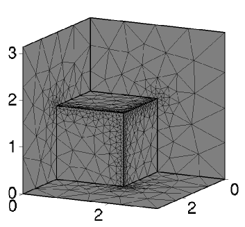
$k$	$(\omega_{k})_{-}^{+}$
$1$	$1.1^{46}_{25}$
$2$	$1.54^{41}_{16}$
$3$	$1.54^{41}_{18}$
$4$	$2.0^{82}_{64}$
$5$	$2.0^{82}_{78}$
$6$	$2.0^{82}_{78}$
$7$	$2.2^{35}_{13}$
$8$	$2.2^{35}_{14}$
$9$	$2.32^{67}_{58}$
$10$	$2.33^{23}_{09}$
$11$	$2.33^{24}_{10}$
$12$	$2.^{40}_{36}$
$13$	$2.^{60}_{59}$
$14$	$2.^{60}_{59}$
$15$	$2.60^{56}_{09}$

Figure 2. Spectral enclosures for the spectrum lying on the interval $(0,2\sqrt{2})$ for the Fichera domain $\Omega_{\mathrm{F}}$. Here we have fixed $t=0.2$ to compute the upper bounds and $t=2.8$ to compute the lower bounds. We considered mesh refined at the re-entrant edges as shown on the left. The number of DOF=208680.

5.2. Benchmark eigenvalue bounds for the Fichera domain

In this next experiment we consider the region $\Omega=\Omega_{\mathrm{F}}=(0,\pi)^{3}\setminus[0,\pi/2]^{3}$. Some of the eigenvalues can be obtained by domain decomposition and the corresponding eigenfunctions are regular. For example, eigenfunctions on the cube of side $\pi/2$ can be assembled in the obvious fashion, in order to build eigenfunctions on $\Omega_{\mathrm{F}}$. Therefore the set $\{\pm 2\sqrt{l^{2}+m^{2}+n^{2}}\}$ where not two indices vanish simultaneously certainly lies inside $\sigma(\mathcal{M})$. The first eigenvalue in this set is $2\sqrt{2}$.

We conjecture that there are exactly $15$ eigenvalues in the interval $(0,2\sqrt{2})$. Furthermore, we conjecture that the multiplicity counting of the spectrum in this interval is

$$1,\,2,\,3,\,2,\,1,\,2,\,1,\,3.$$

The table on the right of Figure 2 shows a numerical estimation of these eigenvalues. We have considered a mesh refined along the re-entrant edges as shown on the left side of this figure.

The slight numerical discrepancy shown in the table for the seemingly multiple eigenvalues appears to be a consequence of the fact that the meshes employed are not entirely symmetric with respect to permutation of the spacial coordinates.

Appendix A A Comsol v4.3 LiveLink code

%     Comsol V4.3 LiveLink code for computing
%   fundamental frequencies on a resonant cavity
%      with perfect conductivity conditions
% the test geometry below is the Fichera domain.
%
%      Gabriel Barrenechea, Lyonell Boulton
%              and Nabile Boussaid
%                                       November 2012

% INITIALIZATION OF THE MODEL FROM SCRATCHES

model = ModelUtil.create(’Model’);
geom1=model.geom.create(’geom1’, 3);
mesh1=model.mesh.create(’mesh1’, ’geom1’);
w=model.physics.create(’w’, ’WeakFormPDE’, ’geom1’,
              {’E1’,’E2’, ’E3’, ’H1’, ’H2’, ’H3’});

% CREATING THE GEOMETRY - IN THIS CASE THE FICHERA DOMAIN

hex1=geom1.feature.create(’hex1’, ’Hexahedron’);
hex1.set(’p’,{’0’ ’0’ ’0’ ’0’ ’pi’ ’pi’ ’pi’ ’pi’;
              ’0’ ’0’ ’pi’ ’pi’ ’0’ ’0’ ’pi’ ’pi’;
              ’0’ ’pi’ ’pi’ ’0’ ’0’ ’pi’ ’pi’ ’0’});
hex2=geom1.feature.create(’hex2’, ’Hexahedron’);
hex2.set(’p’,{’0’ ’0’ ’0’ ’0’ ’pi/2’ ’pi/2’ ’pi/2’ ’pi/2’;
              ’0’ ’0’ ’pi/2’ ’pi/2’ ’0’ ’0’ ’pi/2’ ’pi/2’;
              ’0’ ’pi/2’ ’pi/2’ ’0’ ’0’ ’pi/2’ ’pi/2’ ’0’});
dif1 = geom1.feature.create(’dif1’, ’Difference’);
dif1.selection(’input’).set({’hex1’});
dif1.selection(’input2’).set({’hex2’});
geom1.run;

%CREATING THE GEOMETRY
model.mesh(’mesh1’).automatic(false);
model.mesh(’mesh1’).feature(’size’).set(’custom’, ’on’);
model.mesh(’mesh1’).feature(’size’).set(’hmax’, ’.8’);
mesh1.run;

% PARAMETER t WHERE TO LOOK FOR EIGENVALUES
parat=2.2;

% WHETHER TO LOOK FOR THE EIGENVALUES TO THE LEFT (-) OR
% RIGHT (+) AND WHERE ABOUT
shi=-.3;
model.param.set(’tt’, num2str(parat));
searchtau=shi;

% FINITE ELEMENTS TO USE AND ORDER
w.prop(’ShapeProperty’).set(’shapeFunctionType’, ’shlag’);
w.prop(’ShapeProperty’).set(’order’, 3);

% PHYSICS
w.feature(’wfeq1’).set(’weak’,1 ,’(H3y-H2z)*(H3y_test-H2z_test)-
i*2*tt*(H3y-H2z)*E1_test+tt^2*E1*E1_test+(i*(H3y-H2z)-tt*E1)*E1t_test’);
w.feature(’wfeq1’).set(’weak’,2 ,’(H1z-H3x)*(H1z_test-H3x_test)-
i*2*tt*(H1z-H3x)*E2_test+tt^2*E2*E2_test+(i*(H1z-H3x)-tt*E2)*E2t_test’);
w.feature(’wfeq1’).set(’weak’,3 ,’(H2x-H1y)*(H2x_test-H1y_test)-
i*2*tt*(H2x-H1y)*E3_test+tt^2*E3*E3_test+(i*(H2x-H1y)-tt*E3)*E3t_test’);
w.feature(’wfeq1’).set(’weak’,4 ,’(E3y-E2z)*(E3y_test-E2z_test)+
i*2*tt*(E3y-E2z)*H1_test+tt^2*H1*H1_test+((-i)*(E3y-E2z)-tt*H1)*H1t_test’);
w.feature(’wfeq1’).set(’weak’,5 ,’(E1z-E3x)*(E1z_test-E3x_test)+
i*2*tt*(E1z-E3x)*H2_test+tt^2*H2*H2_test+((-i)*(E1z-E3x)-tt*H2)*H2t_test’);
w.feature(’wfeq1’).set(’weak’,6 ,’(E2x-E1y)*(E2x_test-E1y_test)+
i*2*tt*(E2x-E1y)*H3_test+tt^2*H3*H3_test+((-i)*(E2x-E1y)-tt*H3)*H3t_test’);

% BOUNDARY CONDITIONS
cons1=model.physics(’w’).feature.create(’cons1’, ’Constraint’);
cons1.set(’R’, 2, ’E2’);
cons1.set(’R’, 3, ’E3’);
cons1.selection.set([1 8 9]);
cons2=model.physics(’w’).feature.create(’cons2’, ’Constraint’);
cons2.set(’R’, 1, ’E1’);
cons2.set(’R’, 3, ’E3’);
cons2.selection.set([2 5 7]);
cons3=model.physics(’w’).feature.create(’cons3’, ’Constraint’);
cons3.set(’R’, 1, ’E1’);
cons3.set(’R’, 2, ’E2’);
cons3.selection.set([3 4 6]);

% HOW MANY EIGENVALUES TO LOOK FOR AROUND t
neval=3;

% SOLVING THE MODEL
std1=model.study.create(’std1’);
model.study(’std1’).feature.create(’eigv’, ’Eigenvalue’);
model.study(’std1’).feature(’eigv’).set(’shift’, num2str(searchtau));
model.study(’std1’).feature(’eigv’).set(’neigs’, neval);
std1.run;

% STORING SOLUTION FOR POST PROCESSING
[SZ,NDOFS,DATA,NAME,TYPE]= mphgetp(model,’solname’,’sol1’);



% DISPLAYING SOLUTION
for inde=1:neval,
tauinv=(real(DATA(inde)));
bd=parat+tauinv;
if tauinv<0, disp([’lower= ’,num2str(bd,10)]);
else disp([’upper= ’,num2str(bd,10)]);
end
disp([’DOF= ’,num2str(NDOFS)])
end

References

- [1] C. Amrouche, C. Bernardi, M. Dauge, and V. Girault, Vector potentials in three-dimensional non-smooth domains, Math. Methods Appl. Sci., 21 (1998), pp. 823–864.
- [2] D. Arnold, R. Falk, and R. Winther, Finite element exterior calculus: from hodge theory to numerical stability, Bulletin of the American Mathematical Society, 47 (2010), pp. 281–354.
- [3] H. Behnke, Lower and upper bounds for sloshing frequencies, Inequalities and Applications, (2009), pp. 13–22.
- [4] H. Behnke and U. Mertins, Bounds for eigenvalues with the use of finite elements, Perspectives on Enclosure Methods, (2001), p. 119.
- [5] P. Bernhard and A. Rapaport, On a theorem of Danskin with an application to a theorem of von Neumann-Sion, Nonlinear Anal., 24 (1995), pp. 1163–1181.
- [6] M. Birman and M. Solomyak, The self-adjoint Maxwell operator in arbitrary domains, Leningrad Math. J, 1 (1990), pp. 99–115.
- [7] D. Boffi, Finite element approximation of eigenvalue problems, Acta Numer., 19 (2010), pp. 1–120.
- [8] D. Boffi, P. Fernandes, L. Gastaldi, and I. Perugia, Computational models of electromagnetic resonators: analysis of edge element approximation, SIAM J. Numer. Anal., 36 (1999), pp. 1264–1290 (electronic).
- [9] A. Bonito and J.-L. Guermond, Approximation of the eigenvalue problem for the time harmonic Maxwell system by continuous Lagrange finite elements, Math. Comp., 80 (2011), pp. 1887–1910.
- [10] L. Boulton and M. Strauss, Eigenvalue enclosures for the MHD operator, BIT Numerical Mathematics, (2012).
- [11] J. H. Bramble, T. V. Kolev, and J. E. Pasciak, The approximation of the Maxwell eigenvalue problem using a least-squares method, Math. Comp., 74 (2005), pp. 1575–1598 (electronic).
- [12] A. Buffa, P. Ciarlet, and E. Jamelot, Solving electromagnetic eigenvalue problems in polyhedral domains, Numer. Math., 113 (2009), pp. 497–518.
- [13] F. Chatelin, Spectral Approximation of Linear Operators, Academic Press, New York, 1983.
- [14] P. Ciarlet, The finite element method for elliptic problems, North-Holland, Amsterdam, 1978.
- [15] E. B. Davies, Spectral enclosures and complex resonances for general self-adjoint operators, LMS J. Comput. Math, 1 (1998), pp. 42–74.
- [16] , A hierarchical method for obtaining eigenvalue enclosures, Math. Comp., 69 (2000), pp. 1435–1455.
- [17] E. B. Davies and M. Plum, Spectral pollution, IMA J. Numer. Anal., 24 (2004), pp. 417–438.
- [18] A. Ern and J.-L. Guermond, Theory and practice of finite elements, vol. 159 of Applied Mathematical Sciences, Springer-Verlag, New York, 2004.
- [19] V. Girault and P.-A. Raviart, Finite element methods for Navier-Stokes equations, vol. 5 of Springer Series in Computational Mathematics, Springer-Verlag, Berlin, 1986. Theory and algorithms.
- [20] F. Goerisch and J. Albrecht, The convergence of a new method for calculating lower bounds to eigenvalues, in Equadiff 6 (Brno, 1985), vol. 1192 of Lecture Notes in Math., Springer, Berlin, 1986, pp. 303–308.
- [21] G. Strang and G. Fix, An Analysis of the Finite Element Method, Prentice Hall, London, 1973.
- [22] H. F. Weinberger, Variational Methos for Eigenvalue Approximation, Society for Industrial and Applied Mathematics, Philadelphia, 1974.
- [23] S. Zimmermann and U. Mertins, Variational bounds to eigenvalues of self-adjoint eigenvalue problems with arbitrary spectrum, Z. Anal. Anwendungen, 14 (1995), pp. 327–345.