A Toroidal Magnetised Iron Neutrino Detector (MIND) for a Neutrino Factory

Abstract

A neutrino factory has unparalleled physics reach for the discovery and measurement of CP violation in the neutrino sector. A far detector for a neutrino factory must have good charge identification with excellent background rejection and a large mass. An elegant solution is to construct a magnetized iron neutrino detector (MIND) along the lines of MINOS, where iron plates provide a toroidal magnetic field and scintillator planes provide 3D space points. In this report, the current status of a simulation of a toroidal MIND for a neutrino factory is discussed in light of the recent measurements of large $\theta_{13}$. The response and performance using the 10 GeV neutrino factory configuration are presented. It is shown that this setup has equivalent $\delta_{CP}$ reach to a MIND with a dipole field and is sensitive to the discovery of CP violation over 85% of the values of $\delta_{CP}$.

I Introduction

The neutrino factory is a new type of accelerator facility in which a neutrino beam is created from the decay of muons in flight in a storage ring. This facility can be used to study neutrino oscillations in a variety of oscillation channels Geer (1998) and can be used to determine the neutrino mass hierarchy, whether the mass squared difference between neutrino mass eigenstates $\Delta m^{2}_{13}$ is positive or negative (inverted or normal mass hierarchy), and CP violation in the neutrino sector. The $\nu_{e}\rightarrow\nu_{\mu}$ oscillation De Rújula et al. (1999), identified through the so-called “golden channel” in which the charged current interactions of the $\nu_{\mu}$ produce muons of the opposite charge to those stored in the storage ring (wrong-sign muons) Cervera et al. (2000), is the most promising channel to explore CP violation at a neutrino factory. The physics capabilities and the design of the neutrino factory is carried out as part of the International Design Study for a Neutrino Factory (IDS-NF) IDS , partially funded through the EUROnu project EUR .

In this paper we will describe the requirements and design of a neutrino factory far detector and the analysis carried out to extract the wrong-sign muon neutrino oscillation signal. The far detector at a neutrino factory Choubey et al. (2011) requires excellent reconstruction and charge detection efficiency. These capabilities are best encompassed using a large magnetized iron neutrino detector (MIND). For the discussion below, a MIND design with a toroidal magnetic field, based on experience from the MINOS far detector Michael et al. (2008) is described with detailed simulations.

With the measurement of large $\theta_{13}$ Abe et al. (2011); An et al. (2012); Ahn et al. (2012); Abe et al. (2012); Adamson et al. (2011a) the physics goals of the neutrino factory are focused on the measurement of CP violation and the mass hierarchy in neutrino oscillations. This requires re-optimization of the neutrino factory baseline and re-evaluating the detector for this physics goal. The new experimental setup consists of a single 2000 km baseline from a muon storage ring wherein both $\mu^{+}$ and $\mu^{-}$ decay at energies of 10 GeV to a single 100 kTon detector with a toroidal magnetic field. The analysis described here improves and simplifies a previous analysis based on a 100 kton detector with a dipole magnetic field Bayes et al. (2012).

The neutrino beam from a neutrino factory contains both $\nu_{\mu}(\bar{\nu}_{\mu})$ and $\bar{\nu}_{e}(\nu_{e})$ resulting from the decay of $\mu^{-}(\mu^{+})$ in a storage ring. As such, there are a number of possible oscillation channels, summarized in Table 1. The MIND is optimized to exploit the golden channel oscillation as this has an easily identified signal; a muon with a sign opposite to that in the muon storage ring. With the exception of the silver channel oscillation, which re-enforces the golden channel signal, other oscillation channels are treated as background. The event selection required to produce the best signal and background rates for the measurement of CP violation is the focus of ongoing optimization.

This paper describes the detector design (Section II) before discussing the simulation (Section III) and event reconstruction (Section IV). Event selection is given in Section V and the resulting efficiency and background rates are presented in Section VI. Finally, the sensitivity and precision of the detector to CP violation is presented in Section VII.

Table 1: List of oscillations expected at a neutrino factory.

	Store $\mu^{+}$	Store $\mu^{-}$
Golden Channel	$\nu_{e}\to\nu_{\mu}$	$\bar{\nu}_{e}\to\bar{\nu}_{\mu}$
$\nu_{e}$ Disappearance Channel	$\nu_{e}\to\nu_{e}$	$\bar{\nu}_{e}\to\bar{\nu}_{e}$
Silver Channel	$\nu_{e}\to\nu_{\tau}$	$\bar{\nu}_{e}\to\bar{\nu}_{\tau}$
Platinum Channel	$\bar{\nu}_{\mu}\to\bar{\nu}_{e}$	$\nu_{\mu}\to\nu_{e}$
$\nu_{\mu}$ Disappearance Channel	$\bar{\nu}_{\mu}\to\bar{\nu}_{\mu}$	$\nu_{\mu}\to\nu_{\mu}$
Dominant Oscillation	$\bar{\nu}_{\mu}\to\bar{\nu}_{\tau}$	$\nu_{\mu}\to\nu_{\tau}$

II Detector Design

The MIND is an iron-scintillator calorimeter with an octagonal cross section 14 m high and 14 m in width (Fig. 1). Modules of 3 cm thick iron plates and a 2 cm thick lattice of scintillating bars compose the 100 kTon bulk of the detector. The iron planes provide the structural strength for the calorimeter as well as the magnetic field necessary for charge discrimination. Due to practical constraints, the iron planes are to be constructed of strips of steel 1.5 cm thick and 2 m wide. By arranging these strips in a lattice configuration, the resulting structure possesses the necessary rigidity and tensile strength to support its own weight by two “ears” projecting from the sides of the plate, with distortions in the plate dimensions of less than 2 mm.

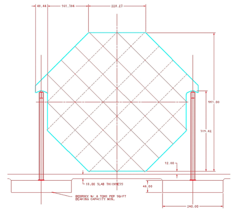
(a) Engineering drawing of the MIND plate

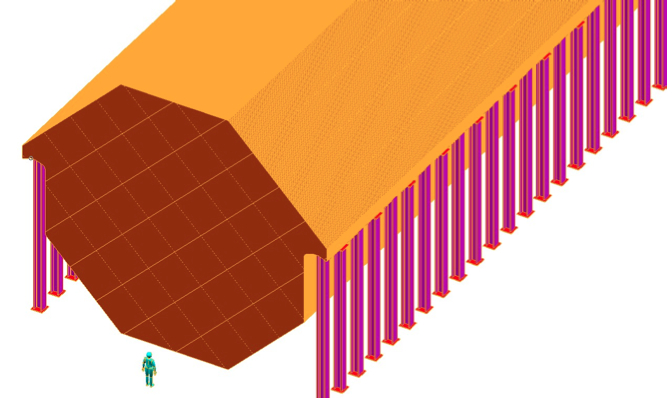
(b) Orthographic view of MIND

Figure 1: Schematic representations of the MIND for a neutrino factory.

To induce the 1 Tesla magnetic field in the iron plate, a current of 100 kA through the centre of the detector is required. This current is to be carried by a super-conducting transmission line (STL), which consists of copper and copper/NbTi alloy braids contained by a cryogenic jacket, 7 cm in diameter Ambrosio et al. (2001); Foster, G.W. and Kashikhin, V.S. and Malamud, E. and Mazur, P. and Oleck, A. and Piekarz, H. and Fuerst, J. and Rabehl, R. and Schlabach, P. and Volk, J. (2000). The STL runs through a 10 cm bore along the central axis of the detector. A detailed diagram of the STL is shown in Fig. 2. A map of the magnetic field in the iron has been generated using a finite element model of the detector plate. The simulated field map is shown in Fig. 3.

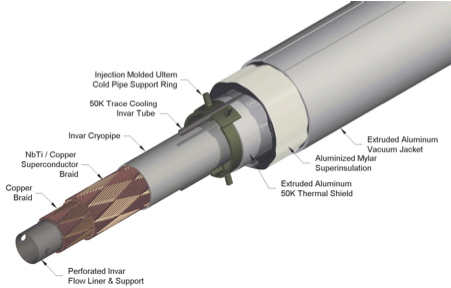
Figure 2: The super-conducting transmission line, proposed as a current source for MIND

Figure 3: The magnetic field in iron simulated from the finite element studies of the MIND plate assuming an STL current of 100 kA

The detection of neutrino interactions is accomplished through the use of scintillating bars arranged in a lattice to define a 3D space point for the energy deposition of a passing particle. Assuming a coordinate system for the detector such that the neutrino beam defines the $z$-axis, perpendicular to the detector face, the scintillator bars are arranged in a layer to measure the position of an event hit along the $x$-axis and a layer to measure a hit position along the $y$-axis. Each scintillator bar is rectangular with a 1 cm$\times$3.5 cm cross-section and spans the width of the detector. A wavelength shifting fibre 1 mm thick runs down the centre of the scintillating bar and is coupled at each end of the bar to a silicon photomultiplier.

III Simulation

Neutrino interactions in the MIND simulation are generated using the GENIE framework Andreopoulos et al. (2010). This framework reproduces deep inelastic scattering (DIS), quasi-elastic scattering (QES), single pion production, resonant pion production, coherent pion production, and neutrino-electron elastic scattering processes. Previous simulation studies for MIND Cervera et al. (2010) have been produced using LEPTO Ingelman et al. (1997) and NUANCE Casper (2002). These packages are incomplete descriptions of the neutrino interactions as they do not include such phenomena as re-interaction within participant nuclei; an important feature in high Z targets such as iron.

The detector geometry was constructed using the GEANT4 framework Allison et al. (2006). The geometry was defined with some flexibility in the detector dimensions, including the transverse and longitudinal lengths as well as the thickness of the iron and scintillator planes to allow for optimization studies. The magnetic field, although basically toroidal, is applied using a field map. Products of the neutrino interaction events generated by GENIE are propagated through the detector materials using the QGSP_BERT physics list provided by GEANT4.

IV Reconstruction

Following simulation, the events are digitized in a very simple way. The position and energy deposition for a hit in a given scintillator plane are clustered in a 3.5 cm$\times$3.5 cm unit, called a voxel, which is defined by the expected positions of the scintillator bars in the transverse plane. The energy deposition is attenuated over the distance of the hit from the edge of the detector assuming an attenuation length of 5 m. The digitized hits are passed to a reconstruction module.

The purpose of the reconstruction is to identify and fit potential muon tracks resulting from charge current neutrino interactions. The reconstruction uses algorithms provided by the RecPack toolkit Cervera-Villanueva et al. (2004). The majority of tracks are identified from the event using a Kalman filtering algorithm. First a prospective track is identified by looking for the longest set of planes with a single digitized hit. A guess for an initial angle and momentum is generated from this information and used for an initial fit. Additional hits are then filtered into the track by looking for hits that produce the smallest local $\chi^{2}$ value in planes with multiple hit occupancies. The subset of events that do not have a set of single occupancy planes are subjected to a cellular automaton algorithm Abt et al. (2002) for the identification of tracks within events where the muon track is not separated from the hadron activity. In either case the longest track is selected as the muon trajectory passed to the fitting algorithm.

The identified muon tracks are subject to a Kalman fitting process to determine their momentum and charge. The Kalman fitter uses a model to predict the position from one hit to the next in a sequence correcting for random noise, such as from multiple scattering, and allowing for processes such as energy loss — which is now included as a function of momentum. An initial seed for the fit is determined from the geometry of the muon track using the range of the muon track to supply the momentum Groom et al. (2001) and the relative positions of the beginning and end of the track in the bending plane to determine the charge. This seed is passed to the fitting algorithm where the track parameters are further refined. A successfully reconstructed track survives the Kalman fitting process six times; twice during the track identification stage where the track is fitted and filtered and four more times during the fitting stage assuming different fitting seeds. These algorithms are based on previous work Cervera et al. (2010); Bayes et al. (2012), but adapted to the new toroidal magnetic field configuration. The momentum resolution resulting from this fit is shown in Fig. 4. The behaviour of the resolution on the inverse of the momentum ($1/p$) is parametrized as follows;

$$\frac{\sigma_{1/p}}{1/p}=0.24-\frac{0.061}{p(GeV)}+0.11p.$$ (1)

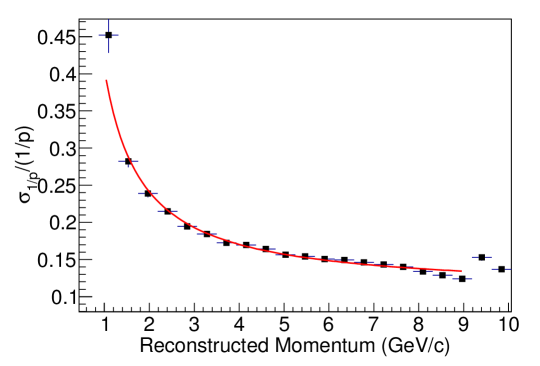
Figure 4: Momentum resolution from the muon track reconstruction. The parametrization of the resolution measured from the simulation is shown with the red solid line.

The neutrino energy is currently reconstructed using the combination of the reconstructed muon momentum and the smeared true hadron energy, $E_{had}$. This smearing assumes an energy resolution $\delta E_{had}$ measured from the MINOS CalDet test beam Michael et al. (2008);

$$\frac{\delta E_{had}}{E_{had}}=\frac{0.55}{\sqrt{E_{had}}}\oplus 0.03.$$ (2)

Since Ref. Michael et al. (2008) does not provide the angular resolution, this was taken from the measurements at the Monolith test beam Bari et al. (2003);

$$\delta\theta_{had}=\frac{10.4}{\sqrt{E_{had}}}\oplus\frac{10.1}{E_{had}}.$$ (3)

Current work to explicitly identify and reconstruct the hadron showers will remove the necessity of this smearing process for the generation of a reconstructed energy. In the case of quasi-elastic (QES) events, the neutrino energy is calculated from the expression

$$E_{\nu}=\frac{m_{N}E_{\mu}+\frac{1}{2}(m^{2}_{N^{\prime}}-m^{2}_{\mu}-m^{2}_{N})}{m_{N}-E_{\mu}+|p_{\mu}|\cos\vartheta}$$ (4)

where $\vartheta$ is the angle between the muon momentum vector and the beam direction, $m_{N}$ is the mass of the initial state nucleon and $m_{N^{\prime}}$ is the mass of the final state nucleon in the processes $\nu_{\mu}+n\to\mu^{-}+p$ and $\bar{\nu}_{\mu}+p\to\mu^{+}+n$.

V Analysis

Successfully reconstructed events are subjected to a series of cuts to isolate the wrong sign muons resulting from $\nu_{e}\to\nu_{\mu}$ oscillations from backgrounds that are similar to neutral current events. All cuts used in the analysis are summarized in Table 2 and are similar to those from a previous analysis Bayes et al. (2012). The first cut ensures that the event is successfully reconstructed by the Kalman filter. The second cut removes events for which the first scintillator hit appears less than 1.5 m from the end of the detector. Tracks reconstructed with momenta greater than 16 GeV are removed to reduce biases from non-physical reconstructed neutrino energies. A cut is also applied requiring that 60% of the candidate hits of the track are used in the final fit, to avoid tracks with hard scattering events or other sources of noise.

Event Cut	Description
Successful Reconstruction	Failed Kalman reconstruction of event removed
Fiducial	First hit of event is more than 1.5 m from end of detector
Maximum Momentum	Muon momentum less than 1.6$\times E_{\mu}$
Fitted Proportion	60% of track nodes used in final fit.
Track Quality	$\log(P(\sigma_{q/p}/(q/p)|CC)/P(\sigma_{q/p}/(q/p)|NC))>-0.5$
CC Selection	$\log(P(N_{hit}|CC)/P(N_{hit}|NC))>1.0$
Kinematic	$Q_{t}>0.15GeV$

Table 2: Description of cuts used in the selection of good events from the simulation

Two cuts deserve special attention as they provide most of the discriminating power between the Golden channel oscillation signal and background events. Both use a log-likelihood approach to select between charge current and neutral current interactions. The likelihood derived from the probability of the normalized uncertainty in $q/p$ (the charge over the momentum from the fit to each track) for charge current events $P(\sigma_{q/p}/(q/p)|CC)$ with respect to the same for neutral current events $P(\sigma_{q/p}/(q/p)|NC)$ is

$$\mathcal{L}_{q/p}=\log\left(\frac{P(\sigma_{q/p}/(q/p)|CC)}{P(\sigma_{q/p}/(q/p)|NC)}\right),$$ (5)

which provides good separation between signal and background when $\mathcal{L}_{q/p}>-0.5$. This cut was chosen through consideration of the distributions of $\mathcal{L}_{q/p}$ for the simulated neutrino species as shown in Fig. 5.

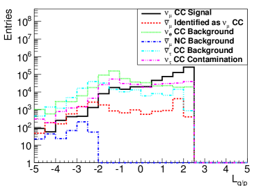
(a) Stored $\mu^{+}$ experiment

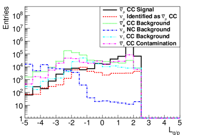
(b) Stored $\mu^{-}$ experiment

Figure 5: Distribution of $\mathcal{L}_{q/p}$ for simulated neutrino species.

A stronger charge current selection is defined by the number of hits in the track. Muon tracks travel much further within the detector, so they produce many more hits than electron or hadron showers, which are known to range out quickly. To make this cut without bias a likelihood ratio was defined as the probability of a track appearing with a given number of hits assuming a charge current event $P(N_{hit}|CC)$ to the same probability assuming a neutral current event $P(N_{hit}|CC)$;

$$\mathcal{L}_{CC}=\log\left(\frac{P(N_{hit}|CC)}{P(N_{hit}|NC)}\right).$$ (6)

The best separation between signal and background occurs when events with $\mathcal{L}_{CC}>1.0$ are kept. The $\mathcal{L}_{CC}$ distributions for the simulated neutrino species are shown in Fig. 6.

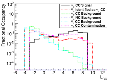
(a) Stored $\mu^{+}$ experiment

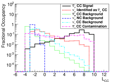
(b) Stored $\mu^{-}$ experiment

Figure 6: Distribution of $\mathcal{L}_{CC}$ for simulated neutrino species.

A further cut is applied on the kinematic variables of the event. By placing a cut on the separation of the muon direction and the direction of hadronization, some further separation between signal events and $\nu_{e}$ CC events can be achieved. For a 10 GeV neutrino factory a cut on the separation variable $Q_{t}=E_{\nu}\sin\theta>0.15$ GeV, where $\theta$ is the angle between the muon candidate and the hadronic-jet vector, was found to provide this. The effect of the cuts on the event samples is summarized in Fig. 7 and 8.

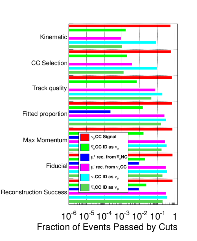
(a) Stored $\mu^{+}$ experiment

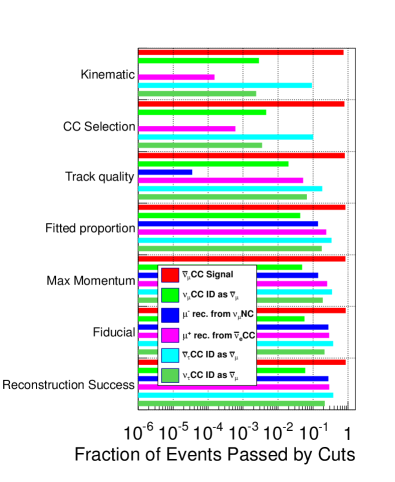
(b) Stored $\mu^{-}$ experiment

Figure 7: Effect of the cuts on the detection of signal and background events assuming a magnetic field that focusses positively charged particles.

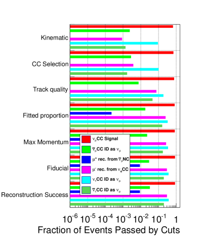
(a) Stored $\mu^{+}$ experiment

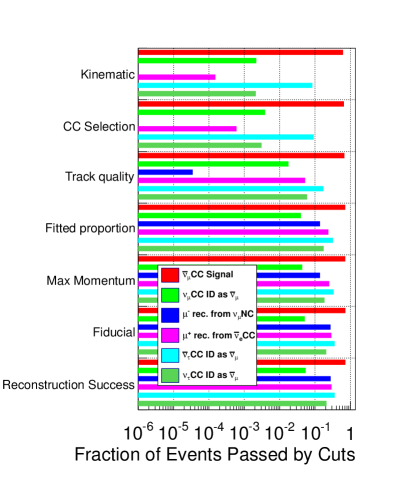
(b) Stored $\mu^{-}$ experiment

Figure 8: Effect of the cuts on the detection of signal and background events assuming a magnetic field that focusses negatively charged particles.

A multi-variate analysis for the identification of $\nu_{\mu}(\bar{\nu}_{\mu})$ CC events is also under consideration. Based on the experience of the MINOS experiment Adamson et al. (2011b) it is believed that an analysis, such as a $k$-nearest neighbour approach, using multiple correlated variables can produce a better discrimination between signal and background events. A set of variables that includes the mean energy deposition along the muon track, the variation of the energy deposition, and the total number of track hits is under consideration for this purpose. This is work in progress.

VI Detector Efficiencies and Response

The efficiencies and background suppression for MIND in the muon neutrino appearance channel is shown in Fig. 9 and Fig. 10. Four cases are considered in these figures depending on the binary state of the storage ring and the detector; a $\mu^{-}(\mu^{+})$ is contained in the storage ring resulting in a $\bar{\nu}_{\mu}(\nu_{\mu})$ signal, and the magnetic field of MIND focusses $\mu^{+}(\mu^{-})$. A neutrino factory stores both $\mu^{-}$ and $\mu^{+}$ in the ring so that pulses of neutrinos associated with decays of each species can be identified based on their correlated time structure. However the magnetic field direction must be chosen a priori based on an understanding of the detector response and resulting sensitivity to the CP violation.

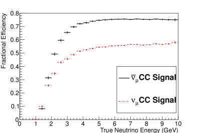
(a) Signal detection efficiency in a $\mu^{+}$ focussing field

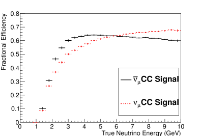
(b) Signal detection efficiency in a $\mu^{-}$ focussing field

Figure 9: Efficiency for the detection of $\nu_{\mu}$ and $\bar{\nu}_{\mu}$ charge current detection assuming the two different magnetic field configurations.

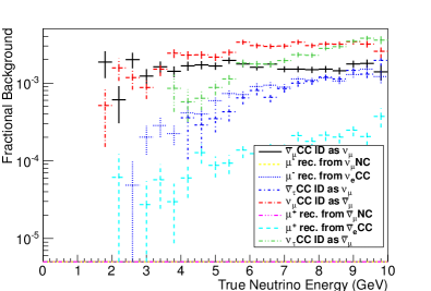
(a) Background rates in a $\mu^{+}$ focussing field

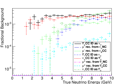
(b) Background rates in a $\mu^{-}$ focussing field

Figure 10: Background rates for $\nu_{\mu}$ and $\bar{\nu}_{\mu}$ charge current detection assuming the two different magnetic field configurations.

VII Sensitivities

The analysis of the simulation is used to generate “migration matrices” that relate the true neutrino energy to the reconstructed neutrino energy and contain all of the information regarding the reconstruction efficiency, energy response, and resolution. These migration matrices ($M_{ij}$) are used to convert a set of neutrino counts ($\nu(E_{j})$) calculated using a long baseline simulation into expected counts in a detector as a function of energy ($n(E_{i})$) i.e. $n(E_{i})=M_{ij}\nu(E_{j})$. The Neutrino tool suite (NuTS), developed for the studies presented in Burguet-Castell et al. (2001, 2002, 2005), is a framework that generates the event rates $\nu(E_{j})$ from the appropriate fluxes and is used to extract the neutrino oscillation probabilities for all channels.

The pseudo-experimental data is extracted from a combination of the signal and background species,

$$n^{data}_{i}=M^{sig}_{ij}\nu^{sig}(E_{j})+\sum_{k}M^{bkg,k}_{ij}\nu^{bkg,k}(E_{j}),$$ (7)

and compared with an oscillation hypothesis using a $\chi^{2}$ statistic such as

$$\chi^{2} =2\displaystyle\sum_{i=0}^{L}\Bigg{(} AxN_{+,i}(\theta_{13},\delta_{CP})-n^{data}_{+,i}+n^{data}_{+,i}\ln\left(\frac{n^{data}_{+,i}}{AxN_{+,i}(\theta_{13},\delta_{CP})}\right)$$ (8)

$$+AN_{-,i}(\theta_{13},\delta_{CP})-n^{data}_{-,i}+n^{data}_{-,i}\ln\left(\frac{n^{data}_{-,i}}{AN_{-,i}(\theta_{13},\delta_{CP})}\right)$$

$$+\frac{(A-1)^{2}}{\sigma_{A}^{2}}+\frac{(x-1)^{2}}{\sigma_{x}}\Bigg{)}.$$

In this equation $n^{data}_{q,i}$ is the simulated “data” for the energy bin, $i$, assuming a muon signal with a sign $q$, while $N_{q,i}(\theta_{13},\delta_{CP})$ is the predicted content of the corresponding energy bin for the test values of $\theta_{13}$ and $\delta_{CP}$. This fit includes two systematic uncertainties that are assumed to be the leading terms; the error, $\sigma_{x}$, on the ratio $x$ of $\nu$ to $\bar{\nu}$ cross-sections and the error, $\sigma_{A}$, on the total counts in the detector $A$ due to fiducial errors or variation in the neutrino beam. The uncertainty in the cross-section ratio is assumed to be measurable to the 1% level at a neutrino factory, as the near detector sites will take concurrent measurements of both the neutrino and anti-neutrino species Bogomilov et al. (2013). Similarly, measurements at the near detector combined with muon decay rate measurements from instrumentation in the muon decay ring should reduce the uncertainty $\sigma_{A}$ to below 1% Bayes et al. (2012). Conservative upper limits for these errors of 3% and 2.5% respectively are also considered in this study, but the neutrino factory will allow much better control of these systematic uncertainties.

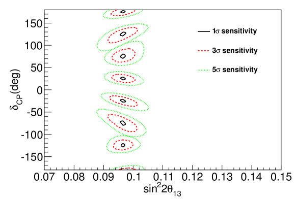
Figure 11: Contours of constant $\chi^{2}$ for a variety of values of $\delta_{CP}$, calculated using Eq. 8. The simulations were generated with the octagonal geometry and a $\mu^{-}$ focussing field. Systematic errors of 1% for both $\sigma_{A}$ and $\sigma_{x}$ are assumed in these fits.

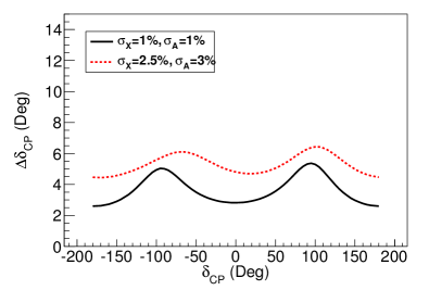
(a) Error assuming a $\mu^{-}$ focussing field.

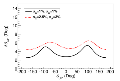
(b) Error assuming a $\mu^{+}$ focussing field.

Figure 12: Uncertainty on $\delta_{CP}$ as a function of $\delta_{CP}$ for the two possible detector field polarities. The black line assumes the 1% systematic uncertainties that are believed will be prevalent at the neutrino factory, while the red line assumes uncertainties inflated by a factor of between 2.5 and 3.

The $\chi^{2}$ contours defined by a series of fits with different values of CP violating phase are shown in Fig. 11. The error of a measurement of the CP violating phase is determined by finding the width of the contour defined by $\chi^{2}=1$ at $\theta_{13}=9.0^{\circ}$. A neutrino factory offers the best prospect to improve the precision of the measurement of $\theta_{13}$. The uncertainty curves for $\delta_{CP}$ derived from simulations using the $\mu^{+}$ and $\mu^{-}$ focusing fields are shown in Fig. 12. Uncertainty curves are identical for the two cases, suggesting that the variation in the momentum response resulting from the change in the detector field properties averages out when the species are added together for the $\chi^{2}$ calculation.

The sensitivity of the neutrino factory to CP violation can be determined by searching for sets of oscillation parameters that satisfy the inequality

$$\max(\chi^{2}(\delta_{CP}=-180^{\circ}),\chi^{2}(\delta_{CP}=0^{\circ}),\chi^{2}(\delta_{13}^{0}=180^{\circ}))-\chi^{2}_{min}\geq n^{2}$$ (9)

where $n$ is the desired significance level for the calculation. The curves showing the sensitivity to CP violation and the corresponding fractional 5$\sigma$ coverage are shown in Fig. 13. A neutrino factory can measure 85% of the possible values of $\delta_{CP}$ within the measured range of $\theta_{13}$ with a 5$\sigma$ significance. No change in these figures results from changing the polarity of the detector field.

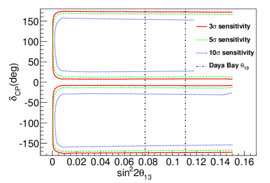
(a) Sensitivity to CP violation, normal hierarchy

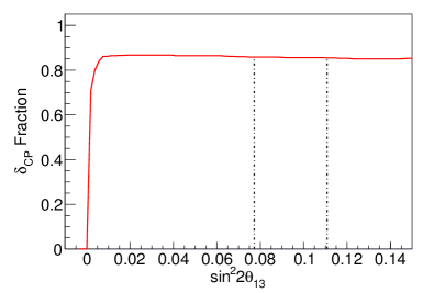
(b) Fractional coverage of 5$\sigma$ sensitivity, normal hierarchy

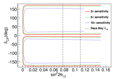
(c) Sensitivity to CP violation,inverted hierarchy

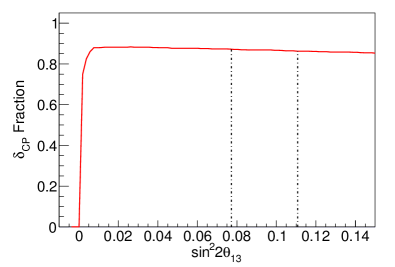
(d) Fractional coverage of 5$\sigma$ sensitivity, inverted hierarchy

Figure 13: Sensitivity of a MIND at a neutrino factory to the discovery of CP violation assuming both a normal and inverted mass hierarchy as noted. The range of $\sin^{2}2\theta_{13}$ measured by Daya Bay is shown with the black dotted line superimposed on the coverage contours and the fractional 5$\sigma$ coverage.

A similar inequality to that shown in Eq. 9 can be defined for the sensitivity to the mass hierarchy. The 5$\sigma$ mass hierarchy discovery potential is achieved for all values of $\theta_{13}$ in which $\sin^{2}2\theta_{13}>10^{-4}$, therefore a neutrino factory will be sensitive to the mass hierarchy for the currently measured value of $\theta_{13}$.

VIII Conclusions

A detailed simulation of a magnetized iron detector with a toroidal field has been produced for neutrino factory studies. This simulation shows that the neutrino factory is capable of discovering CP violation for 85% of the values of the CP violating phase. This result is independent of the mass hierarchy. Given the recent measurements of $\theta_{13}$ by Daya Bay and others, the precision of the measurement is determined to be between $2.5^{\circ}$ and $5.5^{\circ}$ depending on the value of the CP violating phase and assuming leading systematic errors of 1%. Should the sum of the systematics increase to 3.5%, then the largest uncertainty on the measurement of $\delta_{CP}$ is 7^∘. These results assume a measurement based on 5$\times 10^{21}$ muons of both species collected over 10 years.

Further work is in progress to refine these results. Improvement in the reconstruction of multiple tracks for the purpose of identifying hadron showers is in progress and will be implemented soon. Likewise, a multi-variate analysis of the reconstructed simulation is under development. Other studies of the behaviour of MIND will become priorities after the completion of these developments including systematic studies and investigation of the impact of cosmic rays. These studies will come to a conclusion prior to the neutrino factory reference design report due at the end of 2013.

IX Appendix

This appendix summarizes the response matrices of the wrong sign muon signal from $\nu_{\mu}$ and $\bar{\nu}_{\mu}$ appearance and the associated backgrounds in bins of true and reconstructed neutrino energy relevant to an oscillation analysis. Each entry in the table is the survival probability for each species. In all tables, columns represent the true neutrino energy in GeV and rows the reconstructed energy, also in GeV. The overflow bin in reconstructed energy represents all events with a reconstructed energy greater than the known maximum. Migration matrices assuming a negative charge focussing magnetic field and a positive charge focussing magnetic field are shown. The backgrounds generated by $\nu_{\mu}(\bar{\nu}_{\mu})$ NC interactions are consistent with zero at all energies for the 3$\times 10^{6}$ events simulated. Therefore these matrices are not shown.

IX.1 $\nu_{\mu}$ Appearance Matrices, Positive Focussing Detector Field

	0.0-2.0	2.0-2.5	2.5-3.0	3.0-3.5	3.5-4.0	4.0-4.5	4.5-5.0	5.0-5.5	5.5-6.0	6.0-7.0	7.0-8.0	8.0-9.0	9.0-10.0
0.0-2.0	1020	906.9	458.4	213.8	120.2	80.49	52.00	31.51	23.13	12.37	10.26	9.963	6.317
2.0-2.5	421.2	910.5	605.9	318.6	147.8	85.26	56.23	35.77	21.13	10.58	6.357	3.919	3.526
2.5-3.0	202.5	863.7	1010	638.6	335.0	178.2	97.94	61.32	38.83	19.85	10.85	6.708	5.876
3.0-3.5	50.25	482.9	1007	948.1	622.2	345.5	190.9	110.0	70.52	36.37	15.75	9.830	8.080
3.5-4.0	41.38	229.4	687.9	1036	885.6	582.0	342.4	197.4	116.8	58.51	26.94	15.61	12.49
4.0-4.5	11.82	115.3	367.8	792.9	1058	881.1	601.2	366.6	209.7	106.3	40.07	22.52	14.69
4.5-5.0	11.82	30.03	141.9	474.8	859.6	1032	857.5	585.8	358.2	179.7	72.78	30.35	16.45
5.0-5.5	1.478	14.41	50.61	198.1	548.2	870.8	956.9	805.1	557.6	289.8	116.0	52.74	27.03
5.5-6.0	4.434	6.006	21.39	88.10	276.1	598.6	876.9	932.8	789.9	452.0	199.6	82.69	38.34
6.0-7.0	2.956	12.01	22.10	50.95	164.7	459.1	999.4	1505	1735	1409	756.2	346.0	168.1
7.0-8.0	2.956	7.207	14.97	14.29	31.65	87.64	250.5	602.2	1103	1566	1321	759.0	403.8
8.0-9.0	0	3.604	10.69	10.48	16.50	25.15	56.43	148.4	354.9	936.4	1448	1237	815.0
9.0-10.0	1.478	2.402	4.990	6.667	9.091	12.18	16.32	35.94	81.23	347.7	986.0	1355	1208
10.0-11.0	4.434	3.604	9.267	14.29	15.49	19.59	29.42	41.39	57.53	154.4	625.8	1728	2973

Table 3: Golden channel $\nu_{\mu}$ appearance signal efficiency. All values $\times 10^{-4}$.

	0.0-2.0	2.0-2.5	2.5-3.0	3.0-3.5	3.5-4.0	4.0-4.5	4.5-5.0	5.0-5.5	5.5-6.0	6.0-7.0	7.0-8.0	8.0-9.0	9.0-10.0
0.0-2.0	4.903	0	2.659	1.323	2.980	1.165	2.110	1.480	0.8671	1.432	0.8879	0.5123	0.9993
2.0-2.5	0	1.148	1.995	0	0.5960	0	1.407	0.7400	0.2477	0.5834	0.3946	0.1708	0.6246
2.5-3.0	0	0	0.6648	0	0.5960	0.2331	0.1758	0.5920	0.7432	0.5834	0.5920	0.3985	0.7495
3.0-3.5	3.269	0	0	1.765	1.192	1.398	1.231	1.628	0.6194	0.3182	0.4933	0.5123	0.6246
3.5-4.0	0	1.148	0.6648	2.206	0.5960	1.398	0.3517	0.7400	0.8671	0.5834	0.3946	0.3985	1.124
4.0-4.5	0	1.148	1.330	0.8823	0.5960	1.398	1.758	1.184	0.7432	0.4774	0.4933	0.5123	0.6246
4.5-5.0	1.634	1.148	1.330	0.4412	0.8939	1.632	0.3517	1.036	0.3716	1.114	0.3453	0.6262	1.249
5.0-5.5	0	0	1.330	0.4412	1.490	0.9323	0.5275	0.8879	1.239	0.5834	0.2960	1.025	0.2498
5.5-6.0	0	0	1.995	0.8823	0.2980	0.9323	0	1.332	1.486	0.6895	0.8386	0.6831	0.3747
6.0-7.0	0	1.148	0	2.647	0.8939	3.030	2.286	1.628	2.477	1.963	1.381	1.366	1.749
7.0-8.0	0	1.148	1.330	1.323	1.192	1.398	1.758	2.664	1.734	1.856	1.677	1.082	1.624
8.0-9.0	0	0	1.330	0	1.192	0.9323	0.8792	1.776	1.486	1.750	1.529	1.423	1.499
9.0-10.0	1.634	1.148	1.330	0	1.490	1.632	0.5275	1.628	1.363	1.432	1.135	1.537	1.499
10.0-11.0	0	3.445	0	0.8823	1.490	2.098	1.758	2.516	2.849	3.501	4.094	4.554	4.997

Table 4: $\mu^{-}$ background from charge mis-identified $\bar{\nu}_{\mu}$ CC events All values $\times 10^{-4}$.

	0.0-2.0	2.0-2.5	2.5-3.0	3.0-3.5	3.5-4.0	4.0-4.5	4.5-5.0	5.0-5.5	5.5-6.0	6.0-7.0	7.0-8.0	8.0-9.0	9.0-10.0
0.0-2.0	0	0	0.3245	0.2196	0	0.1185	0.0919	0.0775	0.2626	0.1125	0.0528	0.1824	0.2014
2.0-2.5	0	0	0.3245	0.2196	0.3047	0.1185	0.0919	0.0775	0	0.0562	0.0264	0.0608	0
2.5-3.0	0	0	0	0.2196	0	0	0	0.1550	0.0657	0.0562	0.0264	0	0.0671
3.0-3.5	0	0	0.3245	0.2196	0.1524	0	0	0.1550	0.2626	0.1125	0.0792	0.1216	0.0671
3.5-4.0	0	0	0	0	0	0.2370	0.0919	0.1550	0.1970	0.0562	0.2642	0.1216	0.2014
4.0-4.5	0	0	0	0.2196	0.1524	0.1185	0.3675	0.3876	0.5909	0.3375	0.2377	0.0912	0.2686
4.5-5.0	0	0	0	0	0.3047	0.1185	0.1838	0.3101	0.3283	0.4218	0.4226	0.3648	0.3357
5.0-5.5	0	0	0	0.4393	0.1524	0.5924	0.5513	0.6201	0.1313	0.4218	0.3962	0.4864	0.1343
5.5-6.0	0	0	0	0.2196	0.1524	0.5924	0.7351	0.7752	0.6565	0.7593	0.4491	0.3952	0.7386
6.0-7.0	0	0	0	0.6589	0	0.8294	1.195	1.395	0.9191	1.434	1.321	1.337	1.276
7.0-8.0	0	0	0	0.2196	0.4571	0.3555	0.2757	1.008	1.247	1.294	1.559	1.733	1.343
8.0-9.0	0	0	0	0.2196	0.4571	0.4740	0.1838	0.6976	1.247	1.350	1.321	1.520	1.343
9.0-10.0	0	0	0.3245	0	0	0.2370	0.0919	0.4651	0.4596	0.9562	1.506	1.216	1.343
10.0-11.0	0	0	0	0	0	0.2370	0.3675	1.008	0.8535	1.828	2.932	4.104	5.909

Table 5: $\mu^{-}$ background from $\nu_{e}$ CC events. All values $\times 10^{-4}$.

	0.0-2.0	2.0-2.5	2.5-3.0	3.0-3.5	3.5-4.0	4.0-4.5	4.5-5.0	5.0-5.5	5.5-6.0	6.0-7.0	7.0-8.0	8.0-9.0	9.0-10.0
0.0-2.0	0	0	0	128.2	100.00	95.54	72.60	78.94	76.18	70.46	61.40	49.75	41.53
2.0-2.5	0	0	0	0	88.68	75.13	65.80	65.66	62.45	59.56	49.96	41.02	32.78
2.5-3.0	0	0	0	128.2	81.13	87.38	82.06	85.33	81.54	77.24	64.96	57.31	50.62
3.0-3.5	0	0	0	0	60.38	93.91	104.4	98.61	95.94	90.35	77.32	66.57	58.34
3.5-4.0	0	0	0	0	67.92	69.41	85.46	92.46	94.10	93.35	86.64	78.91	64.03
4.0-4.5	0	0	0	0	30.19	52.26	71.09	84.35	85.89	90.75	86.34	78.00	68.37
4.5-5.0	0	0	0	0	18.87	39.20	44.62	65.17	72.50	81.37	85.21	78.30	76.60
5.0-5.5	0	0	0	0	5.660	12.25	23.07	42.79	55.92	72.21	76.45	74.74	70.23
5.5-6.0	0	0	0	0	1.887	9.799	16.64	26.31	39.68	54.64	68.86	71.61	72.95
6.0-7.0	0	0	0	0	1.887	7.349	12.10	22.87	37.67	68.09	102.7	127.1	129.6
7.0-8.0	0	0	0	0	0	2.450	3.781	4.918	11.22	28.03	58.76	88.69	99.62
8.0-9.0	0	0	0	0	0	0.8166	0.7563	2.459	3.851	9.154	26.24	51.84	74.56
9.0-10.0	0	0	0	0	0	0	0.3781	0.7377	1.172	2.712	9.844	22.99	44.42
10.0-11.0	0	0	0	0	1.887	1.633	3.025	2.951	2.512	3.164	6.028	15.56	35.84

Table 6: $\mu^{-}$ reconstructed from $\nu_{\tau}$ CC events. All values $\times 10^{-4}$.

	0.0-2.0	2.0-2.5	2.5-3.0	3.0-3.5	3.5-4.0	4.0-4.5	4.5-5.0	5.0-5.5	5.5-6.0	6.0-7.0	7.0-8.0	8.0-9.0	9.0-10.0
0.0-2.0	0	0	0	0	0	0	0.8818	0.4853	1.102	1.350	1.851	1.887	1.658
2.0-2.5	0	0	0	0	0	0	0	0.7279	0.6295	0.6501	0.9820	1.132	1.357
2.5-3.0	0	0	0	0	0	0	0.4409	0.7279	0.9443	0.8001	1.020	1.283	1.131
3.0-3.5	0	0	0	0	0	0	0	0.4853	0.9443	1.000	0.9820	0.9813	1.507
3.5-4.0	0	0	0	0	0	1.213	0.4409	0.4853	0.7869	0.8501	0.9065	1.547	1.357
4.0-4.5	0	0	0	0	0	0	0	0.7279	0.4721	0.8001	1.095	1.094	1.357
4.5-5.0	0	0	0	0	0	1.213	0	0	0.3148	0.4001	0.5666	0.7926	1.281
5.0-5.5	0	0	0	0	0	0	0	0.7279	0.1574	0.3501	0.5288	0.4152	1.055
5.5-6.0	0	0	0	0	0	0	0.8818	0.2426	0.3148	0.1500	0.5288	0.5661	0.7537
6.0-7.0	0	0	0	0	0	0	0	0	0.1574	0.2500	0.4533	0.9435	1.131
7.0-8.0	0	0	0	0	0	0	0	0	0	0.3501	0.2644	0.6793	1.131
8.0-9.0	0	0	0	0	0	0	0	0	0	0.1500	0.3399	0.1887	0.3015
9.0-10.0	0	0	0	0	0	0	0	0	0	0.1500	0.1889	0.1510	0.2261
10.0-11.0	0	0	0	0	0	0	0	0	0.1574	0.3000	0.1511	0.3774	0.6030

Table 7: $\mu^{-}$ background from $\bar{\nu}_{\tau}$ CC events. All values $\times 10^{-4}$.

IX.2 $\bar{\nu}_{\mu}$ Appearance Matrices, Positive Focussing Detector Field

	0.0-2.0	2.0-2.5	2.5-3.0	3.0-3.5	3.5-4.0	4.0-4.5	4.5-5.0	5.0-5.5	5.5-6.0	6.0-7.0	7.0-8.0	8.0-9.0	9.0-10.0
0.0-2.0	1173	1326	688.8	296.0	156.7	74.59	41.50	23.97	20.69	13.37	11.00	10.08	8.994
2.0-2.5	590.0	1282	865.0	448.7	199.4	99.76	46.78	28.86	20.81	13.10	8.978	5.920	4.622
2.5-3.0	223.9	1263	1373	896.9	449.7	198.8	95.31	54.76	33.32	19.41	12.28	10.47	9.368
3.0-3.5	65.37	666.1	1443	1364	832.6	426.3	210.0	112.2	64.41	33.73	18.79	13.95	9.743
3.5-4.0	29.42	259.5	979.3	1515	1348	799.7	412.0	217.8	119.4	52.25	27.53	17.99	17.36
4.0-4.5	16.34	95.31	452.1	1147	1517	1211	768.1	431.4	223.5	92.93	39.96	23.68	18.24
4.5-5.0	3.269	33.30	182.8	615.4	1246	1504	1201	732.7	404.3	179.0	65.51	35.01	22.98
5.0-5.5	3.269	14.93	76.46	274.4	723.5	1270	1426	1127	718.2	319.1	111.0	49.07	30.73
5.5-6.0	9.806	21.82	33.24	101.0	346.3	827.9	1291	1341	1058	544.7	192.7	74.91	43.97
6.0-7.0	14.71	34.45	41.22	74.55	203.5	633.5	1421	2208	2487	1907	842.8	325.9	146.0
7.0-8.0	8.171	21.82	32.58	38.82	59.89	127.5	343.4	876.4	1628	2233	1728	849.6	383.9
8.0-9.0	9.806	19.52	21.28	22.94	36.65	50.81	76.32	207.0	522.4	1395	2078	1596	893.9
9.0-10.0	3.269	8.039	23.27	15.00	27.12	28.20	38.86	61.71	127.6	512.3	1444	1940	1579
10.0-11.0	4.903	20.67	19.28	29.56	31.88	40.79	53.81	63.34	94.27	231.3	957.7	2579	4343

Table 8: Golden channel $\bar{\nu}_{\mu}$ appearance signal efficiency. All values $\times 10^{-4}$.

	0.0-2.0	2.0-2.5	2.5-3.0	3.0-3.5	3.5-4.0	4.0-4.5	4.5-5.0	5.0-5.5	5.5-6.0	6.0-7.0	7.0-8.0	8.0-9.0	9.0-10.0
0.0-2.0	1.478	1.201	2.139	0.9524	3.704	1.589	1.008	1.533	1.570	2.598	1.691	1.395	0.8814
2.0-2.5	1.478	3.604	0	0.9524	1.347	0.2648	0.6046	0.8517	0.5710	0.3093	0.6998	0.6642	0.8814
2.5-3.0	0	6.006	0.7129	0.9524	1.347	0.7943	0.8061	1.022	0.7138	0.6804	0.6998	0.8634	0.8814
3.0-3.5	0	0	0	0	1.010	2.118	0.4031	0.5110	0.8566	0.7422	0.5832	0.6642	0.7345
3.5-4.0	0	0	0	0.4762	2.020	0.7943	1.814	1.533	1.428	1.113	0.6998	0.7306	0
4.0-4.5	0	0	1.426	1.429	0.6734	1.324	1.209	0.6814	1.285	0.9278	0.7581	1.063	0.5876
4.5-5.0	0	0	0.7129	1.429	0.6734	1.853	0.8061	1.192	1.856	1.175	1.108	0.6642	0.4407
5.0-5.5	0	2.402	0	0.4762	2.020	1.324	1.008	1.022	0.7138	1.051	0.9914	1.063	0.1469
5.5-6.0	0	2.402	0.7129	1.429	0.6734	2.383	1.612	0.8517	1.428	1.175	1.050	1.328	1.028
6.0-7.0	0	0	0	0.4762	4.041	3.707	3.225	2.896	3.569	3.464	2.566	2.524	2.350
7.0-8.0	0	0	0	0.4762	0.6734	2.912	2.217	4.088	4.283	3.711	2.566	2.856	1.616
8.0-9.0	0	0	0.7129	1.429	1.347	2.648	2.217	2.555	3.997	2.412	2.799	3.321	3.673
9.0-10.0	0	1.201	0	0	2.020	0.7943	1.008	1.192	1.142	2.845	4.024	3.122	2.644
10.0-11.0	0	0	2.139	1.429	2.020	1.324	3.628	3.748	8.423	7.793	11.26	11.96	15.28

Table 9: $\mu^{+}$ background from charge mis-identified $\nu_{\mu}$ CC events All values $\times 10^{-4}$.

	0.0-2.0	2.0-2.5	2.5-3.0	3.0-3.5	3.5-4.0	4.0-4.5	4.5-5.0	5.0-5.5	5.5-6.0	6.0-7.0	7.0-8.0	8.0-9.0	9.0-10.0
0.0-2.0	0	0.4653	0	0	0	0.0928	0	0.1196	0.0505	0	0.0401	0.0230	0.2038
2.0-2.5	0	0	0	0	0	0	0	0	0	0	0.0200	0	0
2.5-3.0	0	0	0	0	0	0.0928	0	0.0598	0	0.0643	0	0	0.0509
3.0-3.5	0	0	0	0.1763	0.1211	0	0.0719	0.0598	0.1514	0.0429	0.0401	0.0230	0.0509
3.5-4.0	0	0	0	0.1763	0.1211	0	0.0719	0.1196	0.1514	0.0429	0.0601	0.0920	0.0509
4.0-4.5	0	0	0	0	0.1211	0.1856	0.0719	0	0.1514	0.0643	0.0802	0.1150	0.1019
4.5-5.0	0	0	0	0.1763	0	0	0.2157	0	0.0505	0.1072	0.0802	0.0460	0
5.0-5.5	0	0	0	0	0	0	0.1438	0	0.2523	0.1287	0.1403	0.1610	0.2547
5.5-6.0	0	0	0	0	0	0	0.2157	0.0598	0.1009	0.1501	0.1403	0.1150	0.1019
6.0-7.0	0	0	0	0	0	0.1856	0.1438	0.0598	0.2523	0.0858	0.2405	0.2760	0.1019
7.0-8.0	0	0	0	0	0	0	0.2876	0.0598	0.0505	0.1930	0.3406	0.2760	0.5094
8.0-9.0	0	0	0	0	0	0.0928	0.1438	0	0.1009	0.1501	0.2605	0.3450	0.4076
9.0-10.0	0	0	0	0	0	0	0	0	0.1009	0.0429	0.1803	0.1380	0.2038
10.0-11.0	0	0	0	0	0	0	0	0.0598	0	0.1716	0.3406	0.3680	0.8151

Table 10: $\mu^{+}$ background from $\bar{\nu}_{e}$ CC events. All values $\times 10^{-4}$.

	0.0-2.0	2.0-2.5	2.5-3.0	3.0-3.5	3.5-4.0	4.0-4.5	4.5-5.0	5.0-5.5	5.5-6.0	6.0-7.0	7.0-8.0	8.0-9.0	9.0-10.0
0.0-2.0	0	0	0	0	72.13	82.46	63.49	65.76	64.37	60.06	59.38	51.44	47.33
2.0-2.5	0	0	0	0	82.43	81.25	61.28	66.24	61.22	60.16	53.82	46.57	46.13
2.5-3.0	0	0	0	0	82.43	99.44	82.01	89.29	89.55	77.11	72.22	67.18	61.50
3.0-3.5	0	0	0	0	77.28	109.1	88.18	93.17	93.96	96.22	85.36	77.52	71.45
3.5-4.0	0	0	0	0	30.91	76.40	90.82	99.24	100.6	101.6	94.43	91.41	79.44
4.0-4.5	0	0	0	0	25.76	50.93	75.39	89.78	95.37	100.3	98.05	93.67	82.91
4.5-5.0	0	0	0	0	15.46	38.81	55.55	59.45	76.80	89.61	94.62	90.05	89.46
5.0-5.5	0	0	0	0	10.30	8.489	28.22	47.07	66.41	78.76	89.63	91.11	84.11
5.5-6.0	0	0	0	0	0	9.702	14.99	26.45	41.55	61.96	75.16	78.16	73.94
6.0-7.0	0	0	0	0	0	8.489	10.14	23.54	45.80	72.66	109.0	132.0	146.4
7.0-8.0	0	0	0	0	0	1.213	3.968	7.037	10.23	31.96	62.06	94.62	110.9
8.0-9.0	0	0	0	0	5.152	3.638	0	2.184	2.361	8.551	29.27	55.33	78.01
9.0-10.0	0	0	0	0	0	0	1.323	2.426	0.6295	3.701	10.46	25.97	48.84
10.0-11.0	0	0	0	0	0	2.425	1.323	1.698	1.416	3.050	7.139	16.91	38.29

Table 11: $\mu^{+}$ reconstructed from $\bar{\nu}_{\tau}$ CC events. All values $\times 10^{-4}$.

	0.0-2.0	2.0-2.5	2.5-3.0	3.0-3.5	3.5-4.0	4.0-4.5	4.5-5.0	5.0-5.5	5.5-6.0	6.0-7.0	7.0-8.0	8.0-9.0	9.0-10.0
0.0-2.0	0	0	0	0	1.887	1.633	1.513	2.459	1.842	3.108	3.729	3.216	3.652
2.0-2.5	0	0	0	0	0	1.633	1.134	2.951	1.842	1.469	2.385	2.651	2.378
2.5-3.0	0	0	0	0	0	1.633	0.7563	0.9836	1.842	2.204	2.515	3.129	3.907
3.0-3.5	0	0	0	0	3.774	1.633	0.3781	1.230	2.512	2.091	3.035	3.216	3.397
3.5-4.0	0	0	0	0	0	0	0.7563	1.230	1.674	1.921	2.212	2.998	3.227
4.0-4.5	0	0	0	0	0	0	0	0.4918	1.172	1.695	1.648	2.346	2.548
4.5-5.0	0	0	0	0	0	0	0.3781	0.2459	1.172	0.9041	1.561	2.086	2.548
5.0-5.5	0	0	0	0	0	0	0	0	0.8372	0.7911	1.214	1.564	1.699
5.5-6.0	0	0	0	0	0	0	0.7563	0	0	0.7346	1.084	1.391	2.038
6.0-7.0	0	0	0	0	1.887	0	0	0.4918	1.842	0.9606	0.9540	1.999	4.416
7.0-8.0	0	0	0	0	0	0	0.3781	0.2459	1.005	0.7911	0.9974	1.651	2.718
8.0-9.0	0	0	0	0	0	0	0.7563	0	0.3349	0.2260	0.4770	1.217	1.359
9.0-10.0	0	0	0	0	0	0	0	0.4918	0.1674	0.0565	0.5637	0.6953	0.6794
10.0-11.0	0	0	0	0	0	0	0	0	0.5023	0.2260	0.5204	1.173	2.463

Table 12: $\mu^{+}$ background from $\nu_{\tau}$ CC events. All values $\times 10^{-4}$.

IX.3 $\nu_{\mu}$ Appearance Matrices, Negative Focussing Detector Field

	0.0-2.0	2.0-2.5	2.5-3.0	3.0-3.5	3.5-4.0	4.0-4.5	4.5-5.0	5.0-5.5	5.5-6.0	6.0-7.0	7.0-8.0	8.0-9.0	9.0-10.0
0.0-2.0	699.7	895.8	484.8	234.4	131.6	82.09	56.38	38.55	24.34	18.30	16.46	12.79	15.34
2.0-2.5	293.4	931.0	609.9	327.4	173.7	88.46	57.12	39.49	26.31	15.23	10.48	8.203	6.214
2.5-3.0	164.8	887.7	985.1	632.1	355.1	185.6	105.8	69.74	44.73	23.87	15.61	10.84	8.858
3.0-3.5	45.82	577.9	1056	977.6	648.4	363.5	202.5	123.8	73.67	38.08	18.87	13.71	10.31
3.5-4.0	32.83	264.6	769.5	1133	1016	648.2	367.0	220.5	130.5	62.57	30.09	17.94	11.63
4.0-4.5	13.00	108.4	396.6	908.6	1101	939.1	648.2	388.8	233.8	110.4	49.33	26.38	16.13
4.5-5.0	8.207	37.93	167.4	517.1	919.0	1114	919.4	642.5	402.6	193.6	77.18	38.50	19.96
5.0-5.5	5.472	25.28	86.95	233.6	584.2	966.0	1074	890.6	612.8	322.0	129.6	57.48	30.54
5.5-6.0	1.368	12.64	44.07	97.56	297.7	665.2	1003	1058	855.1	511.5	215.9	92.99	43.76
6.0-7.0	7.523	18.96	26.20	75.23	198.2	549.6	1156	1719	1964	1582	834.7	377.6	176.2
7.0-8.0	1.368	15.35	19.06	26.04	51.23	119.1	320.9	721.5	1291	1792	1493	852.5	419.5
8.0-9.0	1.368	7.224	7.742	16.12	21.49	39.39	76.70	192.9	466.8	1123	1708	1420	882.0
9.0-10.0	3.420	7.224	6.551	13.64	17.67	18.40	33.14	48.58	114.1	436.6	1178	1593	1401
10.0-11.0	6.156	18.06	13.10	19.43	20.61	31.85	39.54	60.96	83.80	214.0	814.0	2165	3717

Table 13: Golden channel $\nu_{\mu}$ appearance signal efficiency. All values $\times 10^{-4}$.

	0.0-2.0	2.0-2.5	2.5-3.0	3.0-3.5	3.5-4.0	4.0-4.5	4.5-5.0	5.0-5.5	5.5-6.0	6.0-7.0	7.0-8.0	8.0-9.0	9.0-10.0
0.0-2.0	0	3.677	0.7089	1.381	2.192	2.168	1.666	1.241	1.972	1.063	1.143	1.430	0.7814
2.0-2.5	1.699	1.226	2.127	0.4604	1.253	0	0.3702	1.086	0.1315	0.1679	0.4676	0.6554	0.7814
2.5-3.0	0	2.451	1.418	1.381	0.3132	1.686	1.296	0.1552	0.6573	0.3357	0.6235	0.6554	0.5209
3.0-3.5	1.699	0	1.418	1.841	1.253	0.9637	0.3702	0.3103	0.5258	0.6155	0.4676	0.5363	0.6511
3.5-4.0	0	1.226	1.418	2.762	0.9395	0.7228	1.481	0.6206	0.3944	0.4476	0.7274	0.3575	0.7814
4.0-4.5	0	0	0	1.841	2.192	1.205	1.666	0.7758	0.9202	0.9512	0.6235	0.6554	0.9116
4.5-5.0	1.699	1.226	0.7089	1.841	1.879	2.409	1.851	1.241	0.9202	0.7834	1.091	0.7746	0.9116
5.0-5.5	0	1.226	2.127	0.9207	1.566	1.686	2.036	1.552	1.577	0.3917	0.8833	1.073	0.6511
5.5-6.0	1.699	0	0.7089	2.302	2.192	0.9637	1.666	0.9310	1.840	1.343	0.9872	0.5363	0.6511
6.0-7.0	0	2.451	1.418	0.9207	4.071	2.891	2.962	3.258	3.023	2.350	2.182	1.966	2.214
7.0-8.0	0	1.226	2.127	0.9207	1.253	1.446	2.036	3.569	3.944	2.350	2.494	2.026	2.735
8.0-9.0	0	0	1.418	0.9207	0.9395	2.168	2.036	1.552	3.418	2.014	2.546	1.728	1.693
9.0-10.0	0	1.226	1.418	1.381	0.3132	1.205	0.9255	1.862	1.972	2.966	2.286	2.264	2.214
10.0-11.0	0	0	0.7089	1.841	1.566	2.891	3.517	3.724	3.549	5.483	9.457	10.55	11.33

Table 14: $\mu^{-}$ background from charge mis-identified $\bar{\nu}_{\mu}$ CC events All values $\times 10^{-4}$.

	0.0-2.0	2.0-2.5	2.5-3.0	3.0-3.5	3.5-4.0	4.0-4.5	4.5-5.0	5.0-5.5	5.5-6.0	6.0-7.0	7.0-8.0	8.0-9.0	9.0-10.0
0.0-2.0	0	0	0	52.91	113.9	105.9	84.95	87.31	83.50	74.72	64.56	56.11	44.50
2.0-2.5	0	0	0	105.8	70.35	79.62	68.23	76.53	67.46	63.72	52.63	44.53	37.86
2.5-3.0	0	0	0	0	87.10	93.50	93.14	83.35	87.40	81.77	70.88	59.00	50.68
3.0-3.5	0	0	0	105.8	68.68	89.85	99.96	100.3	95.79	96.28	84.89	68.46	61.65
3.5-4.0	0	0	0	0	56.95	87.66	88.70	102.5	99.54	101.7	91.52	76.95	71.00
4.0-4.5	0	0	0	52.91	30.15	57.71	75.40	96.55	96.39	99.58	91.87	86.41	76.18
4.5-5.0	0	0	0	0	21.78	29.95	48.79	62.46	86.05	95.52	92.61	87.11	77.88
5.0-5.5	0	0	0	0	1.675	19.72	34.80	52.56	61.46	78.22	83.68	86.25	80.97
5.5-6.0	0	0	0	0	5.025	6.574	20.13	32.11	46.17	63.97	78.02	78.90	79.19
6.0-7.0	0	0	0	0	0	7.305	12.96	29.47	46.32	78.38	116.6	134.8	144.6
7.0-8.0	0	0	0	0	0	0.7305	3.070	7.037	12.59	34.80	67.69	99.43	119.3
8.0-9.0	0	0	0	0	1.675	0	0.6823	0.6598	3.598	11.77	32.07	59.70	83.21
9.0-10.0	0	0	0	0	0	0	0	1.539	1.649	3.297	11.47	29.87	52.54
10.0-11.0	0	0	0	0	0	0.7305	2.047	1.759	1.499	4.464	8.036	20.14	40.87

Table 15: $\mu^{-}$ reconstructed from $\nu_{\tau}$ CC events. All values $\times 10^{-4}$.

	0.0-2.0	2.0-2.5	2.5-3.0	3.0-3.5	3.5-4.0	4.0-4.5	4.5-5.0	5.0-5.5	5.5-6.0	6.0-7.0	7.0-8.0	8.0-9.0	9.0-10.0
0.0-2.0	0	0	0	0	0	0	0	0.7401	1.547	1.304	2.603	2.494	1.652
2.0-2.5	0	0	0	0	0	0	0	0	0.9282	1.053	1.547	1.474	2.102
2.5-3.0	0	0	0	0	0	0	0.4417	0.7401	0.3094	1.354	2.112	2.003	2.027
3.0-3.5	0	0	0	0	0	0	0	0.7401	0	1.104	1.282	1.625	2.628
3.5-4.0	0	0	0	0	0	0	0.4417	1.234	1.083	1.154	1.584	1.965	1.577
4.0-4.5	0	0	0	0	0	0	0	0.7401	0.7735	1.003	1.018	1.172	2.027
4.5-5.0	0	0	0	0	0	0	0	0.4934	0.4641	1.154	0.7921	1.172	1.426
5.0-5.5	0	0	0	0	0	0	0.4417	0	0.4641	0.3010	1.094	1.058	0.8258
5.5-6.0	0	0	0	0	0	0	0	0	0	0.6019	0.4149	0.7937	0.6006
6.0-7.0	0	0	0	0	0	0	0.8833	0.2467	0.3094	0.5518	0.8298	1.020	1.276
7.0-8.0	0	0	0	0	0	0	0	0	0.4641	0.2006	0.6412	0.7559	1.051
8.0-9.0	0	0	0	0	0	0	0	0	0	0.1505	0.1509	0.5291	0.6006
9.0-10.0	0	0	0	0	0	0	0	0	0.1547	0.1505	0.1509	0.1890	0.2252
10.0-11.0	0	0	0	0	0	0	0	0.4934	0	0.5016	0.6035	0.7559	0.9009

Table 16: $\mu^{-}$ background from $\bar{\nu}_{\tau}$ CC events. All values $\times 10^{-4}$.

IX.4 $\bar{\nu}_{\mu}$ Appearance Matrices, Negative Focussing Detector Field

	0.0-2.0	2.0-2.5	2.5-3.0	3.0-3.5	3.5-4.0	4.0-4.5	4.5-5.0	5.0-5.5	5.5-6.0	6.0-7.0	7.0-8.0	8.0-9.0	9.0-10.0
0.0-2.0	1230	1305	635.2	274.4	133.1	64.81	36.28	21.88	16.17	11.30	7.222	5.422	4.818
2.0-2.5	569.1	1211	786.2	405.1	190.1	89.38	47.20	27.00	19.19	9.344	6.807	4.826	3.516
2.5-3.0	219.1	1161	1383	820.8	399.9	187.7	92.18	50.58	28.79	17.07	10.65	6.733	5.470
3.0-3.5	73.04	639.8	1359	1264	772.6	382.3	199.5	98.06	57.71	27.31	14.19	11.98	8.074
3.5-4.0	18.69	234.1	847.2	1387	1202	724.0	381.1	193.5	97.01	46.16	22.39	14.24	10.29
4.0-4.5	11.89	104.2	436.0	1037	1343	1142	679.5	363.1	190.7	88.80	34.66	19.90	13.41
4.5-5.0	8.493	20.84	138.2	569.0	1106	1290	1048	663.3	366.2	156.1	57.78	30.09	20.32
5.0-5.5	5.096	22.06	46.79	221.4	641.7	1127	1220	989.9	635.2	279.4	98.00	42.72	28.13
5.5-6.0	8.493	12.26	25.52	80.10	291.6	735.5	1108	1163	919.3	475.4	164.1	68.94	35.55
6.0-7.0	8.493	22.06	26.94	45.58	157.5	514.8	1207	1852	2119	1602	735.6	294.9	125.9
7.0-8.0	5.096	12.26	14.18	15.19	32.88	92.03	280.6	726.8	1336	1852	1458	729.8	342.0
8.0-9.0	16.99	11.03	9.925	14.27	17.54	23.61	62.01	148.2	417.6	1141	1709	1343	762.2
9.0-10.0	3.397	7.354	6.380	4.604	13.15	15.18	24.25	33.36	90.44	415.0	1175	1550	1279
10.0-11.0	5.096	7.354	11.34	14.27	16.60	19.76	27.02	41.43	57.71	173.0	726.4	2023	3398

Table 17: Golden channel $\bar{\nu}_{\mu}$ appearance signal efficiency. All values $\times 10^{-4}$.

	0.0-2.0	2.0-2.5	2.5-3.0	3.0-3.5	3.5-4.0	4.0-4.5	4.5-5.0	5.0-5.5	5.5-6.0	6.0-7.0	7.0-8.0	8.0-9.0	9.0-10.0
0.0-2.0	2.052	6.321	1.787	3.720	1.767	1.651	2.380	1.724	1.579	1.932	0.7482	0.9795	0.6611
2.0-2.5	1.368	0	1.191	0.4134	0.5889	0.4718	0.1831	0.3134	0.6578	0.2273	0.1603	0.4285	0.2644
2.5-3.0	0	0	0	0.4134	0.8833	0.7077	0.7323	0.7836	0.6578	0.8525	0.6413	0.4285	0.6611
3.0-3.5	0	0	1.787	0.8268	1.767	0.9436	1.465	0.4701	0.5262	0.4546	0.7482	0.1836	0.6611
3.5-4.0	0.6839	0	1.191	1.240	1.178	0.9436	0.7323	0.7836	0.2631	0.7388	0.6948	0.5509	1.190
4.0-4.5	0	0.9030	0.5956	2.894	1.178	0.4718	0.9153	0.9403	0.9209	0.8525	0.8551	0.3673	0.3966
4.5-5.0	0	0	0	1.654	2.944	0.7077	1.281	1.097	1.184	0.8525	0.6948	0.4897	0.2644
5.0-5.5	1.368	0	1.191	2.067	1.178	1.651	0.7323	1.254	0.9209	1.307	1.229	0.5509	0.7933
5.5-6.0	0	0	0.5956	0.4134	0.2944	0.9436	1.281	0.9403	1.579	1.762	1.015	0.9182	0.3966
6.0-7.0	0	0.9030	1.191	2.067	1.178	3.067	3.478	2.664	2.894	2.103	2.245	1.898	1.587
7.0-8.0	0	0	1.191	1.654	1.472	1.887	2.746	2.507	3.289	2.785	2.458	2.510	0.7933
8.0-9.0	0.6839	1.806	0	0	0.5889	0.9436	1.098	1.567	2.500	2.273	2.512	1.898	1.322
9.0-10.0	0	0	0	0.8268	0.5889	0	0.7323	1.724	1.052	1.364	2.031	2.143	2.776
10.0-11.0	2.052	0	0	0.8268	0.8833	1.415	2.014	1.881	3.815	4.944	5.986	7.652	10.44

Table 18: $\mu^{+}$ background from charge mis-identified $\nu_{\mu}$ CC events All values $\times 10^{-4}$.

	0.0-2.0	2.0-2.5	2.5-3.0	3.0-3.5	3.5-4.0	4.0-4.5	4.5-5.0	5.0-5.5	5.5-6.0	6.0-7.0	7.0-8.0	8.0-9.0	9.0-10.0
0.0-2.0	0	0	0	0	64.21	67.39	63.16	66.61	63.11	58.04	57.26	47.66	48.50
2.0-2.5	0	0	0	344.8	21.40	54.91	68.46	60.94	57.55	57.13	50.32	46.71	43.69
2.5-3.0	0	0	0	0	80.26	76.13	79.06	83.63	77.04	77.35	73.48	63.00	57.73
3.0-3.5	0	0	0	0	58.86	92.35	95.84	99.18	90.03	91.04	87.66	74.53	63.51
3.5-4.0	0	0	0	0	69.56	92.35	85.68	93.75	93.13	92.85	89.21	83.71	72.90
4.0-4.5	0	0	0	0	53.50	41.18	64.92	73.52	83.69	89.59	92.04	86.32	79.73
4.5-5.0	0	0	0	0	16.05	37.44	49.02	65.13	72.40	81.31	84.11	81.97	77.63
5.0-5.5	0	0	0	0	16.05	17.47	29.59	43.91	53.99	68.07	75.40	76.42	78.75
5.5-6.0	0	0	0	0	5.350	6.240	15.46	26.64	33.57	51.67	68.42	70.03	74.85
6.0-7.0	0	0	0	0	0	4.992	11.48	21.96	33.57	65.56	95.81	115.5	121.2
7.0-8.0	0	0	0	0	0	0	1.767	6.414	12.22	26.43	55.64	76.87	97.97
8.0-9.0	0	0	0	0	0	1.248	0	0.4934	2.784	8.277	23.54	45.31	65.46
9.0-10.0	0	0	0	0	0	0	0.8833	0.4934	1.702	2.157	7.091	21.24	34.83
10.0-11.0	0	0	0	0	5.350	2.496	2.208	1.234	1.856	3.010	4.677	12.62	30.40

Table 19: $\mu^{+}$ reconstructed from $\bar{\nu}_{\tau}$ CC events. All values $\times 10^{-4}$.

	0.0-2.0	2.0-2.5	2.5-3.0	3.0-3.5	3.5-4.0	4.0-4.5	4.5-5.0	5.0-5.5	5.5-6.0	6.0-7.0	7.0-8.0	8.0-9.0	9.0-10.0
0.0-2.0	0	0	0	0	0	0.7305	1.706	0.8797	2.848	2.892	3.277	3.753	4.481
2.0-2.5	0	0	0	0	0	0.7305	0.6823	1.539	1.049	2.486	1.756	2.737	2.627
2.5-3.0	0	0	0	0	0	0	1.023	0.8797	1.199	1.420	2.341	3.089	3.090
3.0-3.5	0	0	0	0	0	0.7305	0.3412	1.100	1.199	1.826	2.029	2.815	3.322
3.5-4.0	0	0	0	0	0	0	1.706	1.759	0.1499	1.623	1.756	2.463	2.318
4.0-4.5	0	0	0	0	0	1.461	0.3412	1.320	1.199	1.928	1.599	1.955	2.627
4.5-5.0	0	0	0	0	0	0	0	0.4398	0.4497	1.015	1.170	2.189	1.700
5.0-5.5	0	0	0	0	0	0.7305	0.3412	0.4398	0.2998	0.7102	1.092	1.251	2.859
5.5-6.0	0	0	0	0	0	0.7305	0.3412	0.4398	0.1499	0.7102	1.053	1.447	1.004
6.0-7.0	0	0	0	0	0	0.7305	0	0.4398	0.7495	0.7102	1.678	2.502	2.472
7.0-8.0	0	0	0	0	0	0	0	0.2199	0	0.6087	1.014	1.603	1.700
8.0-9.0	0	0	0	0	0	0	0.3412	0.4398	0.1499	0.2029	0.2341	0.7429	1.082
9.0-10.0	0	0	0	0	0	0	0	0.2199	0	0.3044	0.3901	0.3910	0.6953
10.0-11.0	0	0	0	0	1.675	0	0	0	0.1499	0.4566	0.6632	0.9775	1.468

Table 20: $\mu^{+}$ background from $\nu_{\tau}$ CC events. All values $\times 10^{-4}$.